Probing the mass function of halo dark matter via microlensing

Abstract

The simplest interpretation of the microlensing events observed towards the Large Magellanic Clouds is that approximately half of the mass of the Milky Way halo is in the form of MAssive Compact Halo Objects with $M\sim 0.5M_{\odot}$. It is not possible, due to limits from star counts and chemical abundance arguments, for faint stars or white dwarves to comprise such a large fraction of the halo mass. This leads to the consideration of more exotic lens candidates, such as primordial black holes, or alternative lens locations. If the lenses are located in the halo of the Milky Way, then constraining their mass function will shed light on their nature. Using the current microlensing data we find, for four halo models, the best fit parameters for delta-function, primordial black hole and various power law mass functions. The best fit primordial black hole mass functions, despite having significant finite width, have likelihoods which are similar to, and for one particular halo model greater than, those of the best fit delta functions . We then use Monte Carlo simulations to investigate the number of microlensing events necessary to determine whether the MACHO mass function has significant finite width. If the correct halo model is known, then $\sim$ 500 microlensing events will be sufficient, and will also allow determination of the mass function parameters to $\sim 5\%$.

1 Introduction

The rotation curves of spiral galaxies are typically flat out to about $\sim 30$ kpc. This implies that the mass enclosed increases linearly with radius, with a halo of dark matter extending beyond the luminous matter (Ashman 1992; Freeman 1995; Kochanek 1995). The nature of the dark matter is unknown (see e.g. Primack, Sadoulet & Seckel 1988), with possible candidates including massive astrophysical compact objects (MACHOs), such as brown dwarves, Jupiters or black holes and elementary particles, known as Weakly Interacting Massive Particles (WIMPs), such as axions and neutrilinos.

MACHOs with mass in the range $10^{-8}M_{\odot}$ to $10^{3}M_{\odot}$ can be detected via the temporary amplification of background stars which occurs, due to gravitational microlensing, when the MACHO passes close to the line of sight to a background star (Paczyński 1986). Since the early 1990s several collaborations have been monitoring millions of stars in the Large and Small Magellanic Clouds (LMC and SMC), and a number of candidate microlensing events have been observed.

The interpretation of these microlensing events is a matter of much debate. Whilst the lenses responsible for these events could be located in the halo of our galaxy, it is possible that the contribution to the lensing rate due to other populations of objects has been underestimated (for a discussion see e.g. Bennett 1998; Zhao 1999).

In the case of the 2 events observed towards the SMC there is significant evidence that, in both cases, the lenses are in fact located within the SMC. The first of these events (97-SMC-1) had a duration of around 217 days, which implies that if the lens is in the Milky Way halo then it probably has a mass in excess of $2M_{\odot}$ (Palanque-Delabrouille et. al. 1997; Alcock et.al. 1997b; Sahu & Sahu 1999). Spectroscopy of the source does not show the contamination which would be expected if the lens was a star with such a high mass (Sahu & Sahu 1999). This leaves two possibilities: either the lens is a low mass star in the SMC, or the lens is in the Milky Way halo but is non-stellar. The second event (98-SMC-1) was a binary, which allowed the time taken for the lens to cross the source star, and hence the projected velocity of the lens, to be measured (Afonso et. al. 1998; Alcock et. al. 1999). The probability of a standard halo lens having a projected velocity as low as that measured ($v_{{\rm proj}}=84$ km ${\rm s}^{-1}$) is of order $0.2\%$ (Alcock et. al. 1999). Due to tidal disruption, however, the SMC is elongated along the line of sight, and hence its self-lensing rate can be high enough to account for both the observed events (see Gyuk, Dalal, & Griest (1999) and references therein).

Of the 8 events observed towards the LMC by the MACHO collaboration during their first two years of observations, one event was a due to a binary lens with a very low lens projected velocity, $v_{{\rm proj}}=19$ km ${\rm s}^{-1}$. Alcock et. al. (1996a) argue that if the LMC self-lensing optical depth is large enough to be consistent with all 8 lenses being located in the LMC disk, then the probability of finding a projected velocity value this low is less than $0.5$%. Therefore, whilst this lens may itself be in the LMC disk it is unlikely that all 8 events are due to lenses in the LMC disk. If the source star is itself also a binary, however, then the low projected velocity is consistent with the lens being located in either the Milky Way halo or the LMC disk (Alcock et. al. 1996a). It has also been argued that there is selection bias against the observation of halo binaries (Honma 1999). These arguments do not, however, rule out self-lensing by other LMC populations. Models of the LMC which have a self-lensing optical depth large enough to account for the observed events have been constructed (Aubourg et. al. 1999; Salati et. al. 1999; Evans & Kerins 1999). These models require the LMC lenses to be distributed in an extended, shroud or halo like distribution. It was previously though that, if the lenses are stellar, there were difficulties reconciling such an extended distribution with the low velocity dispersions observed ( see i.e Gyuk et. al. 1999). Recent analysis of the radial velocities of Carbon stars by Graff et. al. (1999), however, provides evidence for multiple stellar components. The LMC could also have a dark matter halo with the same MACHO mass fraction as the Milky Way, which would make a significant contribution to the microlensing optical depth (Kerins & Evans 1998). Other possible locations for the lenses include a dark galaxy, or tidal debris, along the line of sight to the LMC (Zaritsky & Lin 1997; Zhao 1998; Zaritsky et. al. 1999), a warped and flared MW disk (Evans et. al. 1998) and an extended MW protodisk (Gyuk & Gates 1999).

There are several long-term prospects for unambiguously determining the location of the lenses responsible for the LMC events. These include a more sensitive micro-lensing survey, covering the whole of the LMC, such as the proposed ‘SuperMACHO survey’ (Stubbs 1998), parallax observations, by a satellite such as the Space Interformetry Mission, (Boden, Shao, & Van Buren 1998; Gould & Salim 1999) and microlensing searches towards M31 (Ansari et. al. 1997; Gyuk & Crotts 1999). In the meantime the location of the lenses is an open question. In this paper we will subsequently assume that the events observed towards the LMC are caused by MACHOs located in the halo of our galaxy.

Since the duration of a microlensing event depends on the position, transverse velocity and mass of the lens it is not possible to associate a unique MACHO mass with each event. However there are two techniques which can be used, assuming a specific halo model, to probe the mass function of the MACHOs: maximum likelihood fitting of a parametrised mass function (Alcock et.al. 1996b, 1997a; Mao & Paczyński 1996) and the method of mass moments (De Rujula et. al. 1991; Jetzer 1994, Mao & Paczyński 1996). Mao and Paczyński (1996) found that the maximum likelihood method, whilst slower than the mass moment method, is more robust. For the standard halo model, a cored isothermal sphere, the most likely MACHO mass function is sharply peaked around $0.5M_{\odot}$, with about half of the total mass of the halo in MACHOs (Alcock et. al. 1997a). This poses a problem for stellar MACHO candidates. In the case of white dwarves, an unreasonably large fraction of the baryons in the universe would have had to have been cycled through the MACHOs and their progenitors (see Freese, Fields & Graff 1999 and references therein). Direct searches place tight limits on the halo fraction in faint stars (Charlot & Silk 1995), however recent calculations have found that old white dwarves with hydrogen dominated atmospheres may in fact be blue (Hansen 1999a, 1999b), rather than red as previously thought. The Hubble Deep Field South contains a number ( $\sim 5$) of unresolved blue objects with high proper motions which may be old white dwarves (Ibata et. al 1999). It is has also been argued however that these objects are more likely to be planetary nebulae (Johnson et. al. 1999) and furthermore no similar objects have been found in ground–based proper motion studies (Flynn et. al. 1999).

These problems lead to the consideration of more exotic MACHO candidates such as primordial black holes (PBHs) (Carr 1994). PBHs can be formed in the early universe, via a number of mechanisms, the simplest of which is the collapse of large density perturbations produced by inflation. In particular PBHs with mass $M\sim 0.5M_{\odot}$ could be formed due to a spike in the primordial density perturbation spectrum at this scale (Ivanov, Naselsky & Novikov 1994; Yokoyama 1995; Randall, Soljac̆ić & Guth 1996; García-Bellido, Linde & Wands 1996) or at the QCD phase transition (Crawford & Schramm 1982; Jedamzik 1997; Schwarz, Schmid & Widerin 1997; Schmid, Schwarz & Widerin 1999; Jedamzik & Niemeyer 1999) where the reduced pressure forces allow PBHs to form more easily. In both cases it is not possible to produce an arbitrarily narrow PBH mass function (Niemeyer & Jedamzik 1998, 1999) and the predicted mass function is considerably wider (Green & Liddle 1999), than the sharply peaked mass functions which have been fitted to the observed events to date (Alcock 1997a).

Given the difficulties with stellar MACHO candidates it is therefore important to investigate whether more exotic MACHO candidates, such as PBHs, are compatible with the microlensing events observed towards the LMC. In this paper we first compare the likelihood of the delta–function and power–law mass functions, previously fitted to the durations of the observed microlensing events, with that of the PBH mass function. As well as the standard halo model we use Evans’ power–law halo models (Evans 1993, 1994; Alcock et. al. 1995, 1996b) and also investigate the effect of incorporating the transverse velocities of the source and observer (Griest 1991). We then use Monte Carlo simulations to address the question of the number of events necessary to determine whether the MACHO mass function has significant finite width.

2 Primordial black hole formation and mass function

2.1 Collapse of density perturbations during radiation domination

In the early universe, where radiation dominates the equation of state, for a PBH to form a collapsing region must be overdense enough to overcome the pressure force resisting its collapse, as it falls within its Schwarzschild radius. This occurs if the size of the perturbation, $\delta=\delta\rho/\rho$, is bigger than a critical size, $\delta_{{\rm c}}$, at the time at which it enters the horizon. There is also an upper limit of $\delta<1$, since a perturbation which exceeded this value would form a separate closed universe (Harrison 1970). Early analytic calculations (Carr & Hawking 1974) found $\delta_{{\rm c}}\sim 1/3$ with all PBHs having mass roughly equal to the mass within the horizon at that time, known as the horizon mass $M_{{\rm H}}$, independent of the size of the perturbation. Recent studies (Niemeyer & Jedamzik 1998, 1999) of the evolution of density perturbations have found that the mass of the PBH formed in fact depends on the size of the perturbation:

$$M_{{\rm BH}}=kM_{{\rm H}}(\delta-\delta_{{\rm c}})^{\gamma}\,,$$ (1)

where $\gamma\approx 0.37$ and $k$ and $\delta_{{\rm c}}$ are constant for a given perturbation shape (for Mexican Hat shaped fluctuations $k=2.85$ and $\delta_{{\rm c}}=0.67$), and

$$M_{\rm{H}}\approx\frac{4\pi}{3}\rho(H^{-1})^{3}\,,$$ (2)

where $\rho$ is the energy density and $H$ is the Hubble parameter. In order to determine the number of PBHs formed on a given scale, and hence the PBH mass function, we must smooth the density distribution using a window function, $W(kR)$ (see e.g. Green & Liddle 1997). For Gaussian distributed fluctuations the probability distribution of the smoothed density field $p(\delta(M_{{\rm H}}))$ is given by

$$p(\delta(M_{{\rm H}}))\,{\rm d}\delta(M_{{\rm H}})=\frac{1}{\sqrt{2\pi}\sigma(M_{{\rm H}})}\exp{\left[-\frac{\delta^{2}(M_{{\rm H}})}{2\sigma^{2}(M_{{\rm H}})}\right]}\,{\rm d}\delta(M_{{\rm H}})\,,$$ (3)

where $\sigma(M_{{\rm H}})$ is the mass variance evaluated at horizon crossing defined as in Liddle & Lyth (1993)

$$\sigma^{2}(M)=\frac{1}{2\pi^{2}}\int_{0}^{\infty}P(k)W^{2}(kR)k^{2}\,{\rm d}k\,,$$ (4)

where $P(k)=\langle|\delta_{{\bf k}}|^{2}\rangle$ is the power spectrum.

The formation of PBHs on a range of scales has recently been studied (Green & Liddle 1999), for both power-law power spectra and flat spectra with a spike on a given scale. In both cases it was found that, in the limit where the number of PBHs formed is small enough to satisfy the observational constraints on their abundance at evaporation and at the present day, it can be assumed that all the PBHs form at a single horizon mass. It is therefore possible to calculate the PBH mass distribution analytically:

$$\psi(M_{{\rm BH}})=\frac{M_{{\rm BH}}}{M_{{\rm H}}}p(\delta(M_{{\rm H}}))\frac{{\rm d}\delta}{{\rm d}M_{{\rm BH}}}\,,$$ (5)

which using eqs. (1) and (3) becomes

$$\psi(M_{{\rm BH}})=\frac{1}{\sqrt{2\pi}\gamma\sigma M_{{\rm H}}}\left(\frac{M_{{\rm BH}}}{kM_{{\rm H}}}\right)^{\gamma}\exp{\left\{-\frac{\left[\delta_{{\rm c}}+\left(\frac{M_{{\rm BH}}}{kM_{{\rm H}}}\right)^{\gamma}\right]^{2}}{2\sigma^{2}}\right\}}\,.$$ (6)

The fraction of the total energy density in the universe, $\rho_{{\rm tot}}$, in the form of PBHs, at the time they form, denoted by ‘$\rm{i}$’, is then given by

$$\beta_{{\rm i}}=\frac{\rho_{{\rm BH}}}{\rho_{{\rm tot}}}=\int_{0}^{M_{{\rm max}}}\psi(M_{{\rm BH}})\,{\rm d}M_{{\rm BH}}\,,$$ (7)

where $M_{{\rm max}}$ is the mass of the largest PBH which can form at any given $M_{{\rm H}}$:

$$M_{{\rm max}}=kM_{{\rm H}}(1-\delta_{{\rm c}})^{\gamma}\,.$$ (8)

The energy density in radiation dilutes as $\rho_{\rm{rad}}\propto a^{-4}$, where $a$ is the scale factor, whereas that in PBHs decreases more slowly, $\rho_{\rm{pbh}}\propto a^{-3}$ so that during radiation domination the fraction of the energy density of the universe in PBHs increases with time:

$$\beta\propto a\propto t^{1/2}\propto M_{{\rm H}}^{1/2}$$ (9)

The present day abundance of PBHs must not exceed the maximum value set by the present age and expansion rate of the universe (Carr 1975):

$$\Omega_{{\rm BH,0}}=\Omega_{\rm{BH,eq}}<1\,,$$ (10)

where ‘eq’ denotes the epoch of matter–radiation equality, after which the density of PBHs, relative to the critical density, remains constant. This constraint can be evolved backwards in time to constrain $\beta_{{\rm i}}$, and hence $\sigma$:

$$\Omega_{\rm{BH,eq}}=\beta_{{\rm eq}}=\beta_{{\rm i}}\left(\frac{M_{{\rm eq}}}{M_{{\rm H}}}\right)^{1/2}\,,$$ (11)

where $M_{{\rm eq}}\sim 10^{50}$ g is the horizon mass at matter–radiation equality. Eq. (10) then leads to the constraint, $\sigma(M_{\odot})<0.118$. Due to the exponential dependence of $\psi(M_{{\rm BH}})$ on $\sigma$, if $\sigma(M_{\odot})$ is reduced below 0.118 by more than a few per-cent, then the present day density of PBHs becomes negligible. The COBE normalisation gives a normalisation, on the present horizon scale, of $\sigma(10^{56}\rm{g})=9.5\times 10^{-5}$. Whilst constraints on the abundance of lighter mass PBHs, due to the consequences of their evaporation (see e.g. Carr 1996), prevent $\sigma$ from increasing rapidly as $M_{{\rm H}}$ is decreased. Therefore to produce a non-negligible density of PBHs with mass $\sim M_{\odot}$, whilst obeying the COBE normalisation and not over-producing lighter PBHs, the primordial density perturbation spectrum must have a spike, with finely tuned amplitude, located at this scale. There are several inflation models which may be capable of produce such a power spectrum (Ivanov et. al. 1994; Yokoyama 1995; Randall et. al. 1996; García-Bellido et. al. 1996).

2.2 QCD phase–transition

The formation of PBHs at the QCD phase-transition was first suggested by Crawford & Schramm (1982) At a first–order phase transition the pressure response of the radiation to compression is reduced due to the co-existence, in pressure-equilibrium, of a high and a low energy phase. This leads to a reduction in $\delta_{{\rm c}}$ and PBHs are formed more easily. The QCD phase-transition occurs at a temperature $T\sim 100$ MeV, when the horizon mass is $M_{{\rm H}}\sim M_{\odot}$, PBHs formed during the QCD phase-transition may therefore naturally have appropriate masses to be viable MACHO candidates.

It is not clear from numerical investigations to date (Jedamzik & Niemeyer 1999) if the PBH scaling law (eq. (1)) holds in this case; the PBHs formed are typically lighter than the horizon mass and the spread in the masses appears to be even larger than that found for those formed during radiation domination.

3 Microlensing formulae

In this section we will outline the expressions for the differential microlensing event rate, for lensing towards the LMC (Griest 1991; De Rujula et. al. 1991; Alcock et. al. 1996b), including a non–delta–function mass function. A microlensing event occurs when the MACHO enters the microlensing ‘tube’, which has radius $u_{{\rm T}}R_{{\rm E}}$ where $u_{{\rm T}}\approx 1$ is the threshold impact parameter for which the amplification of the background star is above the chosen threshold and $R_{{\rm E}}$ is the Einstein radius:

$$R_{{\rm E}}=2\left[\frac{GMx(1-x)L}{c^{2}}\right]^{1/2}\,,$$ (12)

where $L$ is the distance to the source. Since the distance to the LMC is much greater than its line of sight depth the sources can all be assumed to be at the same distance ($\sim 50$ kpc) and the angular distribution of sources ignored. The MACHO mass is denoted by $M$ and $x$ is the distance of the MACHO from the observer, in units of $L$. For any non–delta–function mass function $\psi(M)$, such that the fraction, $f$, of the total mass of the halo in the form of MACHOs is $f=\int_{0}^{\infty}\psi(M){\rm d}M$, the differential event rate (assuming a spherical halo and an isotropic velocity distribution) is:

$$\frac{{\rm d}\Gamma}{{\rm d}\hat{t}}=\frac{32Lu_{{\rm T}}}{{\hat{t}}^{4}{v_{{\rm c}}}^{2}}\int_{0}^{\infty}\left[\frac{\psi(M)}{M}\int^{x_{{\rm h}}}_{0}\rho(x)r^{4}_{{\rm E}}e^{-Q(x)}\right.\times\left.e^{-\left(v_{{\rm t}}(x)/v_{{\rm c}}\right)^{2}}I_{0}(P(x)){\rm d}x\right]{\rm d}M\,,$$ (13)

where $x_{{\rm h}}\approx 1$ is the extent of the halo, $v_{{\rm t}}(x)$ is the magnitude of the transverse velocity of the microlensing tube, $Q(x)=4R^{2}_{{\rm E}}(x)u_{{\rm T}}^{2}/(\hat{t}^{2}v_{{\rm c}}^{2})$, $P(x)=4R_{{\rm E}}(x)u_{{\rm T}}v_{{\rm t}}(x)/(\hat{t}v_{{\rm c}}^{2})$ and $I_{0}$ is a Bessel function. We follow the MACHO collaboration and define $\hat{t}$ as the time taken to cross the Einstein diameter. Other collaborations define the event duration as the Einstein radius crossing time and their timescales are hence smaller by a factor of 2.

For a standard halo, which consists of a cored isothermal sphere:

$$\rho(R)=\rho_{0}\frac{R_{{\rm c}}^{2}+R_{0}^{2}}{R_{{\rm c}}^{2}+R^{2}}\,,$$ (14)

where $\rho_{0}=0.0079M_{\odot}{\rm pc}^{-3}$ is the local dark matter density, $R_{{\rm c}}\approx 5$ kpc is the core radius and $R_{0}\approx 8.5$ kpc is the solar radius, eq.(13) becomes

$$\frac{{\rm d}\Gamma}{{\rm d}\hat{t}}=\frac{512\rho_{0}(R_{{\rm c}}^{2}+R_{0}^{2})LG^{2}u_{{\rm T}}}{{\hat{t}}^{4}{v_{{\rm c}}}^{2}c^{4}}\int_{0}^{\infty}\left[\psi(M)M\int^{x_{{\rm h}}}_{0}\frac{x^{2}(1-x)^{2}}{A+Bx+x^{2}}\right.\times\left.e^{\left(-Q(x)\right)}e^{-\left(v_{{\rm t}}(x)/v_{{\rm c}}\right)^{2}}I_{0}(P(x)){\rm d}x\right]{\rm d}M\,,$$ (15)

where $A=(R^{2}_{{\rm c}}+R^{2}_{0})/L^{2}$, $B=-2(R_{0}/L)\cos{b}\cos{l}$ and $b=-33^{\circ}$ and $l=280^{\circ}$ are the galactic latitude and longitude, respectively, of the LMC.

3.1 Transverse velocities of source and observer

The transverse velocity of the microlensing tube, $v_{{\rm t}}(x)$, is often set to zero for simplicity however the motion of the tube through the halo increases the rate of MACHOs entering it from the forwards direction and decreases the number leaving it from behind. This results in an increase in the total event rate, and a decrease in the average event duration (Griest 1991). The effect of neglecting the transverse velocity of the microlensing tube, on the determination of the MACHO mass function should therefore be investigated. If the observer has transverse velocity ${\bf v_{{\rm t,o}}}$ and the source has transverse velocity ${\bf v_{{\rm t,s}}}$ then the transverse velocity of the microlensing tube (as a function of position along the tube) is ${\bf v_{{\rm t}}}=(1-x){\bf v_{{\rm t,o}}}+x{\bf v_{{\rm t,s}}}$ and it’s magnitude, $v_{{\rm t}}=|{\bf v_{{\rm t}}}|$ is

$$v_{{\rm t}}=\left[(1-x)^{2}v_{{\rm t,o}}^{2}+x^{2}v_{{\rm t,s}}^{2}\right.+\left.2x(1-x)v_{{\rm t,o}}v_{{\rm t,s}}\cos{\theta}\right]^{1/2}\,,$$ (16)

where $\theta$ is the angle between $\bf{v_{{\rm t,o}}}$ and $\bf{v_{{\rm t,s}}}$ (Griest 1991).

The transverse velocities of the LMC and sun, in the rest frame of the galaxy, in co-ordinates ($v_{{\rm x}},v_{{\rm y}},v_{{\rm z}}$) where $v_{{\rm x}}$ is in the direction of the galactic centre, $v_{{\rm y}}$ is in the direction of the solar rotation and $v_{{\rm z}}$ is towards the north galactic pole are ${\bf v_{{\rm LMC}}}=(60,-155,144)$ km ${\rm s}^{-1}$ (Jones, Klemola & Lin 1994) and ${\bf v_{\odot}}=(9,231,6)$ km ${\rm s}^{-1}$, respectively. The heliocentric position of the centre of the LMC, in galactic coordinates, is $50.1(0.144,-0.824,-0.548)$ kpc so that the transverse velocities of the LMC and sun, relative to the line of sight between them, are

$${\bf v_{{\rm t,LMC}}} = (52,-108,175)\,{\rm kms^{-1}}\,,$$ (17)

$${\bf v_{{\rm t,\odot}}} = (38,68,-92)\,{\rm kms^{-1}}\,.$$ (18)

Inserting these values in eq.(16) gives

$$v_{{\rm t}}=\left[(1-x)^{2}\right.+\left.3.07x^{2}-2.93x(1-x)\right]^{1/2}121{\rm kms^{-1}}\,.$$ (19)

3.2 Halo models

The standard halo model used above has a number of deficiencies (see Alcock et. al. 1995 and references therein): the halo may not be spherical (N body simulations of gravitational collapse produce axisymmetric or triaxial halos, and several other spiral galaxies appear to have flattened halos (Sackett et. al. 1994)), the effect of the galactic disk is neglected leading to an overestimate of the mass of the halo and the rotation curve of the galaxy may not actually be exactly flat. The power-law halo models of Evans (1993, 1994) provide an analytically tractable framework for investigating the effect of varying the halo model properties on the differential microlensing rate and hence mass function determination (Alcock et. al. 1995). The parameters of these models (in addition to the core radius and solar radius) are: $q$ the axis ratio of the concentric equipotential spheroids of the halo, $\beta$ which governs the asymptotic behaviour of the rotation curve $v_{{\rm c}}\sim R^{-\beta}$ and $v_{0}$, the normalisation velocity which determines the typical MACHO velocities. The expressions for the differential microlensing rate for these models can be found in Appendix B of Alcock et. al. (1995).

Other possible halo structures have been considered by various authors. De Paolis, Ingorsso & Jetzer (1996) have investigated the effect of an anisotropic halo velocity distribution on MACHO mass determination, using the mass moment method. Markovic & Sommer-Larsen (1997) investigated the errors in the determination of the parameters of a power law mass function which result from assuming a standard halo model if the MACHOs are actually concentrated towards the galactic centre, with a velocity dispersion which changes with radius like that of blue horizontal branch field stars.

It should be noted that analytic descriptions of the halo neglect the substructure which is observed (Helmi et. al. 1999), and found in N-body simulations (Moore et. al. 1999). Widrow and Dubinski (1998) have investigated hypothetical microlensing observations carried out in a galaxy constructed via a N-body simulation. Whilst they found that the fraction of lines of sight through the halo which intersect clumps of matter is small ($\sim 1\%$), the resulting systematic errors along these lines of sight are large.

4 Statistical Method

The maximum likelihood method has been used to determine the best-fit parameters for delta–function and power–law mass functions (Alcock et. al. 1996b; Mao & Paczńyski 1997; Alcock et. al. 1997a; Markovic & Sommer-Larsen 1997). We follow the MACHO collaboration and define the likelihood of a given model as the product of the Poisson probability of observing $N_{{\rm obs}}$ events when expecting $N_{{\rm exp}}$ events and the probabilities of finding the observed durations $\hat{t}_{{\rm j}}$ (where $j=1,....,N_{{\rm obs}}$) from the theoretical duration distribution, $\mu_{{\rm j}}$, (Alcock et. al. 1996b; 1997a):

$${\mathcal{L}}=\exp{\left(-N_{{\rm exp}}\right)}\Pi^{N_{{\rm obs}}}_{j=1}\mu_{{\rm j}}\,.$$ (20)

The expected number of events is given by

$$N_{{\rm exp}}=E\int_{0}^{\infty}\frac{{\rm d}\Gamma}{{\rm d}\hat{t}}\,\epsilon(\hat{t})\,{\rm d}\hat{t}$$ (21)

and $\mu_{{\rm j}}$ by

$$\mu_{{\rm j}}=E\,\epsilon(\hat{t}_{{\rm j}})\,\frac{{\rm d}\Gamma(\hat{t}_{{\rm j}})}{{\rm d}\hat{t}}\,,$$ (22)

where $E=1.82\times 10^{7}$ star years is the exposure, $\epsilon(\hat{t})$ is the detection efficiency and $\hat{t}$ is the estimated event duration taking account of blending. We use the same analytic form for the detection efficiency as Mao & Paczyński (1996), but with parameters chosen to give a better fit to the photometric efficiency, which allows for the effects of blending, of the MACHO 2-year data:

$$\epsilon(\hat{t})=\left\{\begin{array}[]{ll}0.3\exp{\left[-0.394(\ln{t^{\prime}})^{2.7}\right]\par}&\mbox{if $t^{\prime}>$ 1}\\ 0.3\exp{\left[-0.281(\ln{t^{\prime}})^{1.75}\right]}&\mbox{if $t^{\prime}<1$ }\end{array}.\right.$$ (25)

where $t^{\prime}=\hat{t}/75{\rm days}$.

5 Mass function models

We consider four forms for the MACHO mass function:

1. Delta–function (DF)

   A delta–function mass function at $M_{{\rm DF}}$, comprising a fraction $f$ of the total mass of the halo.

2. Power law–fixed upper cut off (PLF)

   A power-law mass function, with exponent $\alpha$, between $M_{{\rm min}}$ and $M_{{\rm max}}$. We follow Alcock et. al. (1997a) here and fix $M_{{\rm max}}$ at $12M_{\odot}$:

   $$\psi(M)=\left\{\begin{array}[]{ll}A_{{\rm n}}M^{\alpha}&\mbox{if $M_{{\rm min}}<M<M_{{\rm max}}$ }\\ 0&\mbox{otherwise }\end{array}.\right.$$ (28)

   where $A_{{\rm n}}$ is a normalisation constant.

3. Power law–variable upper cut off (PLV)

   A power-law mass function, as given by Eq.(28), but with the upper cut-off mass, $M_{{\rm max}}$, allowed to vary.

4. Symmetric power law (SPL)

   A symmetric power–law mass function with centre $M_{{\rm c}}$, width $2M_{\Delta}$, slope $\alpha$ and normalisation $A_{{\rm n}}$:

   $$\psi(M)=\left\{\begin{array}[]{ll}A_{{\rm n}}\left[1-\left(M_{{\rm c}}-M/M_{{\rm c}}\right)^{\alpha}\right]&\mbox{if $M_{{\rm c}}-M_{\Delta}<M<M_{{\rm c}}$ }\\ A_{{\rm n}}\left[1-\left(M/M_{{\rm c}}-M_{{\rm c}}\right)^{\alpha}\right]&\mbox{if $M_{{\rm c}}<M<M_{{\rm c}}+M_{\Delta}$ }\\ 0&\mbox{otherwise }\end{array}.\right.$$ (32)

5. Primordial black hole (PBH)

   The PBH mass fraction derived in Sec. 2.1, which has 2 parameters: the horizon mass at the time the PBHs form, $M_{{\rm H}}$, and the mass variance, at horizon crossing, on this scale, $\sigma$. The fraction, $f$, of the halo mass in MACHOs is identical to $\beta$ the fraction of the energy density of the universe in PBHs.

6 Current data

In their analysis of the 2-year MACHO collaboration data Alcock et. al. (1997a) form a 6 event sub-sample by excluding the binary lens (event 7 in Table 1), which may be in the LMC as discussed in the introduction, and another event (No. 8 in Table 1), which they consider to be the weakest of the 8 events. They argue that this sub-sample is a conservative estimate of the events resulting from lenses located in the Milky Way halo. The effect of microlensing by other populations (LMC disk and halo, Milky Way disk, spheroid and bulge) would be more accurately accounted for by including terms representing their contributions to the expression for the total differential rate used in Eq. (20), as in Alcock et. al. (2000). Whilst using this more sophisticated method would increase the uncertainty in, and change the values of, the parameters of the best fit mass functions it would not change our conclusions about the ability of the current data to differentiate between mass function/halo model combinations.

Since we completed our analysis the MACHO project 5.7 year results have been released. The total number of events is now 13 or 17, depending on the selection criteria, which corresponds to an optical depth, and hence halo mass fraction, roughly $50\%$ smaller than that of the 2 year data. The spread in the timescales of all 13/17 events is larger than that of the events observed during the first 2 years. This is at least partly due to the increase in the sensitivity to longer durations events, which occurs in any survey as the survey duration increases (Evans & Kerins 1999). Repeating our analysis using the new data would change the best fit mass functions, in particular the values of $f$ found would be reduced by $\sim 50\%$, but would not change our general conclusions.

We find the maximum likelihood fit, to the 6 event ‘halo sub–sample’, for each of the mass functions described above for four sample halo models: the standard halo (SH), the standard halo including the transverse velocity of the line of sight (SHVT) and 2 power–law halo models. The power–law halo models used are models B (massive halo with rising rotation velocity) and C (flattened halo with falling rotation velocity) from Alcock et. al. (1995) with $\beta=-0.2$ (0.2), $q=1$ (0.78), $R_{{\rm c}}=5$ kpc (10 kpc), $v_{0}=200$ km ${\rm s}^{-1}$, (210 km ${\rm s}^{-1}$) and $R_{0}$= 8.5 kpc (8.5 kpc) respectively. The differential event rate for each of the halo models, for a delta-function mass function at $M=M_{\odot}$ with $f=1$, are shown in Fig. 1. To illustrate the uncertainty due to the small number of events, for the standard halo model, we also find the best fit mass functions for the full 8 event sample.

The maximum value of the likelihood for each mass function/halo model combination, relative to that for the delta-function mass function and a standard halo, are given in Tables 2 and 3, for the 6 and 8 event samples respectively . The best fit mass functions, described in Sec. 5 above, are plotted, with the same, arbitrary, normalisation but different axes scales, in Figs. 2 and 3 for the 6 event sub–sample and in Fig. 4 for all 8 events and a standard halo. The parameters of the best fit mass functions are given in Tables 4 to 8. The results for the full 8 events and a standard halo are denoted by ‘SH8’.

Given the small number of events, maximising the likelihood function depends mainly on reproducing the observed number of events; for each mass function halo model combination the best fit to the six event halo sub sample has $N_{{\rm exp}}$ within 1% of 6.00. For the standard halo (both with and without the transverse velocity of the line of sight) and power–law halo B the differential rate for a DF mass function is comparable with the range of the observed timescales, and hence the DF mass function produces the largest maximum likelihood. Despite the large differences in the widths of the best fit mass functions, the differences between the resulting differential event rates in the region near their peaks, where the event rate is non–negligible, are very small, especially when the detection efficiency is included. This can be seen in Fig. 5 where we plot the differential event rate, with and without the detection efficiency, for the best fit DF and PBH mass functions for the standard halo. In the case of power–law halo C, the differential rate for the DF mass function is narrower than the range of observed timescales so that broader mass functions are a better fit to the observed events. When the transverse velocity of the line of sight is included, for the standard halo, the DF mass function still has the largest maximum likelihood, however the mean MACHO mass is increased by $\sim 14\%$. We can also see that fixing the upper mass cut off, as in Alcock et. al. (1997a), forces the power–law mass function to fall off more rapidly than if the upper cut off is allowed to vary. This is because there are effectively tight limits, due to the absence of long duration events, on the number of large mass ($M\gg M_{\odot}$) MACHOs. For the full set of 8 events, and a standard halo model, the maximum likelihood is attained for mass functions with finite width. The DF and PBH mass functions have roughly the same maximum likelihood, with that of each of the power law mass functions (PLF, PLV, SPL) being roughly 3-4 $\%$ greater.

The differences in maximum likelihood between mass function/halo model combinations are small and, unsurprisingly given the small number of events, it is not possible to differentiate between mass functions using the current data, even if the halo model is fixed.

7 Monte Carlo Simulations

In order to assess how many microlensing events will be necessary to determine whether the MACHO mass function has significant finite width, we carried out a number of Monte Carlo simulations assuming a ‘broad’ MACHO mass function and, for different numbers of events, compared the fit to the data of ‘broad’ and ‘narrow’ mass functions. To minimise the considerable computing time required for these simulations we assume a standard halo and neglect the transverse velocity of the line of sight. The transverse velocity of the line of sight should of course be included in the analysis of a set of real microlensing events, as it leads to a shift in the parameters of the best fit mass function, however it’s inclusion, and the precise form of the halo models chosen, should not change the general conclusions of this section. Furthermore whilst the nature of the halo is not currently well-known leading, as we saw in Sec. 6, to large uncertainties in the determination of the MACHO mass function presumably by the time a large (100+ event) survey is completed our knowledge of the halo structure will have improved. We take our broad MACHO mass function to be the best-fit PBH mass function, with parameters $M_{{\rm H}}=0.70M_{\odot}$ and $\sigma=0.1153$ as found by the maximum likelihood analysis of the current data and use the DF mass function as a 2 parameter ‘narrow’ mass function. Whilst a power law mass function is perhaps a more realistic ‘narrow’ MACHO mass function we prefer to compare fairly generic ‘broad’ and ‘narrow’ mass functions, with the same number of free parameters.

We produced 400 simulations each for $N=100,316,1000$ and 3162 events, for both a perfect detection efficiency ($\epsilon=1$ for all $\hat{t}$) and that of the first 2 years of the MACHO project, given by Eq. (25). The actual efficiency of future long duration microlensing searches is likely to be somewhere between these two forms with the peak efficiency, and the duration at which it occurs, increasing with the search duration (Evans & Kerins 1999). For each simulation we find the best fit PBH and DF mass functions by maximising the likelihood as defined in Eq. (20). An alternative definition of the likelihood function (Markovic & Sommer-Larsen 1997) is $\Pi_{i=1}^{N}({\rm d}\Gamma_{{\rm norm}}/{\rm d}t)$ where the differential event rate is normalised such that $\int({\rm d}\Gamma_{{\rm norm}}/{\rm d}t)=1$. This approach, however, neglects the information about the normalisation of the differential event rate which would be obtained in any real microlensing survey, since a particular number of events will be observed during a known exposure time.

For each simulation we compare the theoretical event rate distributions produced by the best fit mass functions with those ‘observed’ using a modified form of the Kolmogorov-Smirnov (KS) test. We can not use the standard KS test to compare the theoretical (PBH and DF) event durations with our Monte Carlo ‘data’, since the parameters of the input mass functions have been estimated from the ‘data’. Instead we use our simulations to compute the probability distribution of the KS statistic $D_{{\rm KS}}$, the maximum distance between the theoretical cumulative distribution function and that of the ‘data’, for the best fit real PBH mass function. We then compare this distribution with the values of $D_{{\rm KS}}$ of the best fit ‘false’ DF mass functions. This gives us an indication of the number of events required to differentiate between mass functions. The fraction of the simulations passing the KS test at a given confidence level , for both the PBH and DF MACHO mass functions, is shown in Fig. 6 for each value of N for both forms of the efficiency. Between 316 and 1000 events should be sufficient to discern whether the MACHO mass function has significant finite width.

In Fig. 7 we plot 1 and 2 $\sigma$ contours (which contain 68% and 95% of the simulations respectively) of the parameters of the PBH mass function. The parameters of the input mass function are marked with a cross In Fig. 8 we plot contours of the parameters ($f$ and $M_{{\rm DF}}$) of the best fit delta-function mass function and in Fig. 9 contours of the mean mass and halo fraction of the best fit PBH mass functions. Fitting a DF mass function when the true mass function is the PBH mass function leads to a systematic underestimation of the mean MACHO mass by $\sim 15\%$. The mean and standard deviation of the best fit values of $M_{{\rm H}}$ and $\sigma$ obtained are displayed in Tables 9 and 10, for the MACHO 2-year and flat efficiencies, respectively. We find, in agreement with Mao & Paczńyski (1996) and Markovic & Sommer-Larsen (1997), that with $\sim 1000$ events it will be possible to determine the parameters of the MACHO mass function to a few $\%$, if the halo structure is known.

8 Conclusions and future prospects

The MACHO mass ($M\sim 0.5M_{\odot}$) and halo fraction ($f\sim 0.5$) favoured by current microlensing data pose severe problems for stellar MACHO candidate such as faint stars and white dwarves. It was previously thought (Yokoyama 1998, Green & Liddle 1999) that the relatively broad mass function of primordial black holes was likely to be inconsistent with the durations of the observed microlensing events. In Sec. 6 we found that, using the current data, the likelihood of the best fit primordial black hole mass is comparable to that of the best fit delta-function, to $\sim\%$. This then led us to investigate the number of events necessary to determine, assuming that the lenses are located in the Milky Way halo and that the halo can accurately be described by a known analytic form, whether the MACHO mass function has significant finite width. Approximately 500 events should be sufficient to answer this question and also determine the parameters of the mass function to $\sim 5\%$. If the halo model is not known then the number of events necessary is likely to be increased by a least an order of magnitude (Markovic & Sommer-Larsen 1997). The use of a satellite, to make parallax measurements of microlensing events, would however allow simultaneous determination of the lens location and, if appropriate, mass function and parameters of the halo model, with of order 100s events (Markovic 1998). If the MACHOs are PBHs, then the gravitational waves emitted by PBH-PBH binaries will allow the MACHO mass distribution to be mapped by the Laser Interferometer Space Antenna (Nakamura et. al. 1997; Ioka et. al. 1998; Ioka, Tanaka & Nakamura 1999).

Figure 1: The differential rate (in $s^{-2}$) for a delta–function mass function at $M=M_{\odot}$ with $f=1$ for the standard halo model (solid line), standard halo including the transverse velocity of the line of sight (dotted line) and power law halo models B (short dashed line) and C (long dashed line).

Figure 2: The best fit PBH (solid line) and symmetric power–law (dotted line) for the standard halo model (left hand panel) and the standard halo including the transverse velocity of the line of sight (right hand panel), for the 6 event sub–sample.

Figure 3: The best fit PBH (solid line), and where appropriate, symmetric power law (dotted line) power law–fixed upper cut off (dashed line) and law–free upper cut off (dot dashed) mass functions for power law halos B (left hand panel) and C (right hand panel), for the 6 event sub–sample.

Figure 4: The best fit PBH (solid line), symmetric power law (dotted), power law–fixed upper cut off (dashed line), and power law–free upper cut off (dot dashed) mass functions, for all 8 events and the standard halo model.

Figure 5: The upper and lower curves show the differential rate and the differential rate multiplied by the experimental efficiency respectively for the best fit delta-function (solid line) and PBH (dotted) mass functions, for the 6 event sub–sample and the standard halo model.

Figure 6: The fraction of best fit PBH (solid lines) and delta-function (dotted)mass functions passing the KS test at a given confidence level, for $N=100,316,1000$ and 3162 events from left to right, for the MACHO 2 year (upper row) and perfect flat (lower) efficiencies.

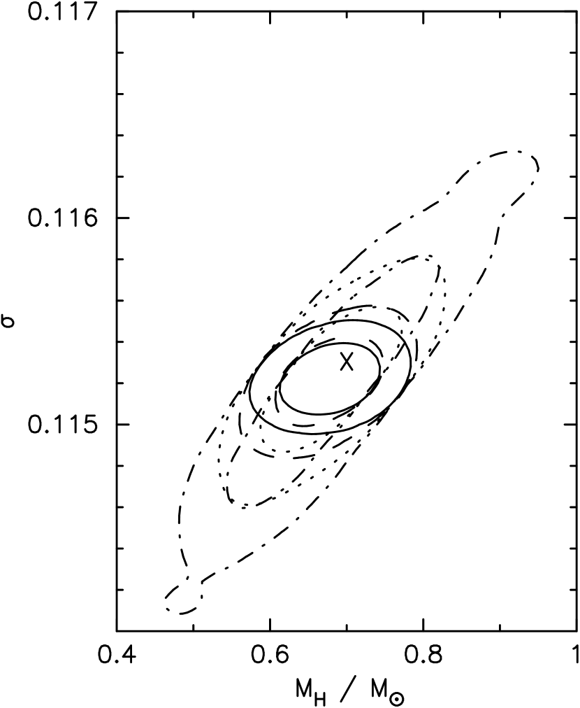
Figure 7: Contours containing 68 $\%$ and 95 $\%$ of the $N=100$ (dot-dashed line), $316$ (dotted), $1000$ (dashed) and $3162$ (solid) event best fit PBH MFs for the MACHO 2-year (left panel) and perfect flat (right panel) efficiencies.

Figure 8: Contours containing 68 $\%$ and 95 $\%$ of the $N=100$ (dot-dashed line), $316$ (dotted), $1000$ (dashed) and $3162$ (solid) event best fit DF MFs for the MACHO 2 year (left panel) and perfect flat (right panel) efficiencies.

Figure 9: Contours containing 68 $\%$ and 95 $\%$ of the $N=100$ (dot-dashed line), $316$ (dotted), $1000$ (dashed) and $3162$ (solid) event of the halo fraction and mean MACHO mass for the best fit PBH MFs for the MACHO 2 year (left panel) and perfect flat (right panel) efficiencies.

Table 1: The estimated duration, taking into account blending, of the 8 microlensing events from Alcock et. al (1997a).

Event	$\hat{t}$ (days)
1	38.8
2	52
3	88
4	100
5	131
6	70
7	143
8	47

Table 2: Relative maximum likelihood of each mass function/halo model combination, for the 6 event sub–sample.

Mass function	SH	SHVT	B	C
DF	1	0.97	0.99	0.98
PLF	$\rightarrow 1$	$\rightarrow 0.97$	$\rightarrow 0.99$	1.02
PLV	$\rightarrow 1$	$\rightarrow 0.97$	$\rightarrow 0.99$	1.12
SPL	1	0.97	1.00	1.15
PBH	0.92	0.96	0.92	1.10

Table 3: Relative maximum likelihood of each mass function model, for all 8 events and a standard halo.

Mass function	SH8
DF	1.00
PLF	1.03
PLV	1.03
SPL	1.04
PBH	1.00

Table 4: Parameters of best fit delta-function mass functions.

Halo model	$M_{\rm df}/M_{\odot}$	f
SH	0.44	0.50
SHVT	0.50	0.50
B	0.53	0.30
C	0.22	0.041
SH8	0.44	0.68

Table 5: Parameters, and halo fraction and mean MACHO mass, of best fit power law mass function, with fixed upper cut off $M_{{\rm max}}=12M_{\odot}$.

Halo model	$M_{{\rm min}}/M_{\odot}$	$\alpha$	$A_{{\rm n}}$	f	$\bar{M}/M_{\odot}$
SH	$\rightarrow 0.44$	$\rightarrow-\infty$	n/a	0.50	0.44
SHVT	$\rightarrow 0.50$	$\rightarrow-\infty$	n/a	0.50	0.50
B	$\rightarrow 0.53$	$\rightarrow-\infty$	n/a	0.31	0.53
C	0.15	-3.2	2.7 $\times 10^{70}$	0.042	0.27
SH8	0.34	-3.9	$3.0\times 10^{95}$	0.68	0.50

Table 6: Parameters, and halo fraction and mean MACHO mass, of best fit power law mass function, with free upper cut off.

Halo model	$M_{{\rm min}}/M_{\odot}$	$M_{{\rm max}}/M_{\odot}$	$\alpha$	$A_{{\rm n}}$	f	$\bar{M}/M_{\odot}$
SH	$\rightarrow 0.44$	$\rightarrow 0.44$	$\rightarrow-\infty$	n/a	0.50	0.44
SHVT	$\rightarrow 0.50$	$\rightarrow 0.50$	$\rightarrow-\infty$	n/a	0.51	0.50
B	$\rightarrow 0.53$	$\rightarrow 0.53$	$\rightarrow+\infty$	n/a	0.30	0.53
C	0.08	0.44	0.2	$1.7\times 10^{-41}$	0.041	0.27
SH8	0.25	0.66	0.5	$2.75\times 10^{-50}$	0.67	0.47

Table 7: Parameters, and halo fraction and mean MACHO mass, of best fit symmetric power law mass function.

Halo model	$M_{{\rm c}}/M_{\odot}$	$M_{{\Delta}}/M_{\odot}$	$\alpha$	$A_{{\rm n}}$	f	$\bar{M}/M_{\odot}$
SH	0.44	0.04	0.4	$4.5\times 10^{-33}$	0.50	0.44
SHVT	0.50	0.04	0.4	$4.2\times 10^{-38}$	0.50	0.50
B	0.53	$\rightarrow 0$	$\rightarrow 0$	n/a	0.30	0.52
C	0.27	0.20	3.1	$5.9\times 10^{-35}$	0.042	0.27
SH8	0.30	0.52	8.4	$5.9\times 10^{-34}$	0.69	0.52

Table 8: Parameters, and halo fraction and mean MACHO mass, of best fit PBH mass functions.

Halo model	$M_{{\rm H}}/M_{\odot}$	$\sigma(M_{{\rm H}})$	$f$	$\bar{M}/M_{\odot}$
SH	0.70	0.1153	0.51	0.50
SHVT	0.80	0.1155	0.51	0.57
B	0.87	0.1141	0.32	0.61
C	0.38	0.1071	0.042	0.26
SH8	0.73	0.1164	0.70	0.52

Table 9: Mean and standard deviation (SD) of best fit values of $M_{{\rm H}}$ and $\sigma$ obtained from Monte Carlo simulations, using the 2 year MACHO collaboration efficiency.

$N_{{\rm e}}$	$\bar{M}_{{\rm H}}/M_{\odot}$	SD ($M_{{\rm H}}/\bar{M_{\rm H}})$	$\bar{\sigma}$	SD ($\sigma/\bar{\sigma}$)
100	0.681	0.125	0.11519	$3.6\times 10^{-3}$
316	0.676	0.068	0.11518	$1.9\times 10^{-3}$
1000	0.674	0.038	0.11517	$1.0\times 10^{-3}$
3162	0.677	0.024	0.11518	$6.9\times 10^{-4}$

Table 10: Mean and standard deviation (SD) of best fit values of $M_{{\rm H}}$ and $\sigma$ obtained from Monte Carlo simulations using the perfect flat efficiency.

$N_{{\rm e}}$	$\bar{M}_{{\rm H}}/M_{\odot}$	SD ($M_{{\rm H}}/\bar{M}_{\rm H}$)	$\bar{\sigma}$	SD ($\sigma/\bar{\sigma}$)
100	0.714	0.125	0.11534	$3.6\times 10^{-3}$
316	0.704	0.065	0.11530	$1.8\times 10^{-3}$
1000	0.708	0.041	0.11533	$1.1\times 10^{-3}$
3162	0.708	0.024	0.11533	$6.9\times 10^{-5}$

References

- (1) Afonso C. 1998, A&A, 337 L17
- (2) Alcock C. et. al. 1995, ApJ, 449, 28
- (3) Alcock C. et. al. 1996a, Nucl. Phys. Proc. Suppl. 51B, 152
- (4) Alcock C. et. al. 1996b, ApJ, 461, 84
- (5) Alcock C. et. al. 1997a, ApJ, 486, 697
- (6) Alcock C. et. al. 1997b, ApJ, 491L, 11
- (7) Alcock C. et. al. 1999, ApJ, 518, 44
- (8) Alcock C. et. al. 2000, preprint astro-ph/0001272
- (9) Ansari R. et. al. 1997, A&A, 324, 843
- (10) Ashman K. M. 1992, PASP, 104, 1109
- (11) Aubourg E. Palanque-Delabrouille, N. Salati, P. Spiro, M. & Taillet R., 1999, A&A, 347, 850
- (12) Bennett D. 1998, Phys. Rept. 307, 97
- (13) Boden A. , Shao M., & van Buren D. 1998, ApJ, 502 538
- (14) Carr B. J. , & Hawking S. W. 1974, MNRAS 168, 399
- (15) Carr B. J. 1975, ApJ, 201, 1
- (16) Carr B. J. 1994, ARAA, 32, 531
- (17) Carr . B. J. 1996, in Current Topics in Astro-fundamental Physics, Proceedings of the Internat. School of Astrophysics ‘D. Chalonge’, edited by N. Sanchez and A. Zichichi (World Scientific Singapore).
- (18) Charlot S. & Silk J. 1995, ApJ, 445, 124
- (19) Crawford M., & Schramm D. N. 1982, Nature, 298, 538
- (20) Evans N. W. 1993, MNRAS, 260, 191
- (21) Evans N. W. 1994, MNRAS, 267, 333
- (22) Evans N. W., Gyuk G., Turner M. S., & Binney J. 1998, ApJ, 501L, 45
- (23) Evans N. W., & Kerins E. J. 1999, astro-ph/9909254
- (24) Flynn C., Sommer-Larsen J., Fuchs B., Graff D. S., & Salim S., 1999, preprint, astro-ph/9912264
- (25) Freeman K. C. 1995 in IAU Symp. 169, Unsolved problems of the Milky Way ed. L. Blitz (Dordrecht: Kluwer)
- (26) Freese K., Fields B., & Graff D. 1999, astro-ph/9901178 to appear in the proceedings of the International Workshop on Aspects of Dark Matter in Astro and Particle Physics, Heidelberg, Germany, July 1998.
- (27) García-Bellido J., Linde A., & Wands D. 1996, Phys. Rev. D 54, 6040
- (28) Gould A., & Salim A. 1999, ApJ 524, 794
- (29) Graff D. S., Gould A., Suntzeff N., Schommer B., & Hardy B. 1999, preprint astro-ph/9910360
- (30) Green A. M., & Liddle A. R. 1997, Phys. Rev. D 54, 6166
- (31) Green A. M., & Liddle A. R. 1999, Phys. Rev. D 60, 063509
- (32) Griest K., 1991, ApJ, 336, 412
- (33) Gyuk G., & Crotts A. 1999, preprint, astro-ph/9904314
- (34) Gyuk G., Dalal N., & Griest K. 1999, preprint, astro-ph/9907338
- (35) Gyuk G., & Gates E. 1999, MNRAS, 304, 281
- (36) Hansen B. M. S. 1999a, ApJ, 517, L39
- (37) Hansen B. M. S. 1999b, ApJ, 520, 680
- (38) Harrison E. R. 1970, Phys. Rev. D 1, 2726
- (39) Helmi A., White S. D. M., de Zeeuw P. T., & Zhao H. 1999, Nature, 402, 53
- (40) Honma M. 1999, ApJ, 511, L100
- (41) Ibata R. A., Richer H. B., Gilliland R. L., & Douglas S. 1999, ApJ, 524, L95
- (42) Ioka K., Chiba T., Tanaka T., & Nakamura T. 1998, Phys. Rev. D 58, 063003
- (43) Ioka K., Tanaka T., & Nakamura T. 1999, Phys. Rev. D 60 083512
- (44) Ivanov P., Naselsky P., & Novikov I. 1994, Phys. Rev. D. 50, 7173
- (45) Jedamzik K. 1997, Phys. Rev. D 55, R5871
- (46) Jedamzik K., & Niemeyer J. C. 1999 Phys. Rev. D 59, 124014
- (47) Jetzer Ph. 1994, ApJ, 432, L43
- (48) Johnson R. A., Gilmore G. F., Tanvir N. R., & Elson R. A. W. 1999, NewA 4, 431
- (49) Jones B. F., Klemola A. R., & Lin D. N. C. 1994, AJ, 107, 133
- (50) Kerins E. J., & Evans N. W. 1999, ApJ, 517, 734
- (51) Kochanek C. S. 1995, ApJ, 445, 559
- (52) Liddle A. R., & Lyth, D. H. 1993, Phys. Rep. 231, 1
- (53) Mao S., & Paczńyski B. 1996, ApJ, 473, 57
- (54) Markovic D. 1998 MNRAS, 507, 316
- (55) Markovic D., & Sommer-Larsen J. 1997, MNRAS, 229, 929
- (56) Moore B. et. al. 1999, ApJ, 524, L19
- (57) Nakamura T. Sasaki M. Tanaka T., & Thorne K. 1997, ApJ, 487, L139
- (58) Niemeyer J. C., & Jedamzik K. 1998, Phys. Rev. Lett. 80, 5481
- (59) Niemeyer J. C., & Jedamzik K. 1999, Phys. Rev. D 59, 124013
- (60) Paczyński B. 1986, ApJ, 428 L5
- (61) Palanque-Delabrouille N. et. al. 1997, A&A, 332, 1
- (62) De Paolis, F., Ingrosso G., & Jetzer Ph. 1996, ApJ, 470, 493
- (63) Primack J. R., Sadoulet, B., & Seckel D. 1988, Ann. Rev. Nucl. Part. Sci., B38, 751
- (64) Randall L., Soljac̆ić M., & Guth, A. H. 1996 Nucl. Phys. B. 472, 377
- (65) De Rujula A., Jetzer, Ph., & Masso E. 1991, MNRAS, 250, 348
- (66) Sackett P. D. et. al., 1994, ApJ, 436, 629
- (67) Sahu K. C., & Sahu M. S. 1999, ApJ, 508L, 147
- (68) Salati P., Taillet R. Auborg E., Palanque-Delabrouille N., & Spiro M. 1999, A&A, 350 L57
- (69) Schmid C., Schwarz D. J., & Widerin P. 1999, Phys. Rev. D 59, 043517
- (70) Schwarz D., J., Schmid C., & Widerin P. 1997, Phys. Rev. Lett. 78, 791
- (71) Stubbs C. W., 1998 astro-ph/9810488, invited talk at Third Stromlo Symposium
- (72) Widrow L. M., & Dubinski J. 1998, ApJ, 504, 12
- (73) Yokoyama J. 1995, astro-ph/9509027
- (74) Zaritsky D., & Lin D. N. C. 1997, AJ, 114, 2545
- (75) Zaritsky D., Shechtman S. A., Thompson I., Harris J., & Lin D. N. C. 1999, AJ, 117, 2268
- (76) Zhao H. 1998, MNRAS, 294, 139
- (77) Zhao H. 1999, astro-ph/9902179, to appear in Particle Physics and the Early Universe, AIP Proc. ed. David Caldwell