The Optical Depth to Reionization as a Probe of Cosmological and Astrophysical Parameters

Abstract

Current data of high-redshift absorption-line systems imply that hydrogen reionization occurred before redshifts of about 5. Previous works on reionization by the first stars or quasars have shown that such scenarios are described by a large number of cosmological and astrophysical parameters. Here, we adopt a semi-analytic model of stellar reionization in order to quantify how the optical depth to reionization depends on such parameters, and combine this with constraints from the cosmic microwave background (CMB). We find this approach to be particularly useful in alleviating the well-known degeneracy in CMB parameter extraction between the optical depth to reionization and the amplitude of the primordial power spectrum, due to the complementary information from the reionization model. We also examine translating independent limits on astrophysical parameters into those on cosmological parameters, or conversely, how improved determinations of cosmological parameters will constrain astrophysical unknowns.

1 Introduction

Observations of the spectra of distant quasars and galaxies have revealed the absence of a Gunn-Peterson trough, implying that the intergalactic medium (IGM) was highly ionized by redshifts of about 5. Since the universe recombined at redshifts, $z$ $\sim$ 1100, the IGM is expected to remain neutral until it is reionized through the activity of the first luminous sources. At present, it appears that the reionization of hydrogen occurred before $z\sim 5$ (Schneider et al., 1991; Hu et al., 1999; Spinrad et al., 1998), while that of doubly ionized helium is thought to have occurred before $z\sim 3$ (Hogan et al., 1997; Reimers et al., 1997).

The ionizing sources responsible for reionization can be a variety of astrophysical objects, and much work has been done on reionization by the first stars (Haiman & Loeb, 1997; Fukugita & Kawasaki, 1994), the first quasars (Haiman & Loeb, 1998a; Valageas & Silk, 1999), proto-galaxies (Cen & Ostriker, 1993; Gnedin, 2000; Giroux & Shapiro, 1996; Ciardi et al., 2000; Miralda-Escude et al., 2000; Madau et al., 1999), and related phenomena such as supernova-driven winds (Tegmark et al., 1993), and cosmic rays (Nath & Biermann, 1993). Quasars are natural candidates for both H I and He II reionization, as they are more luminous and provide harder ionizing radiation relative to stars, and they are seen up to the highest redshifts of current observations. However, there are indications of a turnover in the space density of the QSO population, which apparently decreases beyond $z\sim 3$. As this is based on optical surveys, this observed decline is subject to the effects of any dust obscuration along the line of sight; however, recent radio observations also appear to indicate a declining QSO population beyond $z\sim 3$, so that the comoving emission rate of Lyman continuum photons from QSOs is deficient by a factor of $\sim$ 4 relative to that required for reionization (see, e.g., Madau (1998) and references therein). If this is real, then QSOs may be less plausible as sources for H I reionization (see also Rauch et al. (1997)). The alternative is to allow QSO formation in collapsing halos from the outset, and to postulate a large population of faint QSOs at $z\gtrsim 5$, with the observed turnover being true for bright QSOs only.

Stellar reionization is attractive for several reasons. The first stars are expected to form at $z\gtrsim 10$, and are capable of ionizing hydrogen. Furthermore, they create heavy elements, and may account for the low (0.01 $Z_{\odot}$) but persistent metallicity seen in the Ly-$\alpha$ forest clouds out to $z\sim 4$. Finally, the detections of a He II absorption trough in high-$z$ quasar spectra appear to indicate a soft component to the UV background (Haardt & Madau, 1996), consistent with the ionizing spectrum of stars.

Early work on hydrogen reionization (Arons & Wingert, 1972) described the appearance of the first luminous sources, about which ionized bubbles gradually expand into a neutral IGM; eventually such H II regions overlap and the universe becomes transparent to Lyman continuum photons. In principle, only one ionizing photon per neutral atom in the IGM is required, but the effects of recombinations ensure that for an atom to stay ionized, the rate of ionizing photons generated by sources must be greater than the rate of recombination at that epoch. This is of particular importance at high $z$’s, when the IGM had greater density. Just how much more than 1 photon per baryon is needed is a function of the cosmology and the assumptions of the reionization treatment; some evolution with redshift is also expected. A qualitative assessment may be made however; for example, from arguments of producing the average IGM metallicity in C IV of about 10${}^{-2}Z_{\odot}$ at $z\lesssim 5$, Miralda-Escude & Rees (1997) arrived at a requirement of 20 ionizing photons per baryon. For the stellar reionization model that will be considered in this work, we will see below that about 5 ionizing photons per baryon are available for H I reionization and prove sufficient. Not more than a few percent of all baryons need participate in early star formation for reionization to occur by $z\sim 5$, though this number may reach values of up to about 15% (§2).

Though reionization by early stars would occur at redshifts well beyond current observations, it has many distinct consequences which can be feasibly constrained by current and future experiments. Some of these include, as mentioned above, the evolving IGM metallicity and the cosmic ionizing background as derived from spectral features in high-$z$ absorption-line systems. High-$z$ reionization will also leave a signature in the CMB through the Thomson scattering of CMB photons from free electrons (Sugiyama et al., 1993; Dodelson & Jubas, 1995; Tegmark et al., 1994; Tegmark & Silk, 1995; Hu, 2000; Zaldarriaga, 1997). Depending on the epoch and degree of reionization, we expect an overall (somewhat scale-dependent) damping of primary temperature anisotropies in the CMB, the generation of new temperature anisotropies on the appropriate scales through the effects of second-order processes and the degree of inhomogeneity in the reionization process (Gruzinov & Hu, 1998; Knox et al., 1998), and finally, the creation of a new polarization signal, as the process of Thomson scattering introduces some degree of polarization even for incident radiation that is unpolarized. Scattering from the ionized IGM, or the reprocessing of starlight into far-infrared wavelengths by dust formed from early supernovae (SNe), will also cause the CMB to undergo some spectral distortion (Loeb & Haiman, 1997); this can be measured experimentally through the Compton $y$-parameter. These and other observational signatures that have the potential to constrain the epoch, and hence possibly the source, of reionization have been examined in the literature (see Haiman & Knox (1999) for a summary).

A model of reionization is therefore, in principle, eminently testable. Current detections of the first Doppler peak in the CMB’s temperature anisotropies limit the total optical depth to electron scattering, $\tau_{e}$, such as may arise from reionization, to be $\tau_{e}\lesssim 1$ (Scott et al., 1995). Future experiments such as the Next Generation Space Telescope (NGST) or the Space Infrared Telescope Facility ($SIRTF$) may detect the high-$z$ sites of reionizing sources (see, e.g., Haiman & Loeb (1998b)), or at least exclude currently viable candidates, while upcoming CMB experiments such as $MAP$ or the PLANCK surveyor can measure $\tau_{e}$ to very high accuracies by combining information from temperature anisotropies and polarization in the CMB.

The optimistic prospects for testing reionization and the increasing multiwavelength view of the high-$z$ universe have generated a large body of work on reionization models in the last few years, whose techniques fall broadly into numerical (Gnedin, 2000; Chiu & Ostriker, 2000; Gnedin & Ostriker, 1997; Cen & Ostriker, 1993) or semi-analytic methods (Haiman & Loeb, 1997, 1998a; Tegmark et al., 1994; Valageas & Silk, 1999). The former have the advantage of being able to track the details of radiative transfer, incorporating the clumpiness of the IGM and the essentially non-uniform development of ionizing sources, and, perhaps most importantly, describing the process of reionization in a quantitative fashion. The advantage of semi-analytic approaches is their inherent flexibility and ability to probe the parameter space of a reionization model at will, which is of value given the many input cosmological and astrophysical parameters involved.

For astrophysical sources, the process of reionization is strongly related to the evolution of structure in the universe, and could result in feedback effects for subsequent object formation (see, e.g., Ciardi et al. (2000)). Of the current theories of structure formation, variants of the standard cold dark matter (sCDM) model are considered to be relatively successful at describing the observed universe. This picture postulates a critical density universe, with cold dark matter dominating the matter content; structures, made up of baryons and CDM, originated in primordial adiabatic fluctuations and evolved subsequently through gravitational instability. Current modifications to this paradigm include, e.g., the addition of a cosmological constant.

The sCDM model, and its variants, are described by a set of parameters which characterize the primordial power spectrum of fluctuations, the cosmology of the universe, and quantities related to primordial nucleosynthesis. At present, the extraction of such parameters from observations has been made feasible by the quality of data from large-scale structure surveys, from cosmic velocity flows (Zehavi & Dekel, 1999), from Type Ia SNe (Tegmark, 1999), and from current and projected future data from the CMB (Zaldarriaga et al., 1997; Eisenstein et al., 1999). Typically, a 9–13 parameter set describes the adiabatic CDM model, and can be solved for given the data. One of these parameters is $\tau_{e}$, which is by nature somewhat unique, in that it is the only quantity that is not set purely by the physics prior to the first few minutes after the Big Bang. Thus it can potentially provide clues on post-recombination astrophysics, assuming that the other (cosmological) parameters which also affect $\tau_{e}$ are comparatively well-constrained.

Several of the semi-analytic works on reionization mentioned above have explored the effects of varying model parameters on $\tau_{e}$. Other authors have performed CMB analyses that have revealed inherent degeneracies in constraining specific combinations of parameters, e.g., $\tau_{e}$ and the amplitude of the primordial power spectrum, $A$ (see, e.g., Zaldarriaga et al. (1997); Eisenstein et al. (1999)). In this paper, we examine the results of cross-constraining the range in a cosmological parameter, given the allowed band in $\tau_{e}$ from a reionization model due to astrophysical parameter uncertainty, with the permitted range from CMB observations. Specifically, we find that for the combination $\tau_{e}$–$A$, the well-known degeneracy in their effects on the CMB can be broken when used in combination with the constraints from a reionization model. As $\tau_{e}$ depends on both cosmological and astrophysical parameters, however, such an analysis can be extended to mutual constraints involving these two independent classes of parameters, by eliminating $\tau_{e}$. The advantage of this is that, given a model of structure formation and a reasonable framework describing reionization, as well as the data from the CMB, we can use known astrophysics to further constrain cosmology and place tighter limits on cosmological parameters, even those that will be determined to high accuracies by future experiments. Conversely, a well-determined cosmological parameter can be used to constrain the astrophysics of ill-known details of early star formation. This will, at the least, be a powerful test of the cosmology, if our understanding of reionization is reasonably correct; the additional hope is that this will prove to be an alternative way of constraining the activity of the first stars.

The plan of the paper is as follows. In §2, we outline the stellar reionization scenario that we consider, and set up a parameter set that describes reionization. In §3, we review the standard methodology related to parameter extraction from the CMB, and incorporate the parameter set from §2 into this formalism. In §4, we present our results, and show the combined constraints from a reionization model and the CMB. We present our conclusions in §5.

2 The Stellar Reionization Model

We assume a sCDM primordial power spectrum of density fluctuations, given by $P(k)=Ak^{n}T^{2}(k)$, where $A$ and $n$ are, respectively, the amplitude and index of the power spectrum, and the matter transfer function $T(k)$ is taken to be the form given in Bardeen et al. (1986), with the baryon correction as given by Peacock & Dodds (1994). Here, we evaluate the power spectrum normalization $A$ through the value of the rms density contrast over spheres of radius 8 $h^{-1}$ Mpc today, $\sigma_{8}$. The cosmology of our model is also described by $\Omega_{0}$, the cosmological density parameter, $\Omega_{b}$, the density parameter of baryons, and $h$, the Hubble constant in units of 100 km s^-1 Mpc^-1. We will assume that $\Omega_{0}=1$ throughout this work, and thus will not include it in the parameter set to be varied in what follows. We assume that there are no tensor contributions to $P(k)$, and set the cosmological constant to be zero. Thus, our cosmological parameter set is [$A$, $n$, $\Omega_{b}$, $h$].

The reionization of the universe by the first generations of stars is described by the model developed in Haiman & Loeb (1997) (henceforth HL97), with the minor modifications described below. Briefly, the fraction of baryons in collapsed dark matter halos, $F_{B}$, is followed using the Press-Schechter formulation; of these baryons, a fraction $f_{\star}$ cool and form stars in a Scalo initial mass function (IMF). A fraction $f_{esc}$ of the generated ionizing photons is assumed to escape from the host object and propagate isotropically into the IGM. One can then solve for the size of the ionized regions associated with each such star-forming cloud, which, when integrated over all haloes, yields at each $z$ the average ionization fraction of the universe, given by the filling factor of ionized hydrogen by volume ($F_{HII}$). We assume that the IGM is homogeneous, in which case the ionized region created by each source can be taken to be spheres of radius $r_{i}$. Reionization is defined to occur when $F_{HII}$ = 1. The total optical depth for electron scattering, $\tau_{reion}$, to the reionization redshift $z_{reion}$, is given by integrating the product of the electron density, the ionization fraction, and the Thomson cross section along the line-of-sight from the present to $z_{reion}$. The cosmology of the universe enters $\tau_{reion}$ through the first two terms of the integrand, and also through the path length of the photons last scattered at $z_{reion}$.

Our adopted model is summarized by the following equations for an $\Omega_{0}=1$ universe:

$$F_{B}(z)=\rm{erfc}(\frac{\delta_{c}}{\sqrt{2}\sigma(R,z)})$$ (1)

$$F_{HII}(z)=\rho_{B}(z)\int_{z_{\star}}^{z}dz_{on}\frac{dF_{B}}{dz}(z_{on})\;(\frac{4\pi}{3M}r_{i}^{3}(z_{on},z))$$ (2)

$$\tau_{reion}=0.053\;\Omega_{b}\;h\int_{0}^{z_{reion}}dz\;\sqrt{1+z}\;(1-f_{\star}F_{B}(z))F_{HII}(z)$$ (3)

The critical overdensity $\delta_{c}\equiv 1.686$, $\sigma(R,z)$ is evaluated with a spherical top-hat window function over a scale $R\propto M_{C}$, where $M_{C}$ is the minimum halo mass that collapses at a given redshift. While a natural choice for $M_{C}$ is the baryonic Jeans mass, given by $\sim 10^{6}M_{\odot}[(1+z)/100]^{1.5}$, this assumes that collapsing halos at a given mass scale are equivalent to star-forming halos. However, several authors (Tegmark et al., 1997; Haiman et al., 1996) have argued for a higher value of $M_{C}$, based on the requirement of an effective coolant for baryons in a halo to fragment into stars. The picture is as follows: the very first stars form from metal-free gas and cool through primordial molecular hydrogen. The universe at that epoch is transparent to photons in the energy range 11.2–13.6 eV, but is opaque to more energetic photons. This initial trace level of stellar activity easily photodissociates the remaining H₂ in the universe (whose abundance relative to H I is very low), well before the H I ionizing flux has built to values sufficient for reionization (see HL97 and references therein). Subsequent halo formation continues but star formation halts as there is no coolant available, and can only resume when halos more massive than $10^{8}M_{\odot}[(1+z)/10]^{-1.5}$ collapse, which can utilize line cooling by atomic H. We set $M_{C}$ to be this higher value, with the understanding that $F_{B}$ now represents the fraction of all baryons that are in star-forming halos. Finally, $z_{\star}$ is the earliest redshift at which the first stars can form, and here we set it to be 100. Prior to this, the temperature of the IGM is coupled to that of the CMB, and the CMB photons are still energetic enough to photodestroy H^-, thus preventing the formation of H₂ through the H^- channel, an important cooling mechanism for structures at these high redshifts to fragment into stars.

The evolution of an individual ionization front is characterized by the ionization radius $r_{i}$, and for a time-dependent source luminosity, can be solved for through a differential equation as in HL97, where the rate of emission of ionizing photons from a stellar population of metallicity $Z=10^{-4}Z_{\odot}$ was constant for about 2 million years before declining with the death of the massive stars in the IMF. In this work, we use the analytic solution from Shapiro & Giroux (1987) (SG87 hereafter) for the evolution of $r_{i}$ in an expanding universe in units of the Strömgren radius $r_{s}$. The Strömgren radius represents the equilibrium reached in the IGM between a source’s ionizing photon rate and the IGM’s recombination rate; $r_{s}$ increases with decreasing $z$, or equivalently, with decreasing average IGM density. The maximum value that $r_{i}$ can have is $r_{s}$; only sources at very high redshifts ($\sim 100$) have ionized regions that fill their Strömgren spheres [SG87]. Note that as the SG87 solution does not account for time-varying sources, we expect $\tau_{reion}$ to be overestimated (reionization occurs earlier) compared to HL97, but as we will see in the next section, this is a very slight effect. Thus, in this work, $r_{i}=(r_{i}/r_{s})_{SG87}\,r_{s}$, where $r_{s}^{3}=3S(0)/(4\pi\alpha_{B}n_{H}^{2}(z))$, $\alpha_{B}=2.6\times 10^{-13}$ cm³ s^-1, and the initial emission rate of ionizing photons leaving the host object is $S(0)$. $F_{HII}(z)$ (see eq. [2]) is determined at each redshift $z$ by integrating over the product of the rate of new halos that formed stars at a turn-on redshift $z_{on}$ (where $z<z_{on}<z_{\star}$), and the ionized volume per unit mass associated with such objects, for a source mass $M$. A detailed treatment of the evolution of $F_{B}$ and $F_{HII}$ with $z$, given various choices of input parameters, may be found in HL97. For their standard model, $F_{B}$ rises rapidly from values of $\sim$ 10^-3 at $z\sim 20$ to about 0.1 at $z\sim 10$; during this period, $F_{HII}$ rises steeply from about 10^-4 ($z\sim 32$) to unity at $z\sim 18$, so that reionization occurs relatively quickly with the growth of $F_{B}$.

We now see that $\tau_{reion}$ is a function of several cosmological and astrophysical parameters. The astrophysical parameter set is [$f_{\star},M_{C},S(0)$]. $S(0)$ is itself a function of several variables: the choice of the IMF, the metallicity $Z$ of the progenitor stars, $f_{esc}$, $f_{\star}$, and the halo’s mass. The last two factors account for the fraction of star-forming baryons in each halo, while $f_{esc}$ represents the loss of ionizing photons to the host cloud before reaching the IGM. Let us now consider the first two variables. Though there have been some arguments for the IMF to be biased towards high-mass stars in the early universe (Larson, 1998), the details of the nature of star formation under those conditions are still not well understood. In the absence of a convincing theory of primordial star formation, the most reasonable assumption is to take a present-day IMF and calculate the luminosity expected from metal-poor stars. As reionization is affected primarily by the massive stars in any IMF, an IMF in the past biased towards high-mass stars would still have the same emission spectrum of ionizing photons, while one dominated by low-mass stars is unlikely to reionize the universe by $z\sim 5$. We therefore take S(0) to be as given in HL97 for $Z=10^{-4}Z_{\odot}$ stars from standard stellar evolutionary models; it includes the ionizing radiation from stars only, and is steady at $f_{\star}f_{esc}10^{46}$ photons s${}^{-1}M_{\odot}^{-1}$ for about 2 million years before declining rapidly, which is consistent with the value in, e.g., Ciardi et al. (2000). As a rough estimate, this translates to $\sim$ 5 ionizing photons per baryon in the universe, for $f_{\star}$ = 0.05, $f_{esc}$ = 0.2.

The ionizing photon contribution from SNe is relatively small (HL97), but most of the mass assigned to forming stars is eventually returned to the IGM. Therefore, the second factor on the RHS of equation (3) for $\tau_{reion}$ should have an extra contribution $f_{SN}f_{\star}F_{B}$ to account for the extra baryons that are available for new star formation, where $f_{SN}$ is an IMF-averaged fraction of the progenitor mass that is expelled into the IGM at the end of the star’s life. We expect between $\sim$ 50–95% of the parent star’s mass as ejecta, until a point is reached (for stellar masses ranging from 50–100 $M_{\odot}$) where the entire star collapses into a black hole. For the low values of $f_{\star}$ that will be considered here, the product $f_{\star}f_{SN}$ will be a small correction and may be ignored. Moreover, the mass of the ejecta from a dying star depends sensitively on the stellar metallicity, with low-$Z$ stars having higher remnant masses and less ejected material relative to solar-$Z$ stars (Woosley & Weaver, 1995). Thus, $f_{SN}$ is likely to be highly variable, both spatially and with $z$ due to the evolving metallicity of subsequent generations of stars, and is more appropriately modelled in a simulation rather than in a semi-analytic model. The calculated values of $\tau_{reion}$ here may be taken as a lower limit.

This leaves the astrophysical parameters, $f_{\star},f_{esc}$, and $M_{C}$. We note that in most semi-analytic models, $f_{\star}$ is set by the choice of $M_{C}$, as the stellar $Z$-output, particularly in ¹²C, is combined with the evolution of $F_{B}$ to produce the observationally detected average carbon abundance of 0.01 $Z_{\odot}$ in the Ly-$\alpha$ forest clouds at $z\sim 3$ (Songaila & Cowie, 1996). Thus, $f_{\star}$ and $M_{C}$ are not independent of each other if we choose the above normalization; for the HL97 choice of $M_{C}$, $f_{\star}=0.13$. This is the maximum value that $f_{\star}$ can have from arguments of avoiding IGM over-enrichment; given the approximately order-of-magnitude scatter in the average metal abundance of the Lyman-$\alpha$ clouds, and that one need not require the reionizing stars to solely account for $Z_{IGM}$, $f_{\star}$ may be smaller than $\sim$ 0.15.

As an aside for the interested reader, we note here two drawbacks of normalizing $f_{\star}$ via ¹²C. One is that the massive stars in the IMF ($\gtrsim 10M_{\odot}$) are the ones relevant for reionization, while ¹²C is produced dominantly by the intermediate-mass stars (2–8 $M_{\odot}$). Thus, if the IMF was different in the past, the carbon abundance in the Ly-$\alpha$ forest does not constrain the massive or reionizing stellar activity in early halos. The second point to note is that the pause in star formation caused by the initial dissociation of H₂ led to the choice of $M_{C}$, as in HL97. This minimum halo mass corresponds to objects of virial temperature of $\sim 10^{4}$ K. At this temperature, the host object is immune to photoionization heating (as pointed out in HL97), and so if outflows are desired to expel the generated metals into the IGM (i.e, the Ly-$\alpha$ forest), the mechanical energy of SNe must be invoked. Again, the massive reionizing stars end their lives as Type II SNe an order of magnitude in time before their intermediate-mass carbon-producing compatriots. As all the mechanical input lies with Type II SNe, the question arises of how the carbon, produced significantly later, leaves the host halo to mix with the IGM. Furthermore, Type II SNe occur on much more predictable timescales, i.e. immediately following the progenitor’s death, than do Type Ia SNe (3–10 Gyr), and there is not much more than a wheeze to be had from the deaths of intermediate-mass stars as planetary nebulae.

Having voiced these objections, we point out that while the ¹²C connection as made above between $M_{C}$ and $f_{\star}$ is not ideal, postulating a general relation between these two variables is not ad hoc. The value of $M_{C}$ does intrinsically determine the stellar history, metallicity and luminosity evolution of the universe; the high value of $M_{C}$ in HL97 and other works is physically well-motivated by the necessary step of having an available coolant to aid star formation. We proceed to set $M_{C}$ = $10^{8}M_{\odot}[(1+z)/10]^{-1.5}$ for the semi-analytic treatment here, and now narrow our astrophysical parameter set to [$f_{esc},f_{\star}$].

We end here by addressing some of the issues that are not accounted for in this work. The IGM is assumed to be homogeneous, but clearly some clumpiness will develop in the IGM from the growth of initial density inhomogeneities, and the assumption of the average ionized fraction at a given redshift being equal to the H II filling factor will eventually break down. However, this appears to be a relevant effect only at “late” times ($z\lesssim 10$), when the fraction of baryons in collapsed structures becomes significant (Gnedin & Ostriker, 1997), or for baryon-dominated universes [SG87]. Therefore, we will assume that the clumping factor is unity (homogeneous IGM) for the rest of this work. We have also neglected corrections from doubly ionized helium, which is not problematic as the spectrum of photons produced by stars is softer than that from quasars, and is more relevant for H I rather than He II reionization (see, however, Tumlinson & Shull (2000) on the helium-ionizing spectrum from zero-metallicity stars). We have set $F_{HeII}=F_{HII}$, but this introduces an error of not more than a few percent (Tegmark & Silk, 1995). Finally, we have not included the effects of bias in the normalization of the matter power spectrum, i.e., we assume that light traces the underlying mass distribution.

3 Constraints From The Microwave Background

As discussed in the introduction, signatures from reionization are expected in the CMB; an accurate measurement of $\tau_{reion}$ or the detection of post-recombination features in the CMB anisotropies have the power to constrain the reionization epoch and the nature of the sources through the angular scale $\theta(\propto l^{-1}$) on which they affected the CMB. Here, $l$ is defined from expanding the angular power spectrum of the CMB in terms of its multipole moments $C_{l}$ and Legendre polynomials:

$$C(\theta)\equiv\sum_{l=2}^{\infty}\frac{(2l+1)}{4\pi}C_{l}P_{l}(cos\,\theta)$$ (4)

The effect of $\tau_{reion}$ is to introduce an overall damping of the temperature $C_{l}$s (HL97, and references therein), except at the largest scales. As discussed by, e.g., Zaldarriaga et al. (1997), this is practically indistinguishable from the generally reduced values of $C_{l}$ expected from simply having a lower amplitude, $A$, of the primordial power spectrum; the difference between these two effects at the smallest $l$’s is obscured by cosmic variance. While the amount of the damping due to $\tau_{reion}$ is $l$-dependent and can potentially break this degeneracy, the accuracy to which $\tau_{reion}$ can be estimated from temperature anisotropy maps alone is not sufficient to distinguish between these two different effects (Zaldarriaga, 1997).

When combined with the polarization data from the CMB however, $\tau_{reion}$ can be constrained with far greater precision. Linear polarization is generated by the primary temperature quadrupole anisotropy photons scattering off the free electrons in the reionized IGM, and is a relatively clean probe of the epoch of reionization (Zaldarriaga, 1997). The polarization signal is expected at low levels compared to that from temperature anisotropies, and may prove difficult to measure, especially for low optical depths. Nevertheless, $\tau_{reion}$ can be detected, in principle, by future experiments to within 1-sigma errors of, e.g., 0.69 (0.022) without (with) polarization information for $MAP$, and 0.59 (0.004) correspondingly for $PLANCK$ (Eisenstein et al., 1999).

We wish to combine the constraints on cosmological or astrophysical parameters from a reionization scenario with those from the CMB; in order to do this for the latter, we follow the standard prescription as outlined in, e.g., Jungman et al. (1996) and Knox (1995). We assume Gaussian initial perturbations, and that the multipole moments $C_{l}$ are determined by a “true” set of $N$ theoretical parameters [$P_{N}$]. If we define the likelihood function $\mathcal{L}$ of observing a set of $C_{l}$s, given $P_{N}$, then the behavior of $\mathcal{L}$ near its maximum can be quantified in terms of the Fisher information matrix, whose elements are given by the second derivative of the logarithm of $\mathcal{L}$ with respect to pairs of parameters in $P_{N}$. The Fisher matrix then represents the accuracy with which $P_{N}$ can be estimated from a given data set, here the CMB’s experimentally measured $C_{l}$s. Further assuming that $\mathcal{L}$ has a Gaussian form near its maximum, the Fisher matrix is given by:

$$F_{ij}=\sum_{l=2}^{\infty}\frac{1}{\sigma_{l}^{2}}\;\left[\frac{\partial C_{l}(P_{N})}{\partial P_{i}}\frac{\partial C_{l}(P_{N})}{\partial P_{j}}\right],\;\;1\leq i,j\leq N$$ (5)

where $\sigma_{l}$ is a measure of how the observed $C_{l}$s are distributed about the mean value of the true $C_{l}(P_{N})$s. We assume that $\sigma_{l}$ is cosmic-variance-limited, and ignore terms arising from the instrumental noise associated with an experiment and from any foregrounds. For a sky fraction $f_{\rm sky}$ that has been mapped, $\sigma_{l}$ can be approximated by:

$$\sigma_{l}= \sqrt{\frac{2}{(2l+1)f_{\rm sky}}}\;C_{l}(P_{N}) (l\leq l_{max})$$ (6)

$$\infty (l>l_{max})$$

We will consider two cases here: ($l_{max}$ = 400, $f_{\rm sky}$ = 0.01), which is roughly representative of data from current CMB experiments, and ($l_{max}$ = 3000, $f_{\rm sky}$ = 0.8) for the data expected from $PLANCK$. As we neglect any experimental or systematic effects, the power of the $C_{l}$s to constrain $P_{N}$, as presented here, is the “best possible” case. Note also that the above formulae are valid when only the temperature information from the CMB is used. More general expressions for the case of including polarization data may be found in, e.g., Zaldarriaga et al. (1997).

The derivatives of the $C_{l}$s with respect to $P_{N}$ were computed for each parameter using two-sided derivatives with step sizes being chosen so that the value of this derivative remained stable (see, e.g., Eisenstein et al. (1999), Appendix B.1). The $C_{l}$s themselves for a given parameter set were found using the publicly available CMBFAST (v. 2.4.1). Note that the parameter set describing the reionization model is [$A$, $\Omega_{b}$, $h$, $n$, $f_{esc}$, $f_{\star}$], which yields $\tau_{reion}$, whereas the CMB data can determine the cosmological parameters and $\tau_{reion}$, or equivalently, [$P_{\rm cosmo},\tau_{reion}(P_{\rm cosmo},P_{\rm astro})$]. Therefore, when we specify $\tau$ (e.g, to CMBFAST), the cosmological and the astrophysical parameter sets ($P_{\rm cosmo},P_{\rm astro}$) are no longer independent, but are related through the reionization model, and the $C_{l}$ derivatives become:

$$\frac{\partial C_{l}}{\partial P_{\rm cosmo}}=\;\left.\frac{\partial C_{l}}{\partial P_{\rm cosmo}}\right|_{\tau}\;+\;\;\left.\frac{\partial C_{l}}{\partial\tau}\right|_{P_{\rm cosmo}}\frac{\partial\tau}{\partial P_{\rm cosmo}}$$ (7)

$$\frac{\partial C_{l}}{\partial P_{\rm astro}}=\;\frac{\partial C_{l}}{\partial\tau}\frac{\partial\tau}{\partial P_{\rm astro}}$$ (8)

Once the Fisher matrix $F_{ij}$ has been constructed, it can be inverted to give the covariance matrix $\mathcal{C}$ between the parameters $P_{N}$; $\mathcal{C}_{ii}$ represents the minimum variance in the estimate of $P_{i}$. Any 2 $\times$ 2 submatrix of $\mathcal{C}$ can then be extracted, giving the ellipse equation for the joint confidence region in the 2-parameter subspace of interest,

$${\bf[P-P_{N}]}\bullet(\mathcal{C}_{2\times 2})^{-1}\bullet{\bf[P-P_{N}]}=\Delta,$$ (9)

where $\Delta$ is set throughout this work to be at the 68% confidence level.

4 Results

We present our results here from combining the reionization model (§2) and the constraints from the CMB (§3). This analysis assumes that the density perturbation spectrum at the CMB and structure formation scales is described by the same power law. For the choice of parameters in HL97, where $f_{\star}$ = 0.13 and $f_{esc}$ = $f_{esc}(z)$, we obtain $\tau_{reion}$ = 0.0734, or $z_{reion}\sim 18.4$, which only slightly exceeds the HL97 value of $\tau_{reion}$ = 0.07. Henceforth, we will refer to $\tau_{reion}$ as $\tau$ for convenience, noting that $\tau$ is always evaluated to the reionization epoch in this work. We define our standard model (SM), fixing $\Omega_{0}=1$, as given by $A(\sigma_{8}=0.7$) = 1.55 $\times 10^{6}$, $\Omega_{b}$ = 0.05, $h$ = 0.5, $n$ = 1.0, $f_{esc}$ = 0.2, $f_{\star}$ = 0.05, and $\tau$ = 0.0573, with reionization occurring at $z\sim 15.5$.

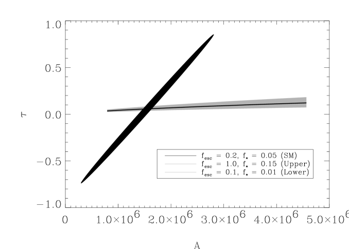
Figure 1: Combined constraints in the $\tau$–$A$ plane from the reionization model and current CMB data. The standard model (SM) is given by the solid line, the shaded band represents the astrophysical uncertainty in the reionization model, given the allowed ranges for ($f_{esc},f_{\star}$), and the ellipse is the 1-$\sigma$ joint confidence region from current CMB data.

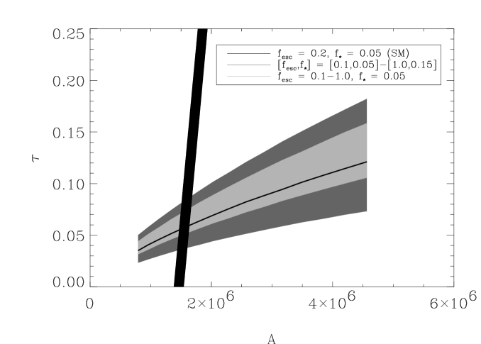
Figure 2: Magnified version of Figure 1; the additional light nested band represents the uncertainty in the value of $f_{esc}$ alone.

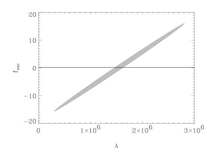
Figure 3: Constraint from current CMB data in the $f_{esc}$–$A$ plane, as extended from Figure 2; the horizontal band is the permitted range of 0.1–0.2 for $f_{esc}$ from DSF.

As a simple example, we begin with the $\tau$–$A$ plane, shown in Figure 1, where we isolate the dependence of $\tau$ on $A$, keeping all the other parameters in the SM fixed. The range of $\sigma_{8}$ is $\sim$ 0.5–0.8, from the large-scale distribution of clusters of galaxies (see, e.g., Bunn & White (1997), and references therein), but is 1.2 when normalized to $COBE$ for the SM choice of cosmological parameters. As an illustrative range for the plots, we normalize $A$ for $\sigma_{8}$ = 0.5–1.2. The solid line represents the SM, while the light shaded region represents the uncertainty due to the astrophysics of the reionization model (or AS for astrophysical slop), with [$f_{esc}$, $f_{\star}$] = [1.0 (0.1), 0.15 (0.01)] for the upper (lower) envelope. The range for $f_{\star}$ (0.01–0.15) is set as follows: the lower limit comes from numerical simulations of star formation (see, e.g., Ciardi et al. (2000), and references therein), while the upper limit corresponds approximately to that in HL97 and Haiman & Loeb (1998a). The value of $f_{esc}$ has been estimated through a number of theoretical and observational methods (see Wood & Loeb (2000), and references therein). Here, we take the range for $f_{esc}$ to be 0.1–1.0, the lower limit coming from Dove et al. (2000) (henceforth DSF), who modelled the escape fraction of ionizing photons from OB stellar associations in the H I disk of the Milky Way, and found that for a coeval star formation history, $f_{esc}$ = 0.15 $\pm 0.05$. Our choice of this limit from DSF is motivated by the similarity of their model’s luminosity history to that in HL97; as noted above, there are alternate values for $f_{esc}$ in the literature for a variety of astrophysical environments. We will use both the full range for $f_{esc}$ and the more narrow DSF band in later plots.

To combine this with the CMB constraint, a shaded ellipse representing the 2-parameter 68% joint confidence region is overplotted, assuming that the true model describing the universe is given by the SM and [$\tau,A$] = [0.057, $A(\sigma_{8}=0.7$)]. This ellipse is narrow enough that we show a magnified version of Figure 1 in Figure 2, with an additional lighter band, nested within the AS band, showing the effect of varying only $f_{esc}$ while fixing $f_{\star}$ to its SM value. We see that the CMB does not really constrain $\tau$ or $A$ separately at all, a near-degeneracy that was expected from the discussion in the previous section. However, the combination of the CMB confidence region and the AS band is much more constraining: this translates to a 1-$\sigma$ error of about 0.02 for $\sigma_{8}$, which is noticeably better than the corresponding value of $\sim$ 0.2 from the CMB ellipse alone.

We now extend Figure 2 to connect, through $\tau$, two a priori independent parameters, $f_{esc}$ and $A$, shown in Figure 3. The purpose of this plot is to probe the potential of cosmology and the astrophysics of reionization to constrain each other, given a reionization model. The ellipse here, as in Figure 1, reveals the inherent degeneracy between $\tau$-related quantities and $A$ through the long narrow ellipse. We now overplot the DSF permitted band for $f_{esc}$ (0.1–0.2); clearly even this approximate range in $f_{esc}$ considerably narrows the allowed range in $A$. We note again that our choice of the DSF range for $f_{esc}$ was motivated for the reasons outlined earlier, and that other ranges for $f_{esc}$ are possible; the main point that is demonstrated by Figure 3 is the power of using any such band of independently known astrophysics to constrain a cosmological parameter. Note also that $A$ would have to be known to great accuracy to place any limits on $f_{esc}$ that are stronger than the DSF band.

Table 1: $V$ AND DIAGONAL ELEMENTS OF $W$ from $F=UWV^{T}$

$\sigma_{8}^{2}$		-0.3922	0.1470	-0.5116	0.7498	-0.0277	0.000
$\Omega_{b}$		-0.5024	-0.8592	0.0916	-0.0320	-0.0028	8.42E-16
$h$		0.5012	-0.3673	-0.7611	-0.1856	-0.0111	3.613E-15
$n$		-0.5840	0.3242	-0.3857	-0.6342	-0.0545	1.599E-14
$f_{esc}$		0.0098	-0.0039	0.0111	0.0041	-0.2539	0.9671
$f_{\star}$		0.0373	-0.0148	0.0420	0.0155	-0.9652	-0.2544
$w$		18110.877	9251.715	330.074	12.455	0.0191	6.366E-16

So far, we have been using the Fisher matrix formalism for specific pairs of parameters, while fixing the values of the other parameters in the SM. The more general and proper way to do this is to construct a 6 $\times$ 6 matrix for the parameter set [$A$, $\Omega_{b}$, $h$, $n$, $f_{esc}$, $f_{\star}$], which yields $\tau$. However, the analysis described in §3 implies that only any five of these six parameters will be independent, as the CMB data will determine the cosmological parameters and $\tau$. Indeed, the 6 $\times$ 6 matrix, when constructed, proves to be singular. We note here briefly some informative aspects of performing singular value decomposition (SVD) (Press et al., 1992) of $F_{6\times 6}$, so that $F$ = $UWV^{T}$, where $W$ is a diagonal $6\times 6$ matrix containing the singular values $w$. An element that has an anomalously low value (close to zero) in $W$ implies that the corresponding column in $V$ is a linear combination of parameters that will not be well-constrained.

Table 1 shows the matrix $V$ with the corresponding column weights $w$ resulting from this decomposition; also shown are the parameters associated with each row in $V$, with $A$ expressed as $\sigma_{8}^{2}$. We see that the sixth weight is very close to zero, so that the sixth column of $V$ contains combinations of [$P_{\rm cosmo},P_{\rm astro}$] that are poorly constrained by this analysis. This column has terms corresponding to essentially only $P_{\rm astro}$, the dominant contribution coming from $f_{esc}$. This implies that $f_{esc}$ will not be well-determined from the CMB (via $\tau$), given the reionization model considered here. The first five columns of $V$ also convey what combinations of these six parameters will be constrained; we note that $f_{esc}$ has very small contributions in these, i.e., to the information that can be extracted from the CMB. In comparison, $f_{\star}$ can be better determined from the CMB, as seen from columns 1–5, particularly the fifth, where the dominant term is from $f_{\star}$. This insensitivity of the CMB data to $f_{esc}$ can be traced back to the stellar reionization model we adopted here; variations in $f_{\star}$ affect $\tau$ more significantly than do those in $f_{esc}$ (see Figures 12 and 15 in HL97).

The covariance matrix for $F$ can be found by, $\mathcal{C}\equiv F^{-1}=VW^{-1}U^{T}$. As the ratio of $W$’s minimum to maximum value, $\sim$ 3 $\times 10^{-20}$, is very small compared with machine precision, we follow the usual technique of adjusting the anomalously low singular value in $W$, here $w_{6}$, to zero (Press et al., 1992); despite this, the SVD inversion of $F$ still produces an inaccurate covariance matrix, i.e., $\mathcal{C}\bullet F\neq I$.

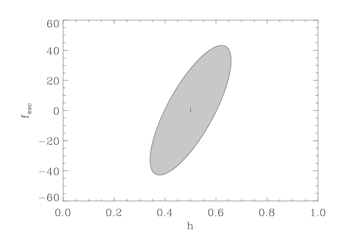
Figure 4: Constraints from the CMB in the $f_{esc}$–$h$ plane; larger ellipse represents current data, and smaller nested ellipse (line) is from $PLANCK$.

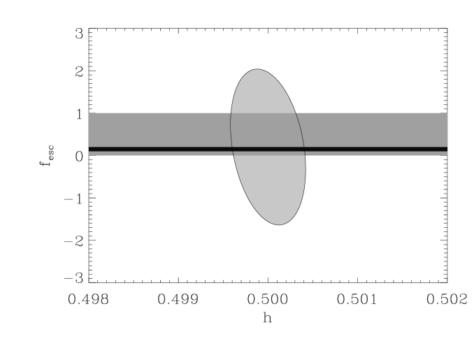
Figure 5: Constraint from $PLANCK$ in the $f_{esc}$–$h$ plane; light shaded band represents the entire allowed astrophysical range of 0.1–1.0 for $f_{esc}$, and the dark shaded band represents the permitted values of 0.1–0.2 for $f_{esc}$ from DSF.

We now proceed to work with the independent 5 $\times$ 5 subportions of the full 6 $\times$ 6 matrix, which translates to $P_{\rm cosmo}$ and any one of $P_{\rm astro}$. These 5 $\times$ 5 matrices are inverted, and the 2 $\times$ 2 submatrix of interest is projected into the 2-parameter plane as the appropriate error ellipse, which displays the confidence region after marginalizing over the other parameters. The results of this general Fisher matrix analysis are presented below for the idealized specifications of current data and for those expected from $PLANCK$ (§3). Only the temperature anisotropies from the CMB are used for Figures 4–11; the polarization information expected from $PLANCK$ is included for Figures 12–13. These plots are intended to be examples of the constraints in various $P_{\rm astro}$–$P_{\rm cosmo}$ subspaces.

Figure 4 shows the case of $f_{esc}$ vs. $h$; the larger ellipse corresponds to current CMB data, and the nested one (appearing as a tiny line) is from $PLANCK$. For all subsequent cases, we show these ellipses separately; the astrophysical range for $f_{esc}$ is omitted from this plot for visual clarity. Figure 5 shows the results expected from $PLANCK$ alone for $f_{esc}$ vs. $h$, with the light shaded horizontal band representing the full range of $f_{esc}$ (0.1–1.0), and the dark band representing the DSF values for $f_{esc}$ (0.1–0.2). The case of $f_{esc}$ vs. $\Omega_{b}$ is shown in Figures 6 and 7, for current CMB data and $PLANCK$ respectively, with the overplotted bands being the same as in Figure 5.

Figures 8–9 and 10–11 display the respective cases of $f_{\star}$ vs. $\sigma_{8}^{2}$ (where $\sigma_{8}^{2}$ $\propto A$), and $f_{\star}$ vs. $n$. For these 4 plots, the horizontal dark band represents the maximum astrophysical range of 0.01–0.15 for $f_{\star}$; values below this range are unlikely to be sufficient for reionization and values above this range must invoke IMFs other than that of present-day galaxies in order to not violate metal production or background light constraints.

We note here some generic features of Figures 5–11. In all cases, the inclusion of known constraints on the astrophysical parameters strengthens the CMB’s limits on cosmological parameters, even for the data expected from $PLANCK$. This is particularly the case with $f_{\star}$, due to $\tau$’s greater sensitivity to $f_{\star}$ relative to $f_{esc}$. Thus the 1-$\sigma$ error for $f_{\star}$ from the CMB is significantly smaller than that for $f_{esc}$ for all the cases shown here, making independent limits on the former a more powerful complementary constraint for cosmological parameters extracted from the CMB. As some illustrative examples involving $PLANCK$ data, the entire astrophysical permitted band for $f_{\star}$ reduces the 1-$\sigma$ error for $\sigma_{8}$ from about 0.02 to less than 0.01 (Figure 9), and for $n$, from 0.006 to $\sim$ 0.004. The power to increase such constraints will only become better as $f_{\star}$ (or $f_{esc}$) become better constrained themselves, but it may not matter much for most cosmological parameters in the post-$PLANCK$ era (as they will already be determined with great precision), with the exception of $A$ or $\sigma_{8}$. For this case, the method here may prove to be a valuable cross-check.

Figures 5–11 also reveal that even the most promising cases of cosmological parameter determination from the CMB’s temperature information will not help to constrain astrophysical parameters such as $f_{\star}$ or $f_{esc}$, whose currently known ranges as shown through the horizontal bands in each figure are typically much smaller than what would be deduced from the joint confidence region. This is partly due to the low value of $\tau$ itself of $\sim$ 0.06 in our SM, which hinders its accurate determination from the CMB data.

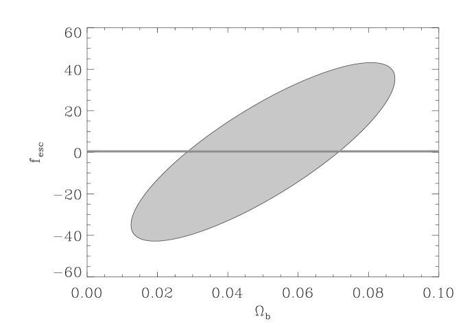
Figure 6: Constraint from current CMB data in the $f_{esc}$–$\Omega_{b}$ plane; shaded bands are the same as in Figure 5.

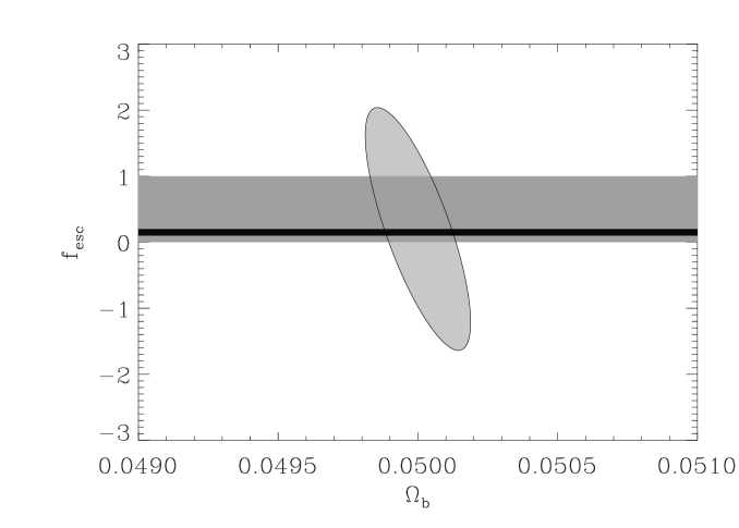
Figure 7: Same as Figure 6, but for data from $PLANCK$.

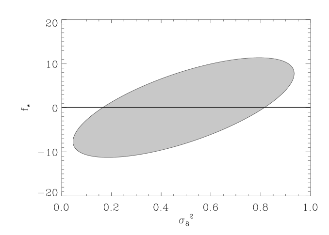
Figure 8: Constraint from current CMB data in the $f_{\star}$–$\sigma_{8}^{2}$ plane, where $\sigma_{8}^{2}\propto A$; shaded band represents the permitted astrophysical range of 0.01–0.15 for $f_{\star}$.

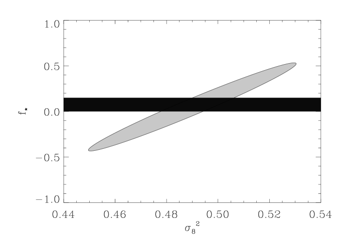
Figure 9: Same as Figure 8, but for data from $PLANCK$.

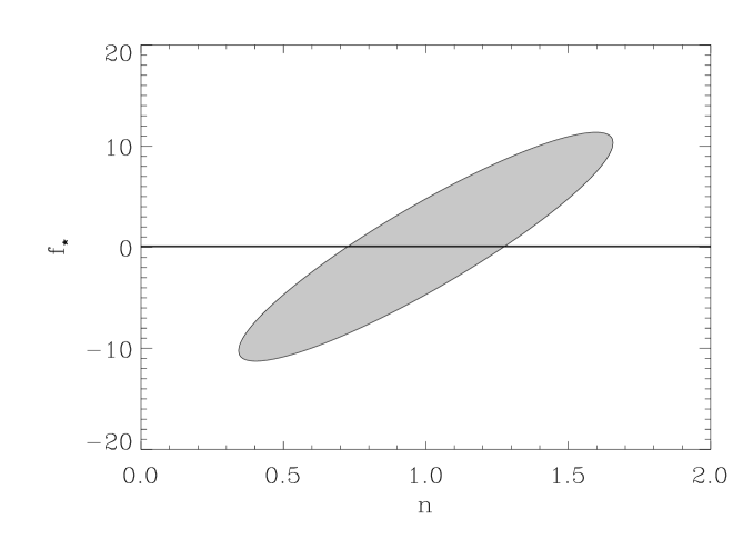
Figure 10: Constraint from current CMB data in the $f_{\star}$–$n$ plane; shaded band is the same as in Figure 8.

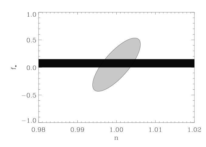
Figure 11: Same as Figure 10, but for data from $PLANCK$.

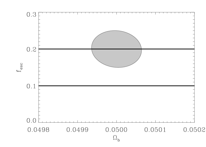
Figure 12: Constraint from $PLANCK$ in the $f_{esc}$–$\Omega_{b}$ plane using temperature and polarization; lines represent the allowed range for $f_{esc}$ from DSF.

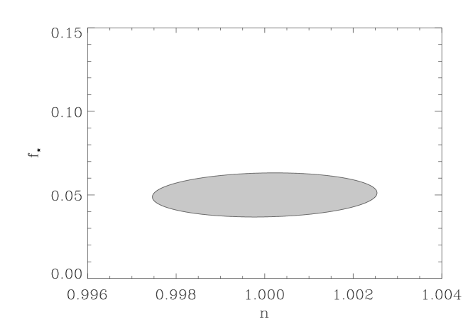
Figure 13: Constraint from $PLANCK$ in the $f_{\star}$–$n$ plane using temperature and polarization; the allowed astrophysical range for $f_{\star}$ is the entire $y$-axis.

When polarization is included for the projected data from $PLANCK$, we see, from the two examples shown in Figures 12–13, that $f_{esc}$ can be determined to about the same accuracy as the DSF allowed band, but that the 1-$\sigma$ error for $f_{\star}$ is significantly smaller than its astrophysical uncertainty. Thus, future CMB data may be able to constrain the astrophysical aspects of reionization. We recall, however, that we have neglected effects from experimental noise or from foregrounds in our analysis, which will enlarge the joint confidence regions in all the figures. While this only strengthens the argument of the power of astrophysical limits in constraining cosmology, the converse situation, which appears hopeful from Figures 12–13, is realistically tentative at best. In short, it is possible in principle that the astrophysics of a stellar reionization model can be constrained by limits on cosmological parameters from $PLANCK$’s temperature and polarization data, though this may prove difficult to achieve. We may simply have to await the view from $SIRTF$ and the $NGST$ to determine the reionizing activity of the first stars!

5 Conclusions

We have examined the power of a reionization model, given its many cosmological and astrophysical parameters, to constrain these input quantities when combined with parameter extraction from the CMB. In the case of the well-known degeneracy between $\tau$ and $A$ in their effects on the CMB, we have found that this can be alleviated by the complementary information from a reionization model, and that this remains a useful cross-constraint even when allowing for the astrophysical uncertainty in $\tau$.

When we eliminate $\tau$ and perform a more general Fisher matrix analysis, we find that the astrophysical details of reionization can be useful in further constraining the CMB’s limits on cosmological parameters, even in the case of the expected temperature data from $PLANCK$. We have shown that independent limits on the astrophysical inputs to reionization, despite the current uncertainty in their values, reduce the errors for cosmological parameters by a factor of at least $\sim$ 2. Given that we have considered the most optimistic parameter yield from CMB experiments (§3), the use of known astrophysics can only become more valuable for realistic experimental results. This is of particular value for $\sigma_{8}$ (or $A$) and $n$, given their implications for structure formation and for theoretical models of the origin of the seeds of structure in the early universe.

The converse situation– using a projected exquisite determination of a cosmological parameter to constrain astrophysical reionization parameters– does not yield quite as interesting results with temperature data from current experiments or from $PLANCK$, even though we made the most optimistic assumptions; the 1-$\sigma$ errors for $f_{esc}$ or $f_{\star}$ are larger than what are already known to be reasonable. When the projected polarization data from $PLANCK$ is included, we found that $f_{\star}$ in particular may be constrained to far greater accuracy than its current astrophysical uncertainty; in practice, however, this may prove difficult to achieve, given the effects of foregrounds and instrumental noise which we have neglected here.

In summary, one may take away that the astrophysical details of reionization can strengthen the limits on the cosmology of our universe, beyond even the projected parameter yield from future CMB data, and that there is more potential to a measurement of $\tau$ than the determination of a single number out of a large parameter space describing adiabatic CDM models. These broad conclusions are naturally subject to the assumptions made in this analysis. The sizes of joint confidence regions derived from the CMB data for any 2-parameter subspace is determined by the full covariance matrix, whose elements’ values are dependent on the dimension of the chosen parameter space and the selected parameters. The inclusion of more parameters has the generic result of increasing the sizes of the error ellipses; therefore, the primary results of this paper can only be strengthened when parameter spaces larger than that analyzed here are considered.

In the sCDM cosmology assumed here, the values of $\tau$ in our standard model were relatively low ($\sim 0.06$). In an open universe, or one dominated by a cosmological constant contribution, we expect larger average values of $\tau$ for a fixed reionization model, as structures freeze out earlier, resulting in a longer line-of-sight to the last scattering surface at the reionization epoch. Increased $\tau$’s can also result from higher values of $f_{\star}$ or $f_{esc}$, or from a lower value of $M_{C}$ (§2), which would allow the first stars to form earlier and more ubiquitously. As higher $\tau$’s will have a better chance of being accurately determined from the CMB, it would be interesting to analyze the constraints in this paper, from both the reionization scenario and the CMB, for a more general parameter space; we examine this in a forthcoming work.

References

- Arons & Wingert (1972) Arons, J. & Wingert, D. W. 1972, ApJ, 177, 1
- Bardeen et al. (1986) Bardeen, J. M., Bond, J. R., Kaiser, N., & Szalay, A. S. 1986, ApJ, 304, 15
- Bunn & White (1997) Bunn, E. F. & White, M. 1997, ApJ, 480, 6
- Cen & Ostriker (1993) Cen, R. & Ostriker, J. P. 1993, ApJ, 417, 404
- Chiu & Ostriker (2000) Chiu, W. A. & Ostriker, J. P. 2000, ApJ, submitted (astro-ph/9907220)
- Ciardi et al. (2000) Ciardi, B., Ferrara, A., Governato, F., & Jenkins, A. 2000, MNRAS, submitted (astro-ph/9907189)
- Dodelson & Jubas (1995) Dodelson, S. & Jubas, J. M. 1995, ApJ, 439, 503
- Dove et al. (2000) Dove, J. M., Shull, J. M., & Ferrara, A. 2000, ApJ, in press, (astro-ph/9903331) [DSF]
- Eisenstein et al. (1999) Eisenstein, D. J., Hu, W., & Tegmark, M. 1999, ApJ, 518, 2
- Fukugita & Kawasaki (1994) Fukugita, M. & Kawasaki, M. 1994, MNRAS, 269, 563
- Giroux & Shapiro (1996) Giroux, M. L. & Shapiro, P. R. 1996, ApJS, 102, 191
- Gnedin (2000) Gnedin, N. Y. 2000, ApJ, in press, (astro-ph/9909383)
- Gnedin & Ostriker (1997) Gnedin, N. Y. & Ostriker, J. P. 1997, ApJ, 486, 581
- Gruzinov & Hu (1998) Gruzinov, A. & Hu, W. 1998, ApJ, 508, 435
- Haardt & Madau (1996) Haardt, F. & Madau, P. 1996, ApJ, 461, 20
- Haiman & Knox (1999) Haiman, Z. & Knox, L. 1999, in ASP Conf. Ser. 181: Microwave Foregrounds, ed. A. de Oliveira-Costa & M. Tegmark, 227, (astro-ph/9902311)
- Haiman & Loeb (1997) Haiman, Z. & Loeb, A. 1997, ApJ, 483, 21, (astro-ph/9611028, v.2) [HL97]
- Haiman & Loeb (1998a) —. 1998a, ApJ, 503, 505
- Haiman & Loeb (1998b) Haiman, Z. & Loeb, A. 1998b, in ASP Conf. Ser. 133: Science With The NGST, ed. E. P. Smith & A. Koratkar, 251, (astro-ph/9705144)
- Haiman et al. (1996) Haiman, Z., Rees, M. J., & Loeb, A. 1996, ApJ, 467, 522
- Hogan et al. (1997) Hogan, C. J., Anderson, S. F., & Rugers, M. H. 1997, AJ, 113, 1495
- Hu et al. (1999) Hu, E. M., McMahon, R. G., & Cowie, L. L. 1999, ApJ, L9
- Hu (2000) Hu, W. 2000, ApJ, submitted (astro-ph/9907103)
- Jungman et al. (1996) Jungman, G., Kamionkowski, M., Kosowsky, A., & Spergel, D. N. 1996, Phys. Rev. D, 54, 1332
- Knox et al. (1998) Knox, L., Scoccimarro, R., & Dodelson, S. 1998, Phys. Rev. Lett., 81, 2004
- Knox (1995) Knox, L. E. 1995, PhD thesis, THE UNIVERSITY OF CHICAGO.
- Larson (1998) Larson, R. B. 1998, MNRAS, 301, 569
- Loeb & Haiman (1997) Loeb, A. & Haiman, Z. 1997, ApJ, 490, 571
- Madau (1998) Madau, P. 1998, in Proceedings of the XVIIIth Moriond meeting “Dwarf Galaxies and Cosmology”, ed. T.X. Thuan, C. Balkowski, V. Cayatte, & J. Tran Thanh Van, (astro-ph/9807200)
- Madau et al. (1999) Madau, P., Haardt, F., & Rees, M. J. 1999, ApJ, 514, 648
- Miralda-Escude et al. (2000) Miralda-Escude, J., Haehnelt, M., & Rees, M. J. 2000, ApJ, in press, (astro-ph/9812306)
- Miralda-Escude & Rees (1997) Miralda-Escude, J. & Rees, M. J. 1997, ApJ, 478, L57
- Nath & Biermann (1993) Nath, B. B. & Biermann, P. L. 1993, MNRAS, 265, 241
- Peacock & Dodds (1994) Peacock, J. A. & Dodds, S. J. 1994, MNRAS, 267, 1020
- Press et al. (1992) Press, W. H., Teukolsky, S. A., Vetterling, W. T., & Flannery, B. P. 1992, Numerical recipes in C. The art of scientific computing (Cambridge: University Press, 2nd ed.)
- Rauch et al. (1997) Rauch, M., Miralda-Escude, J., Sargent, W. L. W., Barlow, T. A., Weinberg, D. H., Hernquist, L., Katz, N., Cen, R., & Ostriker, J. P. 1997, ApJ, 489, 7
- Reimers et al. (1997) Reimers, D., Kohler, S., Wisotzki, L., Groote, D., Rodriguez-Pascual, P., & Wamsteker, W. 1997, A&A, 327, 890
- Schneider et al. (1991) Schneider, D. P., Schmidt, M., & Gunn, J. E. 1991, AJ, 101, 2004
- Scott et al. (1995) Scott, D., Silk, J., & White, M. 1995, Science, 268, 829
- Shapiro & Giroux (1987) Shapiro, P. R. & Giroux, M. L. 1987, ApJ, 321, L107, [SG87]
- Songaila & Cowie (1996) Songaila, A. & Cowie, L. L. 1996, AJ, 112, 335
- Spinrad et al. (1998) Spinrad, H., Stern, D., Bunker, A., Dey, A., Lanzetta, K., Yahil, A., Pascarelle, S., & Fernandez-Soto, A. 1998, AJ, 116, 2617
- Sugiyama et al. (1993) Sugiyama, N., Silk, J., & Vittorio, N. 1993, ApJ, 419, L1
- Tegmark (1999) Tegmark, M. 1999, ApJ, 514, L69
- Tegmark & Silk (1995) Tegmark, M. & Silk, J. 1995, ApJ, 441, 458
- Tegmark et al. (1994) Tegmark, M., Silk, J., & Blanchard, A. 1994, ApJ, 420, 484
- Tegmark et al. (1993) Tegmark, M., Silk, J., & Evrard, A. 1993, ApJ, 417, 54
- Tegmark et al. (1997) Tegmark, M., Silk, J., Rees, M. J., Blanchard, A., Abel, T., & Palla, F. 1997, ApJ, 474, 1
- Tumlinson & Shull (2000) Tumlinson, J. & Shull, J. M. 2000, ApJ, 528, L65
- Valageas & Silk (1999) Valageas, P. & Silk, J. 1999, A&A, 347, 1
- Wood & Loeb (2000) Wood, K. & Loeb, A. 2000, ApJ, submitted (astro-ph/9911316)
- Woosley & Weaver (1995) Woosley, S. E. & Weaver, T. A. 1995, ApJS, 101, 181
- Zaldarriaga (1997) Zaldarriaga, M. 1997, Phys. Rev. D, 55, 1822
- Zaldarriaga et al. (1997) Zaldarriaga, M., Spergel, D. N., & Seljak, U. 1997, ApJ, 488, 1
- Zehavi & Dekel (1999) Zehavi, I. & Dekel, D. 1999, in Proceedings of the Cosmic Flows Workshop, ed. S. Courteau, M. Strauss & J. Willick, (astro-ph/9909487)