Pulsars ellipticity revised

Abstract

We derive new upper limits on the ellipticity of pulsars whose braking index has been measured, more tightening than those usually given, assuming that both a gravitational torque and an electromagnetic one act on them. We show that the measured braking indexes of pulsars are recovered in this model. We consider the electromagnetic torque both constant and varying with time. At the same time constraints on the pulsars initial period and on the amplitude of the gravitational waves emitted are obtained.

1 Introduction

From the timing measurements we deduce that radio pulsars are subject to a systematic secular spin-down. The standard formula for pulsar spin-down is

$$\dot{\Omega}=K\Omega^{n}$$ (1)

The quantity $I\dot{\Omega}$, being $I$ the star momentum of inertia with respect to its rotation axis, is the torque acting on the star and we will refer to $K$, following Allen $\&$ Horvath (horv2 (1997)), as the “torque function”. $K$ and the braking index $n$ depend on the mechanism which is at work. For instance, $n=3$ for pure magnetic dipole radiation and $n=5$ for gravitational radiation. The braking index can be calculated, at least in principle, from the relation

$$n={{\Omega\leavevmode\nobreak\ \ddot{\Omega}}\over{{\dot{\Omega}}^{2}}}$$ (2)

which can be very easily derived from Eq.(1). In practice, only for four pulsars the measure of the braking index is not dominated by the timing noise (Lyne et al. lyne1 (1993)), (Boyd et al. boyd (1995)),(Kaspi et al. kaspi (1994)), (Lyne et al. lyne2 (1996)):

$$Crab:\leavevmode\nobreak\ \leavevmode\nobreak\ \leavevmode\nobreak\ \leavevmode\nobreak\ \leavevmode\nobreak\ n=2.51\pm 0.01$$

$$PSR\leavevmode\nobreak\ 0540-69:\leavevmode\nobreak\ \leavevmode\nobreak\ \leavevmode\nobreak\ n=2.28\pm 0.02$$

$$PSR\leavevmode\nobreak\ 1509-58:\leavevmode\nobreak\ \leavevmode\nobreak\ \leavevmode\nobreak\ n=2.837\pm 0.001$$

$$Vela:\leavevmode\nobreak\ \leavevmode\nobreak\ \leavevmode\nobreak\ \leavevmode\nobreak\ \leavevmode\nobreak\ n=1.4\pm 0.2$$

All these values are less than the canonical value, $3$, which we expect for the emission of dipolar electromagnetic radiation. As we will see in the next section, different mechanisms have been proposed to explain this discrepancy. On the other hand, when pulsars are considered as possible sources of gravitational radiation, the upper limit on the amplitude of the waves emitted is calculated assuming that all the spin-down is due to the emission of gravitational waves, e.g. (Haensel haens (1995)), (Giazzotto et al. giazo (1997)). This implies, see Eq.(14), a braking index equal to 5. Clearly, this is not true, at least for the pulsars whose braking index has been measured. A much more realistic hypothesis is that in a pulsar both an electromagnetic and a gravitational torques work to produce the observed spin-down. We will show how from this assumption the observed braking indexes can be derived and, at the same time, how new more tightening upper limits on the pulsars ellipticity are obtained.

The plan of the paper is the following. In Sec.2 we give the main relations relative to the electromagnetic braking and shortly describe different proposed mechanisms which could produce the observed braking indexes. In Sec.3, after the introduction of the relations describing the gravitational torque, we show how the observed braking indexes can be obtained combining the electromagnetic and gravitational torques. In Sec.4 we calculate, in the framework of our model, the time evolution of various observable quantities, in particular the braking index $n(t)$ and the angular velocity of the pulsar $\Omega(t)$, and derive new upper limits on the ellipticity of pulsars and then, Sec.(5), on the amplitude of the gravitational signals emitted. Finally, in Sec.6 conclusions are discussed.

2 The electromagnetic torque

As it is well known, the electromagnetic torque implies an evolution of the pulsar rotation frequency given by the relation

$$\dot{\Omega}_{em}=K_{em}\Omega^{n_{em}}$$ (3)

The electromagnetic index is $n_{em}=3$ for pure dipolar magnetic radiation (Ostriker $\&$ Gunn ostri (1969)), (Manchester $\&$ Taylor manch (1977)), in which case

$$K_{em}=-{2\over{3c^{3}}}{B^{2}\over{I}}R^{6}\sin^{2}{(\alpha)}$$ (4)

In this equation $B$ is the strength of the magnetic field, $R$ is the neutron star radius, $\alpha$ is the angle between the rotation and the magnetic axes, and $I$ is the momentum of inertia with respect to the rotation axis. An electromagnetic braking index different from 3 can be the consequence of pulsar winds, in which particles having angular momentum are accelerated away from the pulsar (Goldreich $\&$ Julian gold (1969)), (Kaspi et al. kaspi (1994)) or can be produced if non dipolar components of the magnetic field are present, as a consequence of strong magnetospheric currents (Blandford $\&$ Romani roma (1988)). Another possibility is that the magnetic moment, and then the torque applied to the star, varies in time (Blandford $\&$ Romani roma (1988)), (Cheng chen (1989)). Muslimov $\&$ Page (musli (1996)) consider the time evolution of the surface magnetic field of the star, which, according to their model, is very low ($10^{8}\div 10^{9}\leavevmode\nobreak\ G$) for a newborn neutron star and then increases due to the ohmic diffusion of the initially trapped inner magnetic field. The resulting electromagnetic braking index is given by

$$n_{em}=3+2\left({\dot{B}_{surf}\over{B_{surf}}}\right)\left({\Omega\over{\dot{\Omega}}}\right)$$ (5)

where $B_{surf}$ is the value of the surface magnetic field at the magnetic pole. Clearly, if $\dot{B}_{surf}>0$, $n_{em}<3$. Other models based on the secular variation of the magnetic field have been developed, for instance, by Blandford et al. (bland (1983)) and by Camilo (cami (1996)). A different kind of models has been proposed by Allen $\&$ Horvath (horv1 (1997)) and by Link $\&$ Epstein (link (1997)), based on the growth of the angle $\alpha$ between the magnetic moment and the rotation axis of the star. In this case the electromagnetic braking index is

$$n_{em}=3+2{\dot{\alpha}\over{\tan{\alpha}}}\left({\Omega\over{\dot{\Omega}}}\right)$$ (6)

In all these cases the general expression for the observed electromagnetic braking index is simply

$$n_{em}=3+{\dot{K}_{em}\over{K_{em}}}\times{{\Omega}\over{\dot{\Omega}_{em}}}$$ (7)

which is easily obtained deriving Eq.(3) with respect to time. From Eq.(4) we find

$${\dot{K}_{em}\over{K_{em}}}={1\over{B\sin^{2}{\alpha}}}\left[2\dot{B}\sin^{2}{\alpha}+B\sin{2\alpha}\leavevmode\nobreak\ \dot{\alpha}-B\sin^{2}{\alpha}{\dot{I}\over{I}}\right]$$ (8)

Assuming $n_{em}=const$, from Eq.(7) we find

$$K_{em}=K_{em,0}\times\left({\Omega\over{\Omega_{0}}}\right)^{n_{em}-3}$$ (9)

where $K_{em,0}$ and $\Omega_{0}$ are the electromagnetic torque function and the angular velocity at time $t=0$, i.e. now. Then, the rate of variation of the angular velocity can be written as

$$\dot{\Omega}_{em}=K_{em,eff}\Omega^{n_{em}}$$ (10)

where $K_{em,eff}={K_{em,0}\over{\Omega^{n_{em}-3}_{0}}}$ is a constant, which is formally equivalent to Eq.(3). Integrating Eq.(3) we obtain the pulsar “characteristic” time, due to the electromagnetic braking which is:

$$\tau_{em}={\Omega_{0}\over{(1-n_{em})\dot{\Omega}_{0}}}\left[1-\left({\Omega_{0}\over{\Omega_{i}}}\right)^{n_{em}-1}\right]$$ (11)

being $\Omega_{i}$ the initial angular velocity of the pulsar. Eq.(11) would give the true age if only the electromagnetic emission was responsible for the pulsar spin-down.

From Eqs.(3,4), the strength of the magnetic field, for $n_{em}=3$, is

$$B\sin{\alpha}\simeq 3.2\cdot 10^{19}\sqrt{P\dot{P}_{em}}\leavevmode\nobreak\ \leavevmode\nobreak\ G$$ (12)

where $\alpha$ is the angle between the magnetic and the rotation axis, $\dot{P}_{em}$ is the rate of variation of the pulsar period due to the electromagnetic torque, and we have assumed $I=10^{38}\leavevmode\nobreak\ kg\leavevmode\nobreak\ m^{2}$.

3 Electromagnetic plus gravitational torque

In this section we show that the observed braking indexes can result from the combined action, in a pulsar, of the magnetic and gravitational torques. We assume that the emission of electromagnetic and gravitational radiation are the only mechanisms acting in the pulsar. The observed spin-down rate can be expressed as

$$\dot{\Omega}=\dot{\Omega}_{em}+\dot{\Omega}_{gw}$$ (13)

where $\dot{\Omega}_{em}$ is given by Eq.(3), or Eq.(10), while

$$\dot{\Omega}_{gw}=-{{32}\over 5}{G\over c^{5}}I\epsilon^{2}\Omega^{5}\equiv K_{gw}\Omega^{5}$$ (14)

where $\epsilon$ is the ellipticity of the pulsar. We note that, in analogy with Eq.(11), the pulsar “characteristic” age, due to the gravitational braking, is

$$\tau_{gw}=-{\Omega_{0}\over{4\dot{\Omega}_{0}}}\left[1-\left({\Omega_{0}\over{\Omega_{i}}}\right)^{4}\right]$$ (15)

In the following, we will consider the torque functions $K_{em}$ and $K_{gw}$ constant in time.

The braking index $n$ can be obtained differentiating Eq.(13), and using Eqs.(3,14):

$$n={{\Omega\times\ddot{\Omega}}\over{\dot{\Omega}^{2}}}={{n_{em}+5Y}\over{1+Y}}$$ (16)

where we have introduced

$$Y(\Omega)={\dot{\Omega}_{gw}\over{\dot{\Omega}_{em}}}={K_{gw}\over K_{em}}\Omega^{5-n_{em}}$$ (17)

This quantity is the ratio between the gravitational and the electromagnetic contributions to the pulsar spin-down rate and we will see in the next section that its present values are always less than $1$. Note that, in terms of $\Omega$ and its derivative,

$$n_{em}={{\Omega\leavevmode\nobreak\ \ddot{\Omega}_{em}}\over{\dot{\Omega}\dot{\Omega}_{em}}}$$ (18)

Inverting Eq.(16),

$$Y(n)={{n-n_{em}}\over{5-n}}$$ (19)

which implies $n_{em}\leq n<5$. In Fig.(1) we have plotted the function $Y(n)$ for different values of $n_{em}$ in the range $[1,3].$ As we expect, for each $n_{em}$, $Y(n)=0$ when $n=n_{em}$ (i.e. no gravitational torque) while $Y(n)\rightarrow+\infty$ for $n\rightarrow 5$ (i.e. negligible electromagnetic torque).

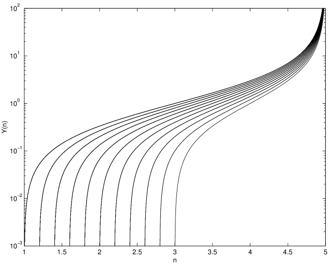
Figure 1: $Y={\dot{\Omega}_{gw}\over{\dot{\Omega}_{em}}}$ as a function of the braking index $n$ for different values of the electromagnetic braking index $n_{em}$. $n_{em}$ varies in the range $[1,3]$ with step 0.2.

We see that a braking index less than 3 can be obtained combining the effects of the electromagnetic and gravitational torques. For instance, for the Crab pulsar we have $n=2.51$ and if we assume, say, $n_{em}=2.4$, then it immediately follows $Y\simeq 0.04$, that is the gravitational radiation contribution to the spin-down rate is about $4\%$ of the electromagnetic one. On the other hand, if $n_{em}=1$, then $Y\simeq 0.6$.

The spin-down of a pulsar in which both the electromagnetic and gravitational torques are acting, Eq.(13), can be expressed as

$$\dot{\Omega}=K_{eff}(\Omega)\times\Omega^{n(\Omega)}$$ (20)

where both the “effective” $K_{eff}$ and $n$ are function of the angular velocity $\Omega.$ As a consequence of its dependence on $\Omega$, the braking index $n$ is not constant in time. In the next section we will derive the time evolution of $n$. In all subsequent calculations we will assume the pulsar momentum of inertia being equal to the canonical value $I=10^{38}\leavevmode\nobreak\ kg\leavevmode\nobreak\ m^{2}$.

From Eq.(14) we can express the ellipticity of the pulsar as

$$\epsilon=1.9\times 10^{5}\sqrt{P^{3}\dot{P}_{gw}}$$ (21)

Combining Eqs.(14,17) we can re-write Eq.(21) as a function of the observed pulsar period and its derivative, and of the ratio $Y$ between the gravitational and electromagnetic spin-down rates:

$$\epsilon=1.9\times 10^{5}\sqrt{P^{3}\dot{P}{Y(n)\over{1+Y(n)}}}=7.55\times 10^{6}\sqrt{{|\dot{\Omega}|\over{\Omega^{5}}}{Y(n)\over{1+Y(n)}}}$$ (22)

Eq.(22) plays a basic role in the determination of the upper limits of the pulsars ellipticity.

4 Pulsar parameters evolution

Differentiating Eq.(17) we easily find

$$\dot{Y}=(5-n_{em})Y{\dot{\Omega}\over\Omega}$$ (23)

and then

$$Y(\Omega)=Y_{0}\left({\Omega\over\Omega_{0}}\right)^{5-n_{em}}$$ (24)

where $Y_{0}={{n_{0}-n_{em}}\over{5-n_{0}}}$, being $n_{0}$ the observed braking index (i.e. its present value). We use this solution to solve the equation for the time evolution of the pulsar angular velocity. To this purpose, let us write Eq.(13) in the form

$$\dot{\Omega}=K_{gw}\Omega^{5}\left({1+Y(\Omega)\over{Y(\Omega)}}\right)$$ (25)

We numerically solve this differential equation, fixing the pulsar age $t_{age}$ and finding a solution depending on three unknowns: the ellipticity $\epsilon$ (contained in $K_{gw}$), $n_{em}$ (on which $Y(\Omega)$ depends) and the initial angular velocity $\Omega_{i}$ ($\Omega_{i}=\Omega(t_{age})$). These quantities must be chosen in order to verify two conditions: those given by $\Omega(t=0)=\Omega_{0}$ and by Eq.(22), calculated for the values of the parameters at $t=0$:

$$\epsilon=7.55\times 10^{6}\sqrt{{|\dot{\Omega}_{0}|\over{\Omega^{5}_{0}}}{Y_{0}\over{1+Y_{0}}}}$$ (26)

This gives us a range of acceptable values for the unknowns. The solution we are searching for is that corresponding to the smallest possible value of electromagnetic braking index $n_{em}$, that is to the greatest value of the ellipticity $\epsilon$. Once we have determined the function $\Omega(t)$ for a given pulsar, we can use Eq.(16) and find the time evolution of the braking index $n(t)$.

In some cases, we can further reduce the range of variation of $n_{em}$ considering the pulsar age, in the following way. Let us consider the ratio $R$ between $\dot{\Omega}_{em}$ and the total spin-down rate, given by Eq.(25), or equivalently, by

$$\dot{\Omega}=K_{em}\Omega^{n_{em}}\left(1+Y(\Omega)\right)$$ (27)

We have

$$R(\Omega)={\dot{\Omega}_{em}\over{\dot{\Omega}}}={1\over{1+Y(\Omega)}}$$ (28)

This quantity varies monotonically between the two limits $R_{inf}=R(\Omega_{i})$ and $R_{sup}=R(\Omega_{0})={{5-n_{0}}\over{5-n_{em}}}\leq 1$. The condition $\dot{\Omega}_{em}\leq R_{sup}\dot{\Omega}$ implies

$$R_{sup}\geq{t_{age}\over\tau_{em}}$$ (29)

with $\tau_{em}$ given by Eq.(11). We choose the range of $n_{em}$ in order to satisfy Eq.(29). In this way, with the exception of the Vela pulsar, we can increase the lower limit of $n_{em}$ then reducing the upper value of $\epsilon$.

In the following we consider individually the four pulsars with measured braking index, applying to each of them the procedure described.

4.1 Crab

The Crab pulsar present parameters are $n_{0}=2.51\pm 0.01$, $\Omega_{0}=188.12\leavevmode\nobreak\ s^{-1}$ and $\dot{\Omega}_{0}=-2.42\times 10^{-9}s^{-2}$, while its age is $t_{age}\simeq 945\leavevmode\nobreak\ yr$. The initial rotation period of the Crab is not exactly known but a value $P_{i}\in[10,20]\leavevmode\nobreak\ ms$ is usually assumed. By solving Eq.(25), under the various conditions previously described, we find $n_{em}\geq 1.7$, $\epsilon\leq 3.8\times 10^{-4}$, $\Omega_{i}\leq 394\leavevmode\nobreak\ s^{-1}$ ($P_{i}\geq 16\leavevmode\nobreak\ ms$). A more tightening limit can be obtained considering that the observed braking index appears to be constant within $0.5\%$ in more than twenty years of observations, thus implying $|\dot{n}|<5\times 10^{-4}\leavevmode\nobreak\ yr^{-1}$ (Lyne et al. lyne1 (1993)). This relation is satisfied if $n_{em}\geq 2.05$ and correspondingly we find $\epsilon\leq 3\cdot 10^{-4}$, $2.5$ times lower than the maximum ellipticity calculated under the hypothesis that the pulsar spin-down is due only to the emission of gravitational waves (Haensel haens (1995)), (Giazzotto et al. giazo (1997)), $\Omega_{i}\leq 364\leavevmode\nobreak\ s^{-1}$ ($P_{i}\geq 17.2\leavevmode\nobreak\ ms$) and $Y_{0}\leq 0.18$.

4.2 Vela

The Vela pulsar is characterized, at present, by $n_{0}=1.4\pm 0.2$, $\Omega_{0}=70.36\leavevmode\nobreak\ s^{-1}$ and $\dot{\Omega}_{0}=-9.85\times 10^{-11}\leavevmode\nobreak\ s^{-2}$. Its age is not well determined but estimates, based on the position offset and the proper motion of the pulsar, give values in the range $[18,31]\times 10^{3}\leavevmode\nobreak\ yr$ (Aschenbach et al. asche (1995)). Assuming $t_{age}=1.8\times 10^{4}\leavevmode\nobreak\ yr$, we have $n_{em}\geq 1.27$, $\epsilon\leq 3.3\times 10^{-4}$, about $5.5$ times lower than the limit relative to the case of gravitational torque alone, $\Omega_{i}\leq 391\leavevmode\nobreak\ s^{-1}$ ($P_{i}\geq 16.1\leavevmode\nobreak\ ms$) and $Y_{0}\leq 0.036$. If $t_{age}=3.1\times 10^{4}\leavevmode\nobreak\ yr$ we find much more tightening limits: $n_{em}\geq 1.399$, $\epsilon\leq 3\times 10^{-5}$, about $60$ times lower than the limit relative to the case of gravitational braking alone, together with $\Omega_{i}\leq 594\leavevmode\nobreak\ s^{-1}$ ($P_{i}\geq 10.6\leavevmode\nobreak\ ms$) and $Y_{0}\leq 2.78\cdot 10^{-4}$.

4.3 PSR 0540-69

The pulsar $PSR\leavevmode\nobreak\ 0540-69$ is characterized by $n_{0}=2.28\pm 0.02$, $\Omega_{0}=124.66\leavevmode\nobreak\ s^{-1}$ and $\dot{\Omega}_{0}=-1.185\times 10^{-9}\leavevmode\nobreak\ s^{-2}$. We do not know exactly its age which, however, should be of about $900\leavevmode\nobreak\ yr$ (Muslimov $\&$ Page musli (1996)). We find $n_{em}\geq 2.21$, $\epsilon\leq 2.4\times 10^{-4}$, which is $6.3$ times lower than the “gravitational” limit, $\Omega_{i}\leq 175\leavevmode\nobreak\ s^{-1}$ ($P_{i}\geq 36\leavevmode\nobreak\ ms$) and $Y_{0}\leq 0.026$.

4.4 PSR 1509-58

The pulsar $PSR\leavevmode\nobreak\ 1509-58$ parameters are: $n_{0}=2.837\pm 0.001$, $\Omega_{0}=41.7\leavevmode\nobreak\ s^{-1}$ and $\dot{\Omega}_{0}=-4.25\times 10^{-10}\leavevmode\nobreak\ s^{-2}$. If the pulsar birth is identified with the supernova event $AD\leavevmode\nobreak\ 185$, then its age is $t_{age}\simeq 1800\leavevmode\nobreak\ yr$ (Thorsett thors (1992)), (Muslimov $\&$ Page musli (1996)). On the other hand its “electromagnetic” age is $\tau_{em}\leq 1700\leavevmode\nobreak\ yr$. The origin of this discrepancy has not been understood yet. So, our model cannot be applied because the pulsar age resulting from the action of both the gravitational and electromagnetic torques is always less than $\tau_{em}$ and cannot match $t_{age}$.

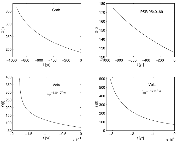
Figure 2: The angular velocity $\Omega(t)$ is plotted as a function of time, assuming $n_{em}$ equal to its lower limit. For the Vela pulsar age both the lower and the upper limit have been considered.

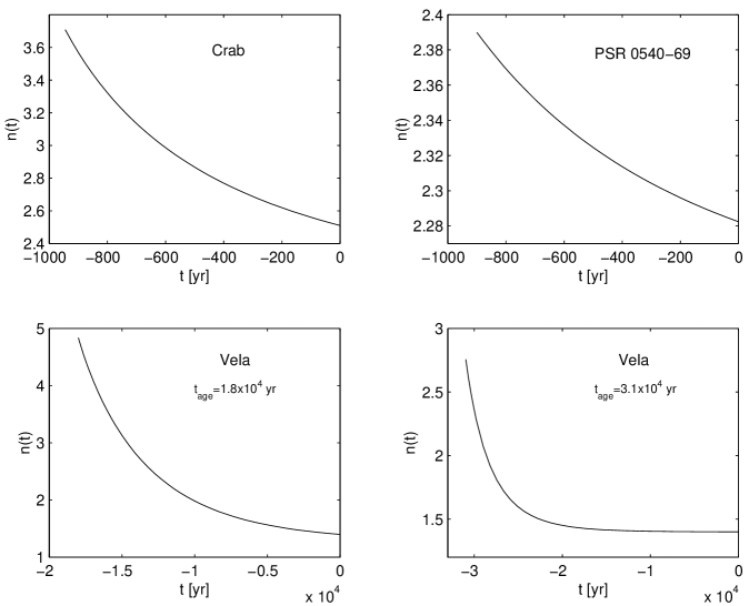
Figure 3: The braking index $n$ is plotted as a function of time, assuming $n_{em}$ equal to its lower limit. For the Vela pulsar age both the lower and the upper limit have been considered.

We have plotted the time evolution of the pulsars angular veocity $\Omega(t)$ in Fig.(2) and that of the braking index $n(t)$ in Fig.(3). In all cases $n(t)\rightarrow n_{em}$ asymptotically, because the gravitational contribution to the spin-down rate decreases faster than the electromagnetic one, see Eq.(17).We note that for the Vela pulsar, if $t_{age}=1.8\cdot 10^{4}\leavevmode\nobreak\ yr$, the initial value of the braking index $n$ could be as high as $4.8$. This implies that $Y_{i}\equiv Y(\Omega_{i})\leq 22$, so that at the beginning the spin-down could have been dominated by the gravitational braking. From the figure we see that $Y$ would have become less than $1$ about $3000\leavevmode\nobreak\ yr$ after the birth. Also for the Crab the gravitational braking could have been dominant at the birth ($Y_{i}\leq 1.28$).

Our results, together with some pulsars parameters, are summarized in Tab.(1).

5 Emission of gravitational waves

From the calculated upper limits on the ellipticity of pulsars we can very easily find new upper limits also on the amplitude of the gravitational signals emitted by them. For a deformed neutron star rotating around a principal axis of inertia, the waveforms corresponding to the two independent polarization states are, in the quadrupole formalism,

$$h_{+}={h_{0}\over 2}\cos{2\Omega t}\left(1+\cos^{2}{\theta}\right)$$ (30)

$$h_{\times}=h_{0}\sin{2\Omega t}\cos{\theta}$$ (31)

where $\theta$ is the angle between the rotation axis of the star and the line of sight and the amplitude $h_{0}$ is given by

$$h_{0}=1.05\times 10^{-27}\left({I\over{10^{38}kg\leavevmode\nobreak\ m^{2}}}\right)\left({10\leavevmode\nobreak\ kpc\over r}\right)\times$$

$$\leavevmode\nobreak\ \leavevmode\nobreak\ \leavevmode\nobreak\ \leavevmode\nobreak\ \times\left({\epsilon\over{10^{-6}}}\right)\left({\nu\over{100\leavevmode\nobreak\ Hz}}\right)^{2}$$ (32)

being $\nu={\Omega\over{\pi}}$ the frequency of the wave, equal to two times the rotation frequency of the star. For completeness, we remember that the power emitted through gravitational waves is

$${dE\over{dt}}=-{32\over{5}}{G\over{c^{5}}}I^{2}\epsilon^{2}\Omega^{6}$$ (33)

In Tab.(1) we have reported, among the other quantities, the maximum amplitude of the gravitational waves emitted from the pulsars with known braking index, calculated by the use of Eq.(32), assuming $I=10^{38}\leavevmode\nobreak\ kg\leavevmode\nobreak\ m^{2}$.

$$r\leavevmode\nobreak\ [kpc]$$

Table 1: Parameters of pulsars: $r$ is the pulsar distance, $P_{0}$ is the measured period, $\nu$ is the frequency of the gravitational waves emitted (twice the orbital frequency), $P_{i,min}$ is the minimum initial period, $Y_{0,max}$ is the maximum present value of the ratio between the gravitational and the electromagnetic contributions to the pulsar spin-down rate, $\epsilon_{max}$ and $h_{max}$ are, respectively, the maximum ellipticity and the maximum amplitude of the gravitational waves emitted. For the Vela pulsar two ages, $t_{age}=1.8\times 10^{4}\leavevmode\nobreak\ yr$ (a) and $t_{age}=3.1\times 10^{4}\leavevmode\nobreak\ yr$ (b) have been considered.

6 Conclusions

Usually, the upper limits on pulsars ellipticity are calculated assuming that pulsar spin-down is due only to the emission of gravitational waves. It is well known that this assumption contradicts the measure of the braking index, which has been obtained for a small sample of pulsars, with values always less than 3.

In this paper we show that considering the simultaneous action, in a pulsar, of a gravitational torque and an electromagnetic one, the observed braking indexes can be recovered. The gravitational torque is always a small correction to the total torque acting on the pulsar. A consequence of the model is that the braking index is not constant in time. We calculate the time evolution of the pulsars angular velocities and braking indexes and find more tightening upper limits to their ellipticity. These new limits are between $2.5$ and $60$ times lower than the old one. New upper limits on the amplitude of the gravitational waves emitted immediately follow.

- (1) Allen, M. P. & Horvath, J. E., 1997, MNRAS 287, 615
- (2) Allen, M. P. & Horvath, J. E., 1997, accepted for publication in ApJ
- (3) Aschenbach, B., Egger, R. & Trumper, J., Nature 373, 587
- (4) Blandford, R. D. et al., 1983, MNRAS, 204, 1025
- (5) Blandford, R. D. & Romani, R. W., 1988, MNRAS 234, 57
- (6) Boyd, P. T., van Citters, G. W., et al., 1995, ApJ 448, 365
- (7) Camilo, F., 1996, in IAU Colloquium 160, Pulsars: Problems and Progress, eds. S. Jonston, M. A. Walker, M. Bailes (ASP Conf. Ser. 106), San Francisco, 39
- (8) Cheng, A. F., 1989, ApJ 337, 803
- (9) Giazzotto, A. et al., 1997, Phys. Rev. D 55, 2014
- (10) Goldreich, P. & Julian, W. H., 1969, ApJ 157, 869
- (11) Haensel, P., 1995, Lecture delivered at Les Houches Summer School, eds. J.-A.Marck and J.-P.Lasota
- (12) Link, B. & Epstein, R., 1997, ApJ 478, L91
- (13) Lyne, A. G., Pritchard, R. S., et al., 1996, Nature 381, 497
- (14) Lyne, A. G., Pritchard, R. S., Smith, F. G., 1993, MNRAS 265, 1003
- (15) Kaspi, V.M., Manchester, R. N., et al., 1994, ApJ 422, L83
- (16) Manchester, R. N. & Taylor, J. H., 1977, Pulsars (San Francisco: W. H. Freeman)
- (17) Muslimov, A. & Page, D., 1996, ApJ 458, 347
- (18) Ostriker, J. P. & Gunn, J. E., 1969, ApJ 157, 1395
- (19) Shapiro, S. L. & Teukolsky, S. A., 1983, Black Holes, White Dwarfs and Neutron Stars, (New York: John Wiley)
- (20) Strom, R. G., 1994, MNRAS, 268, L5
- (21) Thorsett, S. E., 1992, Letters to Nature, 356, 690