Unpulsed Optical Emission from the Crab Pulsar

Abstract

Based on observations of the Crab pulsar using the TRIFFID high speed imaging photometer in the $UBV$ bands using the Special Astrophysical Observatory’s 6m telescope in the Russian Caucasus, we report the detection of pronounced emission during the so-called ‘off’ phase of emission. Following de-extinction, this unpulsed component of emission is shown to be consistent with a power law with an exponent of $\alpha$ = -0.60 $\pm$ 0.37, the uncertainty being dominated by the error associated with the independent CCD photometry used to reference the TRIFFID data. This suggests a steeper power law form than that reported elsewhere in the literature for the total integrated spectrum, which is essentially flat with $\alpha$ $\sim$ 0.1, although the difference in this case is only significant at the $\leq$ 2$\sigma$ level. Deeper reference integrated and TRIFFID phase-resolved photometry in these bands in conjunction with further observations in the $UV$ and $R$ region would constrain this fit further.

1 Introduction

The Crab pulsar provides one of the best multiwavelength sources of magnetospheric emission from $\gamma$-rays to the radio regime and as such, remains the gold standard as regards providing definitive empirical datasets with which to constrain current existing theoretical models of such nonthermal emission. Throughout this entire frequency range, the pulsar’s light curve retains essentially the same morphology, being traditionally divided up into four distinct regions - the two peaks, the Bridge of emission between the peaks, and the ‘off’ region. This latter component was historically presumed to originate from the nebula, a reasonable assumption considering the intense beaming observed from this object.

Optically, the pulsar has been scrutinized ever since its initial discovery in the radio by Staelin & Reifenstein (1968). The pulsar is bright enough for effective single-pixel high speed photometry, and following its confirmation as an optical pulsar by Cocke et al. (1969), numerous such observations followed (e.g. Wampler et al. 1969, Kristian et al. 1970, Cocke and Ferguson 1974, Groth 1975a, Groth 1975b). These observations typically spanned the $BVRI$ wavebands at time resolutions of $\sim$ milliseconds, and as absolute reference timing was not possible, individual light curves per dataset were typically co-added in a least-squares fashion.

Despite the somewhat restricted data acquisition and analytical conditions associated with these observations, there was a consensus that the common arrival time of all these colored peaks was accurate to within 10$\mu$s, there were suggestions of morphological differences between the leading and trailing edges of various light curves, and that the light curve was strongly polarized as a function of rotational phase (Wampler et al. 1969).

Subsequent observations by Peterson et al. 1978 using a 2 dimensional (2-d) image photon counting camera in the $UB$ bands suggested that the supposed ‘off’ phase of the pulsar’s rotational phase was in fact consistent with continuing emission from the pulsar, indicating the Crab was actually ‘on’ for the full rotational cycle. Whilst these results at the time were unprecedented, deeper exposures combined with more rigorous image processing algorithms would have yielded more accurate estimates of the ‘off’ components flux yields and overall spectral form.

In Jones et al. 1981, Smith et al. 1988 and Smith et al. 1996, several dedicated phase-resolved $V$ & $UV$ polarimetric observations of the Crab pulsar using both ground based single-pixel photometers and the $HST$ High Speed Photometer yielded data indicating sharp swings in polarisation angle around both the peaks, in addition to some form of polarisation evolution in the Bridge region. Remarkably, the analysis also indicated a large polarisation component associated with the traditional ‘off’ phase of emission. The inference was that, combined with the earlier Peterson et al. results, the ‘off’ emission of the pulsar was consistent with some form of nonthermal, undoubtedly synchrotron related origin. However, the single-pixel based nature of these observations limited the possibility of accurately resolving the unpulsed component’s contribution in terms of polarisation, which may be expected to contain a substantial nebular component.

Ideally, one requires a high speed 2-d photometer in order to obtain acceptably significant signal to noise (S/N) datasets in several wavebands from which one might hope to photometrically isolate the various components of a phase-resolved light curve. With such systems, the effective photometer sky aperture can be reduced compared with conventional photometers, and effects such as telescope wobble can be entirely removed (Shearer et al. (1996)). Thus, photons chosen for analysis can be selected in software which can place an aperture matched (to maximise S/N) to the prevailing seeing and background conditions, and then isolate those barycentred photons within specifically chosen phase regions of the light curve. The TRIFFID high speed photometer, previously used in the detection of pulsations from both Geminga (Shearer et al. (1998)) and PSR B0656+14 (Shearer et al. (1997)) is ideal in this regard, as it makes use of a MAMA camera. In this communication we document the first attempts to photometrically isolate the Crab’s unpulsed ‘off’ component of emission in three color bands.

2 Observations and Analysis

Observations of the Crab pulsar were made over 5 nights between the 14th and 19th of January 1996, using the TRIFFID camera mounted at Prime Focus of the 6m telescope of the Special Astrophysical Observatory located in the Russian Caucasus. The primary targets of this observing run were the Geminga and PSR B0656+14 pulsars, thus the Crab observations were somewhat limited. Data was taken in the $U$, $B$ and $V$ Johnson bands. The plate scale was 0.22”/pixel at the $MAMA$ photocathode. For all nights observing the Crab, the atmospheric stability was good although there were several transits of high altitude cirrus. Table 1 shows a log of the observations. Each individual dataset was binned to form an integrated image, and from this, reference stars were chosen as guides for the image processing software. Flat fields were prepared using deep dome flats co-added with a number of sky flats, taken immediately after the observations. Image processing, incorporating a Weiner filter modified shift-and-add algorithm (Redfern et al. (1993)), followed, incorporating the derived flat field and correcting for telescope wobble and gear drift. This yielded full field images of the inner Crab nebula within which the pulsar and its stellar companions were registered.

For each dataset, all photons within a radius of 50 pixels of the Crab pulsar were extracted using the image processing software, and these time-stamps were then barycentred using the JPL DE2000 ephemeris. A standard epoch folding algorithm was used to prepare light curves based upon given Jodrell Bank Crab Ephemeris (Lyne & Pritchard, (1996)) via folding modulo the barycentred time series. This yielded both light curves and a phase-resolved image within a certain specfied phase range - in this initial case the full cycle. The number of phase bins used was 3000, yielding a bin resolution of $\sim$ 11 $\mu$s.

Following this, the s2 ($V$), s1 ($U$) & w4 ($B$) images were used respectively as ‘templates’ with which to re-orientate the other color datasets geometrically, so as to result in a set of identical integrated images for each dataset. Total summed errors in this shift-and-rotation technique were of order 0.1$\%$ in terms of pixel units typically. For each colour band, each dataset was summed chronologically, yielding a total $U$, $B$ and $V$ dataset.

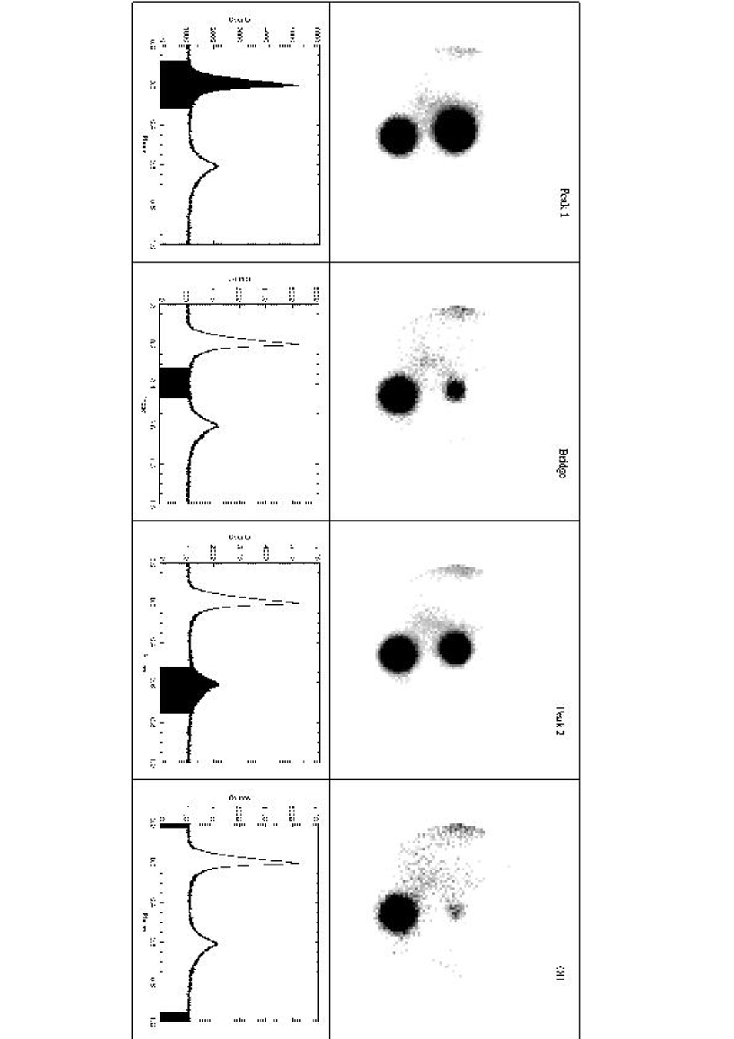
Figure 1: Phase-resolved 2-d photometry of the inner Crab nebula in the $B$ band, taken within a radius of 50 pixels, the pulsar being the centre star. The location of each phase region is indicated in the light curve obtained from a radius of 15 pixels from the Crab centroid, with the accompanying photometric image.

Phase-resolved images obtained based upon the approximate locations of the four principal morphological regions previously defined were obtained as shown in Figure 1. In this figure, the phase regions defining the peaks and Bridge of emission match those defined previously by Eikenberry & Fazio 1997. It is clear that there is emission associated with the pulsar during what has been conventionally regarded as the ‘off’ phase - as had been originally indicated by Peterson et al. With these deep phase-resolved images, it is possible to apply the full arsenal of image processing techniques, and thus photometrically characterise the time-resolved nature of the pulsar’s emission particulary for the ‘off’ region.

In order to do this, we must satisfactorily isolate the unpulsed component from the background-removed light curves, in such a way so that we are satisfied that our denominated phase window samples what is consistent with an unpulsed component only. To isolate this ‘off’ region, standard image processing techniques were used to remove the Crab pulsar from each of the full cycle images in the $UBV$ bands. In effect, one fits an analytical point spread function (PSF) to the full cycle photometric image, and one then uses this PSF to firstly derive the flux associated with full cycle image, and then to derive the fluxes associated with the other phase resolved images corresponding to the two peaks, the bridge and the unpulsed component of emission. We now outline the approach in more detail.

For a given color band, the removal of the Crab pulsar from the full cycle image was performed via the daophot IRAF package, using the psf task to fit a PSF to the Crab pulsar stellar point source. This was then used as in input to the allstar task, which re-fits the PSF to the candidate stellar point source - in this first case, the full cycle Crab image - in order to accurately remove the candidate and in so doing, determine both the flux and its error associated with this procedure. For the full cycle image, the removal was performed satisfactorily, as the deep exposures in $UBV$ provided good background statistics to the required fitting algorithms.

Using standard aperture photometry, the resulting Crab-removed image was then used to determine the total background flux within the fixed radius centred on the PSF derived centroid of the Crab point source. This net background flux was then used to correct the existing light curves. The procedure was repeated for each of the three color band datasets. In each case, the resulting light curve indicated evidence for residual emission during the presumed ‘off’ phase of emission, as can be seen in Figure 1.

It is clearly necessary to determine the duration of the true ‘off’ phase of emission, namely that consistent with emission from a constant source. Perhaps more critically, we want to ensure that this emission is not contaminated by the flux associated with the trailing edge of Peak 2 and the leading edge of Peak 1. In order to do this, we attempted to isolate that part of the corrected light curve within this ‘off’ phase region whose phase-average flux is, to first order, consistent with a constant source of emission. This was done by starting with the largest phase range in terms of bins defining the traditional ‘off’ region, computing the total flux within this range, and then determining the idealised average flux level per bin. The deviation over the defined phase region of the observed flux levels per bin against the averaged flux levels per bin were examined using a $\chi^{2}$ test. This process was repeated iteratively, by dropping the test phase region window (and hence number of bins), and sweeping this through the initially denominated ‘off’ phase region. In this way, at the 95$\%$ level of confidence, the chosen bin range was (0.75 - 0.825) of phase, based on an analysis of the three color band light curves. Within this phase region we are satisfied that the observed flux is consistent with emission from a constant source, at this confidence level. We note that this bin range is marginally smaller than that defined by Percival et al. 1993, on analysis of High Speed Photometer data taken of the Crab pulsar from the Hubble Space Telescope, using a similar analytical technique.

With this ‘off’ region so defined, the corresponding 2-d images were acquired for the three color bands. Application of the IRAF allstar task using the empirically derived full cycle PSF for each of the $UBV$ images successfuly removed the faint stellar point source visible in each, and from this the flux was estimated. In addition, a local PSF was constructed per phase-resolved image, and the fitting-and-extraction process was performed using both local and full-cycle determined PSFs. This was done for completeness, although the full cycle PSF were found to be sufficient and more ideal, being based upon a higher S/N source and substantially diminished background noise (in comparison to the phase-resolved images). This would seem to indicate that sharp nebular features which might be expected to ”contaminate” the off pulse PSF more than that of the on pulse PSF do not contribute significantly to these results.

The original removal and estimation of the relative fluxes from the full cycle $UBV$ datasets yielded a set of reference count rates. All subsequent flux estimates for specific phase regions were subsequently normalized to these reference count rates per color band. Limited prior observations of several Landolt reference stars in the PG0220 field (Landolt (1992)) provided calibration magnitudes which indicated integrated Crab fluxes in agreement with that expected. Using the $UBVR$ ground-based fluxes of Percival et al. 1993 as reference points, we thus renormalized our previously determined fractional fluxes. This reference data was based on ground based observations of the Crab pulsar made at the 2.1m telescope at McDonald Observatory in January 1992, and corrected for interstellar extinction using $E(B-V)$ = 0.51 $\pm$ 0.04 (Savage & Mathis 1978).

Table 2 details this phase averaged flux, and in Table 3 we show the derived fractional fluxes for that of the unpulsed components as determined by this analysis in addition to the other light curve components. In Table 4 we have reproduced the estimated power-law parameter $\alpha$ determined via a weighted least-squares analysis of each individual spectral dataset. We have re-calculated $\alpha$ for the both the full range & $UBV$ Percival et al. dataset to compare with the other power-law fits. We note that one would estimate a change in flux of $\sim$ 0.01 over the four years between the reference integrated flux and our observations, following the phenomenologically derived $\dot{L_{V}}$ $\sim$ 0.003 mag/yr (Pacini (1971)), empirically confirmed most recently by Nasuti et al. (1997), which is within the error bounds quoted.

3 Discussion

The question of the unpulsed component of emission for the Crab pulsar has always remained somewhat challenging, as one is confronted with temporal problems and the nebular contribution. With this 2-d $MAMA$ data, definitive flux estimates are attainable for the first time. In Peterson et al. 1978, (and elsewhere Miller & Wampler, 1969), the estimated total unpulsed emission is compared with the peak intensity - rather a relative area in terms of phase allocation at our level of temporal resolution - and also with mean pulsed flux. Peterson et al. applied rather novel techniques in the image processing their data obtained via the use of a 6.2ms time resolved Image Photon Counting System camera. Using an iterative least-squares semi-empirical based PSF, they determined residuals which when smoothed yielded a background image which was subtracted from the star field, and the same method estimated the star intensities. Peterson et al. did not present errors associated with their eventual tabulated results. We note the 6.2ms absolute timing resolution. This is some $\sim$ 20$\%$ of the light curve, and accurate phase resolution may not have guaranteed accurate continual phase resolution photometry. Timing errors, accurate phase resolution and estimation of the total aperture background are all guaranteed at unprecedented resolution with our datasets. From the background corrected light curves, we can determine the incident flux within the designated ‘steady’ region of emission, and then compare it directly with both the total pulsar flux and pulsed-only flux. These differences, presented in terms of magnitude change, are shown in Table 5.

The tabulated data suggests that the original estimates by Peterson et al. 1978 were optimistic by typically at least a magnitude, but this is understandable bearing in mind the rather difficult data and analysis they were working with. There is agreement to some extent with the trend - the early datasets suggested that there was a greater ratios in the $B$ in comparison to the $U$ band, yet no error estimates are included. No $V$ data was analysed at that time. We note that if one was to assume that the unpulsed emission was restricted to a specfic phase region, and not assumed to exist for the entire rotation, then whilst the ratios would drop further, they would still imply a similar spectral form.

In Figure 2 we reproduce the full Percival et al. (1993) derived corrected flux distribution with the unpulsed flux estimates implied from the tabulated ratios. We have also included the derived flux fractions for peaks 1 and 2, and the Bridge of emission, which are considered elsewhere in some detail (Golden et al., 1999). It seems clear that one can represent the unpulsed emission in spectrally in terms of a steeper power-law with $\alpha$ $\sim$ -0.60 $\pm$ 0.37 in contrast to the rather flat $\alpha$ $\sim$ 0.11 $\pm$ 0.08 associated with the full integrated emission.

4 Conclusion

The resolved unpulsed flux component, whether within its defined ‘off’ region or normalized to the pulsar’s full cycle, suggests a power-law form. There are two options - either the emission is real and of a nonthermal nature or the emission is false, a consequence of some form of photocathode or other artifact intrinsic to the $MAMA$ photon counting detector. This latter would manifest timing irregularities which were not evident under analysis. Photon timeseries taken from the pulsar and other stars in the field were tested for deviations from a Poissonian distribution at varying timescales, and there was no evidence for such a deviation at the 99% confidence level, atmospheric variations notwithstanding. In this, we confirm the earlier work of Smith et al. (1978). Consequently we may conclude that the emission is from the pulsar.

This unpulsed emission has been more commonly observed in the higher (X-ray & $\gamma$-ray) regimes, and scrutinised in some detail. In X-rays, the unpulsed component is difficult to discern amid the intense nebular emission. Becker & Aschenbach 1995 attempted to analyse $ROSAT$ HRI data, ostensibly to determine limits to the pulsar’s thermal emission during the unpulsed phase - they concluded with a realistic upper limit to $T_{surface}$ for the Crab’s temperature. This does seem to suggest that in X-rays, the hot Crab and the plerion would dominate the emission.

For detected unpulsed $\gamma$-ray emission, the existing models place the emission either just beyond the magnetosphere or far out in the plerion, namely the Outer-Gap model of Cheung $\&$ Cheng 1994, and the pulsar-wind model of De Jager $\&$ Harding 1992. Two principle predictive facts concern us regarding these two models; the first is that the Pulsar-Wind model implies an emission region large in extent, perhaps up to $\sim$ 20”, whereas the Outer-Gap model requires emission to occur in the immediate vicinity of the pulsar, thus having a resolution of order $\ll$ 1”. Secondly, the Outer-Gap model implicitly expects a correlation between the pulsed and unpulsed emission, whether it be temporal or spectral in nature (Cheung $\&$ Cheng 1994).

Based upon our resolved functional form for the unpulsed component we can reject the De Jager & Harding model, as the source is undeniably localised to the pulsar. The conclusion is that the emission is in some way magnetospherically related. We cannot accept the opposing Cheng & Cheung model for a number of reasons. The emission mechanism is based on the original outer-gap magnetospheric model Cheng, Ho & Ruderman, (1988), and in this case is a result of the cross-streaming of two opposing outer-gaps primary & secondary photon streams. Here the inner streaming IR-optical photons from the far-side gap collide with the primary $\gamma$-rays & e^± pairs from the near-side gap at some distance ($\sim$ 3$R_{LC}$) from the magnetosphere. These interactions result in isotropically radiated high energy emission, predominately from X-rays (MeV) to $\gamma$-rays (Gev – TeV). Cheung & Cheng 1994 point out that at the low (keV - 50 MeV) range, their model predicts flux levels much lower than that observed, and that other mechanisms not accounted for (they suggest synchrotron self-Compton mechanisms) must be present. It is clear that any IR-optical photons that are emitted will be predominately pulsed in nature (as in the original Cheng, Ho & Ruderman, (1988) ansatz) as the process advocated would be expected to be preferentially luminous at the higher frequency ranges.

There have been other attempts to explain the observed steady emission (Peterson et al. 1978); they are that

• the unpulsed component is actually pulsed emission emitted from points spatially extended in the magnetosphere, and it is manifested to us following varying time-of-flights and relativistic effects,

• the pulses could actually possess trailing & leading edges that effectively result in fully pulsed emission,

• the unpulsed component is a result of the reprocessing or reflection of pulsed emission from material near the pulsar (such as a nebulosity, localised knot etc.).

The spatially extended hypothesis above is commensurate with the numerical model framework of Romani and Yadigaroglu 1995, which requires that emission occurs from such a similar topology with similar arguments for the resulting formation of the light curve morphologies. However, this model was based on a number of questionable assumptions as noted by the paper’s authors. More critically, Eikenberry & Fazio 1997 have unambigously shown evidence for significant intra-color phase differences between the leading and trailing edges from $\gamma$-rays to the IR, consistent with a localised origin. These caveats have made such a theoretical basis difficult.

We have already noted the similar spectral forms of both the Bridge and unpulsed components of emission as is evident from Table 4. It is our contention that the observed unpulsed component of emission has its source in a similar electron population/magnetic field/Lorentz factor environment to the Bridge component. The change in power-law exponents from the peaks to the Bridge/unpulsed component may be as a result of either a change in the emitting e^± energy distribution or via modification (due to scattering or absorption processes) of the emitted photon flux. In either case this would be consistent with emission occurring from a region closer to the neutron star within the magnetosphere particularly if we were to assume a common e^± energy distribution originating above a polar cap, which would be expected to evolve in this way as the e^± population streams radially along the open field lines. Ultimately whether both Bridge & unpulsed emission are associated with the main peaks, or whether they are spatially & energetically seperate is at this stage unresolved; viewing geometry issues may be a major factor.

We recall from Smith et al. 1988 that the unpulsed component could be regarded as an extended source of emission, spread in longitude in proximity to light cylinder. The observed flux would then be the result of emission from field lines at and beyond the limit of the polar cone regions, including both the leading and trailing edges of the cores. These field lines would be expected to be affected by abberation and tend towards a toroidal direction - Smith et al. 1988 note that the position angle of the unpulsed (and indeed Bridge component) is similar to that of the mean of the peaks, namely $130^{o}$. Thus these unusual polarisation effects noted by Smith et al. 1988 and others indicate similar behaviour for both Bridge & unpulsed regions, perhaps substantiating a belief that they are in some way phenomenologically linked. Another hypothesis is that the observed unpulsed component represents some fraction of the original synchrotron emitting photons scattered by the local $e^{\pm}$ particle density along various path lengths within the magnetosphere, resulting in an apparently isotropically radiated emission component. However, one might expect an essentially randomised polarisation nature to these scattered photons, which is not reflected in previous phase-resolved polarimatory.

Clearly, we require further unpulsed estimates in the $UV$ and $R-IR$ wavebands in order to characterise the manner in which this emission component correlates with that of the dominant pulsed emission - most interestingly in the vicinity of $\sim$ $10^{14}$ Hz, where an apparent rollover inconsistent with conventional synchrotron self-absorption is apparent. Such estimates would provide constraints to the existing power-law fits, consolidating our contention that the unpulsed component of emission is steeper than that for the integrated spectral index. Perhaps of even greater urgency would be the definitive acquistion of polarimetric photometry of the unpulsed component with the nebular content removed so as to finally assess a possible link between it and the Bridge of emission. Such future work could provide yet more critical empirical constraints to the nascent field of numerical magnetospheric optical emission models.

Acknowledgements

The authors wish to thank R. Butler for assistance with the photometric analysis and M. Cullum for provision of the ESO MAMA detector. The support of Enterprise Ireland, the Irish Research and Development agency, is gratefully acknowledged. This work was supported by the Russian Foundation of Fundamental Research, the Russian Ministry of Science and Technical Politics, and the Science-Educational Centre ”Cosmion”, and under INTAS Grant No. 96-0542.

Figure 2: Integrated de-extincted flux estimates for the Crab from Percival et al. 1993 and the derived flux estimates for both the peaks, Bridge and unpulsed component of emission based on the TRIFFID datasets.

Table 1: Summary of Observations January 1996 BTA

Dataset	Date	UTC	Duration (s)	Filter	Seeing (”)
96zd3.0.0	12/1/96	16:38:51	155	V	2”
96zj5.0.0	13/1/96	16:33:50	334	U	1.6”
96zj7.0.0	13/1/96	16:53:36	297	V	1.3”
96zo5.0.0	14/1/96	16:07:36	617	U	1.9”
96zo6.0.0	14/1/96	16:21:41	584	V	1.6”
96zs1.0.0	15/1/96	17:07:34	1502	U	1.5”
96zs2.0.0	15/1/96	17:38:20	1177	V	1.3”
96zt2.0.0	15/1/96	18:48:40	170	V	1.4”
96zv2.0.0	16/1/96	16:37:01	1468	V	1.8”
96zw2.0.0	16/1/96	17:38:01	1811	B	1.6”
96zw3.0.0	16/1/96	18:09:16	920	V	1.4”
96zw4.0.0	16/1/96	18:44:09	1415	B	1.4”
96zx1.0.0	16/1/96	19:08:51	140	V	1.4”
96zx2.0.0	16/1/96	21:15:04	49	B	1.7”
96zx3.0.0	16/1/96	21:20:22	1212	B	1.7”
96zx9.0.0	17/1/96	16:02:33	337	U	1.8”
96zx10.0.0	17/1/96	16:09:51	47	U	1.8”
96zx11.0.0	17/1/96	16:15:32	2709	U	1.9”
96zy1.0.0	17/1/96	17:02:42	1848	V	1.6”
96zy3.0.0	17/1/96	17:39:08	1263	B	1.7”

Table 2: Integrated Flux from the Crab Pulsar (Percival et al. 1993). The third column represents the fractional transmission as a function of the extinction per specific waveband.

Band	Raw Flux Density	Extinction	De-extincted Flux Density
	mJy	Frac. Trans.	mJy
UV	0.11 $\pm$ 0.02	0.031 $\pm$ 0.002	3.4 $\pm$ 0.25
U	0.31 $\pm$ 0.02	0.101 $\pm$ 0.006	3.1 $\pm$ 0.2
B	0.47 $\pm$ 0.02	0.145 $\pm$ 0.009	3.2 $\pm$ 0.2
V	0.73 $\pm$ 0.04	0.227 $\pm$ 0.014	3.2 $\pm$ 0.2
R	0.90 $\pm$ 0.05	0.313 $\pm$ 0.019	2.9 $\pm$ 0.2

Table 3: Fractional Flux derived from Photometric Analysis.

Parameters		Waveband
	U (mJy)	B (mJy)	V (mJy)
Peak 1	2.00 $\pm$ 0.13	1.95 $\pm$ 0.12	1.93 $\pm$ 0.12
Peak 2	1.09 $\pm$ 0.07	1.1 $\pm$ 0.07	1.12 $\pm$ 0.07
Bridge	0.087 $\pm$ 0.006	0.103 $\pm$ 0.006	0.108 $\pm$ 0.007
Off Phase	0.014 $\pm$ 0.002	0.017 $\pm$ 0.002	0.019 $\pm$ 0.002

Table 4: Estimated Spectral Power-Laws from Photometric Analysis

Dataset	Power-Law $\propto$ $\nu^{\alpha}$
Integrated UV/U/B/V/R	0.11 $\pm$ 0.09
Integrated U/B/V	-0.07 $\pm$ 0.18
Peak 1	0.07 $\pm$ 0.19
Peak 2	-0.06 $\pm$ 0.19
Bridge	-0.44 $\pm$ 0.19
Off	-0.60 $\pm$ 0.37

Table 5: Ratios of pulsed/unpulsed emission in magnitudes for $U$, $B$ & $V$. Here, total emission corresponds to the full integrated emission from the pulsar. Full cycle corresponds to the unpulsed emission over 0.075 phase normalised to one cycle.

Ratio	U	B	V
	${\bf This~{}Work}$
total emission/(0.075 phase)	5.8 $\pm$ 0.2	5.6 $\pm$ 0.1	5.6 $\pm$ 0.1
total emission/(full cycle)	3.0 $\pm$ 0.2	2.8 $\pm$ 0.1	2.7 $\pm$ 0.1
	${\bf Peterson~{}et~{}al.}$ 1978
total emission/(full cycle)	1.5	1.6	n/a

References

- Becker & Aschenbach, (1995) Becker, W., & Aschenbach, B., 1995, in The Lives of the Neutron Stars, ed. A. Alpar, U. Kiziloglu, & J. van Paradijs, (Kluwer Academic, Dordrecht, Holland), 47.
- Becker & Truemper, (1997) Becker, W., & Truemper, J., 1997, A&A, 326, 682.
- Cheng, Ho & Ruderman, (1988) Cheng, K.S., Ho, C., & Ruderman, 1986, ApJ, 300, 500, 19.
- Cheung & Cheng, (1994) Cheung W.M., & Cheng K.S, 1994, ApJS, 90, 827.
- Cocke et al. (1969) Cocke, W. J., Disney, M. J. & Taylor, D. J., 1969, Nature, 221, 525
- Cocke & Ferguson, (1974) Cocke, W.J., & Ferguson, D.C., 1974, ApJ, 194, 725, 1974.
- Cullum, (1990) Cullum, M., 1990, The MAMA Detector Users’ Manual, ESO
- De Jager & Harding, (1992) De Jager, O.C., & Harding, A.K., 1992, ApJ, 396, 161.
- Eikenberry & Fazio, (1997) Eikenberry, S.S. & Fazio, G.G., 1997, ApJ, 476, 281.
- Golden (1999) Golden, A., 1999, Ph.D. Thesis, N.U.I., Galway.
- (11) Groth, E.J., 1975a, ApJS, 29, 431.
- (12) Groth, E.J., 1975b, ApJ, 200, 278.
- Jones et al. (1981) Jones, D.H.P., Smith, F.G., & Wallace, P.T., MNRAS, 196, 943, 1981
- Kristian et al. (1970) Kristian, J., Visanathan, N., Westphal, J.A., & Snellen, G.H., 1970, ApJ, 162, 475.
- Landolt (1992) Landolt, A. U., 1992, AJ, 104, 372
- Lyne & Pritchard, (1996) Lyne A. & Pritchard R. S., 1996, Crab Timing Ephemeris, University of Manchester.
- Nasuti et al. (1997) Nasuti, F.P., Mignani, R., Caraveo, P.A., & Bignami, G.F., 1997, A&A, 314, 849.
- Pacini (1971) Pacini, F., ApJ, 163, L17, 1971.
- Percival et al. (1993) Percival, J.W., Biggs, J.D., Dolan, J.F., Robinson, E.L., Taylor, M.J., et al., 1993, ApJ, 407, 276.
- Peterson et al. (1978) Peterson, B.A., Murdin, P., Wallace, P., Manchester, R.N., Penny, A.J., Jorden, A., et al., 1978, Nature, 276, 475.
- Redfern et al. (1993) Redfern, R.M., Devaney, M.N., O’Kane, P., Ballesteros Ramirez, E., Gomez Renasco, R., & Rosa, F., 1993, MNRAS, 238, 791.
- Romani & Yadigaroglu, (1995) Romani, R., & Yadigaroglu, I.-A., 1995, ApJ, 438, 314.
- Savage & Mathis, (1978) Savage, B.D., & Mathis, J.S., 1978, Annual Review of Astronomy and Astrophysics, 17, 73.
- Shearer et al. (1996) Shearer, A., Butler, R., Redfern, R. M., Cullum, M. & Danks, A. C., 1996, ApJ, 473, 115
- Shearer et al. (1997) Shearer, A., Redfern, M., Gorman, G., Butler, R., Golden, A., et al., 1997, ApJ, 487, L181.
- Shearer et al. (1998) Shearer, A., Golden, A., Harfst, S., Butler, R., Redfern, M., et al., 1998, A&A, 335, L21.
- Smith (1971) Smith, F.G., 1971, Nature, 231, 191.
- Smith et al. (1978) Smith, F.G., Disney, M.J., Hartley, K.F., Jones, D.H.P., King, D.J. et al., 1978, MNRAS, 184, 39.
- Smith (1986) Smith, F.G., 1986, MNRAS, 219, 729.
- Smith et al. (1988) Smith, F.G., Jones, D.H.P, Dick, J.S.B., & Pike, C.D., 1988 MNRAS, 233, 305.
- Smith et al. (1996) Smith, F.G., Dolan, J.F., Boyd, P.T., Biggs, J.D., Lyne, A.G., & Percival, J.W., 1996, MNRAS, 282, 1354.
- Staelin & Reifenstein (1968) Staelin, D.H.,& Reifenstein, E.C., 1968, Nature, 183, 1481.
- Wampler et al. (1969) Wampler, E.J., Scargle, J.D., & Miller, J.S., 1969, ApJ, 157, L1.