COSMOS: A Hybrid $N$-Body/Hydrodynamics Code for Cosmological Problems

Abstract

We describe a new hybrid $N$-body/hydrodynamical code based on the particle-mesh (PM) method and the piecewise-parabolic method (PPM) for use in solving problems related to the evolution of large-scale structure, galaxy clusters, and individual galaxies. The code, named COSMOS, possesses several new features which distinguish it from other PM-PPM codes. In particular, to solve the Poisson equation we have written a new multigrid solver which can determine the gravitational potential of isolated matter distributions and which properly takes into account the finite-volume discretization required by PPM. All components of the code are constructed to work with a nonuniform mesh, preserving second-order spatial differences. The PPM code uses vacuum boundary conditions for isolated problems, preventing inflows when appropriate. The PM code uses a second-order variable-timestep time integration scheme. Radiative cooling and cosmological expansion terms are included. COSMOS has been implemented for parallel computers using the Parallel Virtual Machine (PVM) library, and it features a modular design which simplifies the addition of new physics and the configuration of the code for different types of problems. We discuss the equations solved by COSMOS and describe the algorithms used, with emphasis on these features. We also discuss the results of tests we have performed to establish that COSMOS works and to determine its range of validity.

1 Introduction

The study of many problems of interest in astrophysics today benefits from or even requires the use of three-dimensional hydrodynamical or $N$-body simulations because the complex physical processes or the lack of symmetry involved prohibit analytic or reduced-dimensionality approaches. These problems span the entire range of astrophysical length scales, from black hole collisions and core-collapse supernovae to clusters of galaxies and the Lyman $\alpha$ forest. The advent over the past two decades of modern shock-capturing hydrodynamical algorithms and fast $N$-body methods, together with rapid advances in available computing power, has made such simulations feasible.

In these simulations one must make a distinction between collisional matter, in which the mean free path between particle collisions is much smaller than all length scales of interest, and collisionless matter, in which particles may free-stream between collisions on length scales important to the simulation. For collisional matter, a fluid description incorporating a pressure field and a single-valued bulk velocity field is appropriate; shock waves can convert energy irreversibly from bulk kinetic form to internal form. For collisionless matter, the bulk velocity can take on multiple values at each point in space, and shock waves are not possible.

For simulations of galaxies, clusters of galaxies, and large-scale structure it is important to track both kinds of matter. On the length and time scales of interest in these simulations, baryonic matter (the intracluster or intergalactic medium) behaves as a collisional fluid. Although locally this gas may be partially or fully ionized, with collisions between ions and electrons occurring by means of randomly oriented magnetic fields, on resolvable length scales we may assume charge neutrality and ignore local deviations from fluid behavior (e.g., plasma instabilities). However, because we do not yet know the identity of the dark matter, we adopt the simplest hypothesis and assume that it is collisionless. The gravitational stability of apparently bound systems (galaxies and clusters of galaxies) in which baryons provide insufficient mass is still our best evidence for the existence of dark matter. Thus the simplest hypothesis also treats the interaction between these types of matter as purely gravitational. Cosmological simulations must track the evolution of both matter constituents in their mutual gravitational field.

Several codes now exist to simulate the combined evolution of collisional and collisionless matter in a cosmological setting. All treat the dark matter using superparticles which sample the particle distribution. These $N$-body codes differ in the methods they use to compute interparticle forces and to solve the hydrodynamical equations for the gas. Methods for computing interparticle forces include direct summation (PP, or particle-particle), tree algorithms (Hernquist 1987), particle-mesh methods (PM: Hockney & Eastwood 1988), and combinations of direct summation and particle-mesh (P³M: Efstathiou & Eastwood 1981). The tree and particle-mesh algorithms trade off force accuracy or spatial resolution for speed in comparison with direct summation, while variants of P³M attempt to overcome the resolution limitations of PM techniques while retaining their speed.

The hydrodynamic solvers currently in use with particle codes include variants of smoothed-particle hydrodynamics (SPH: Gingold & Monaghan 1977; Lucy 1977) and grid-based methods such as the piecewise-parabolic method (PPM: Colella & Woodward 1984) and the total-variation-diminishing method (TVD: Harten 1983). SPH algorithms descended from astrophysical $N$-body techniques and use particles to approximate the behavior of the gas, treating gas particles as moving interpolation centers for quantities such as the gas pressure. Typically SPH codes achieve good spatial resolution in high-density regions but handle shocks and low-density regions poorly. Examples of cosmological hydrodynamics codes based on SPH include those of Evrard (1988), Hernquist & Katz (1989), Navarro & White (1993), Couchman, Thomas, & Pierce (1995), Steinmetz (1996), and Owen et al. (1998). Grid-based methods, which are used widely in other areas of physics and in engineering, suffer from more limited resolution, but they handle high-density and low-density regions equally well, and with modern algorithms they handle shocks extremely well. Moreover, it is more straightforward to add extra gas physics to grid-based codes. Examples of grid-based cosmological hydrodynamics codes (excluding those based on PPM, which are discussed below) include the centered-difference code of Cen (1992), the TVD code of Ryu et al. (1993), the softened Lagrangian code of Gnedin (1995), and the moving-mesh TVD code of Pen (1998). Comparisons of various cosmological particle- and grid-based codes have been performed by Kang et al. (1994) and Frenk et al. (1999).

The combination of PM for dark matter and PPM for gas has proven to be an especially useful method for cosmological simulations. Accurate shock handling and straightforward implementation of subgrid physics argue for the use of a grid-based scheme for the gas. When using a grid for the gas, the most efficient means for obtaining the forces on the dark matter particles is the particle-mesh method, because the gas and dark matter both make use of the potential defined on the grid. Also, because the gas grid limits the spatial resolution, the greater dynamic range of a tree code or direct summation solver for the dark matter is not as useful. In recent years several groups have independently developed PM-PPM codes to study large-scale structure and galaxy cluster formation (Bryan et al. 1995; Sornborger et al. 1996; Gheller, Pantano, & Moscardini 1998; Quilis, Ibáñez, & Sáez 1996, 98) and cluster evolution (Roettiger, Stone, & Mushotzky 1997). These codes differ in a number of ways. The Bryan et al., Sornborger et al., and Roettiger et al. codes use the Lagrange-plus-remap formulation of PPM, whereas the Gheller et al. code uses the direct Eulerian formulation. Little difference in numerical accuracy between the two formulations has been observed, but the Lagrange-plus-remap formulation generalizes somewhat more readily to moving or adaptive grids. The Bryan et al. code adds certain ad hoc modifications to the basic PPM scheme to improve the resolution of narrow density peaks, and more recently this code has been extended to include adaptive mesh refinement (AMR: Norman & Bryan 1999). The Quilis et al. code makes use of a linearized Riemann solver due to Roe (1981), whereas the other codes use variants of the iterative Riemann solver due to van Leer (1979). All of the codes except that of Roettiger et al. use a Green’s function technique (via the Fast Fourier Transform, or FFT) to solve for the combined gravitational potential of the gas and dark matter. The Roettiger et al. code uses a conjugate gradient solver (Hockney & Eastwood 1988) for the Poisson equation. To our knowledge, all of the codes use cloud-in-cell (CIC) weighting together with a variable-timestep time integration scheme for the particle-mesh code.

We have developed a new PM-PPM code, called COSMOS, for simulations of large-scale structure formation and galaxy cluster evolution. Like Gheller et al. (1998), we use the direct Eulerian formulation of PPM, and like all of the above codes we use CIC weighting and a variable timestep in our PM code. However, our code uses a full multigrid solver rather than an FFT to obtain the gravitational potential, enabling us to handle nonuniform grids with isolated boundary conditions. Also, we have implemented a nonideal equation of state following Colella & Glaz (1985) (of use, for example, in Ly $\alpha$ cloud and supernova simulations), and we implement cooling and multifluid source terms, as well as cosmological expansion terms, with a method similar to that used by Kritsuk, Böhringer, & Müller (1998). The hydrodynamical and gravitational components of COSMOS have been used previously by Ricker (1998) to study purely hydrodynamic cluster evolution, and the full code has been used by Ricker & Sarazin (2000) to simulate cluster mergers including gas and dark matter.

In this paper we describe the COSMOS code and the results of our validation tests. Section 2 discusses the physics included in the code and the corresponding equations. In Section 3 we discuss the discretization scheme used for the grid-based components of the code, the algorithms we use, and the modifications we have made to the standard algorithms to suit the requirements of cosmological problems. Section 4 describes the test problems we have used to validate the code. Finally, Section 5 summarizes the paper.

2 Equations

In this section we describe the definitions and equations used in the COSMOS code. All calculations take place in a three-dimensional computational volume in which positions are specified using comoving coordinates ${\bf x}={\bf r}/a$, where ${\bf r}$ is a proper position vector and $a(t)$ is the time-dependent cosmological scale factor. Both dark matter and gas peculiar velocities ${\bf v}$ are considered to be comoving; thus ${\bf v}=\dot{{\bf x}}$ for a particle at location ${\bf x}$. We define the comoving gas density and pressure as

$${\rho_{\rm g}} = a^{3}\tilde{\rho}_{\rm g}$$ (1)

$$p = a\tilde{p}\ ,$$

where $\tilde{\rho}_{\rm g}$ and $\tilde{p}$ are the proper gas density and pressure, respectively. (We use the subscripts g and dm to distinguish quantities which apply separately to both the gas and dark matter.) Note that our definition of $p$ requires that the comoving internal energy density be given by

$${\rho_{\rm g}}\epsilon=a\tilde{\rho}_{\rm g}\tilde{\epsilon}\ ,$$ (2)

where $\tilde{\epsilon}$ is the proper specific internal energy of the gas. For an ideal-gas equation of state with ratio of specific heats $\gamma$ and average atomic mass $\mu$, we have

$${\rho_{\rm g}}\epsilon={p\over\gamma-1}={{\rho_{\rm g}}kT\over(\gamma-1)\mu}\ ,$$ (3)

where

$$T={\tilde{T}\over a^{2}}$$ (4)

is the comoving temperature, and $\tilde{T}$ is the proper temperature. We also define the comoving potential $\phi$ as the solution at each simulation timestep to Poisson’s equation,

$$\nabla^{2}\phi={4\pi G\over a^{3}}\left[\left({\rho_{\rm g}}+{\rho_{\rm dm}}\right)-\overline{\left({\rho_{\rm g}}+{\rho_{\rm dm}}\right)}\right]\ .$$ (5)

Here ${\rho_{\rm dm}}$ is the comoving density in dark matter particles, and the bar indicates a spatial average. The comoving total energy density of the gas is defined as

$${\rho_{\rm g}}E\equiv{\rho_{\rm g}}\epsilon+{1\over 2}{\rho_{\rm g}}v_{\rm g}^{2}+{\rho_{\rm g}}\phi\ ,$$ (6)

where $v_{\rm g}=|{\bf v}_{\rm g}|$ is the comoving speed of the gas. Finally, for certain problems we make use of an equilibrium cooling function, which we denote by $\Lambda({\rho_{\rm g}},T)$. For example, cooling via optically thin thermal bremsstrahlung emission, assuming a fully ionized gas, would require $\Lambda\propto{\rho_{\rm g}}^{2}T^{1/2}$.

We use these definitions to transform the inviscid Eulerian equations of hydrodynamics into a simple comoving form which, in a static universe ($a\equiv 1$), reduces again to the standard equations with comoving quantities equivalent to proper ones. The comoving gas equations solved by COSMOS are as follows:

$${\partial\over\partial t}{\rho_{\rm g}}+\nabla\cdot\left[{\rho_{\rm g}}{\bf v}_{\rm g}\right]=0$$ (7)

$${\partial\over\partial t}\left({\rho_{\rm g}}{\bf v}_{\rm g}\right)+\nabla\cdot\left[{\rho_{\rm g}}{\bf v}_{\rm g}{\bf v}_{\rm g}\right]+{\bf\nabla}p+2{{\dot{a}\over a}}{\rho_{\rm g}}{\bf v}_{\rm g}+{\rho_{\rm g}}{\bf\nabla}\phi=0$$ (8)

$${\partial\over\partial t}\left({\rho_{\rm g}}E\right)+\nabla\cdot\left[\left({\rho_{\rm g}}E+p\right){\bf v}_{\rm g}\right]+{{\dot{a}\over a}}\left[(3\gamma-1){\rho_{\rm g}}\epsilon+2{\rho_{\rm g}}v_{\rm g}^{2}\right]-{\rho_{\rm g}}{\partial\phi\over\partial t}+\Lambda=0$$ (9)

$${\partial\over\partial t}({\rho_{\rm g}}\epsilon)+\nabla\cdot\left[\left({\rho_{\rm g}}\epsilon+p\right){\bf v}_{\rm g}\right]-{\bf v}_{\rm g}\cdot{\bf\nabla}p+{{\dot{a}\over a}}(3\gamma-1){\rho_{\rm g}}\epsilon+\Lambda=0$$ (10)

The equations are written in explicit conservation form. With the finite-volume discretization used in COSMOS (Section 3.1.1), we can difference these equations (except for the internal energy equation) in such a way that errors in the advection terms do not affect global conservation of mass, momentum, and energy.

We determine which energy equation to use in updating the pressure on the basis of the magnitude of the internal energy density. During a simulation timestep we update the internal energy and pressure according to the internal energy equation (10) and the equation of state (3). We update the total energy using the total energy equation (9). At the end of the timestep, if in any zone the condition

$${\rho_{\rm g}}\epsilon>10^{-2}\max\left\{{1\over 2}{\rho_{\rm g}}v_{\rm g}^{2},|{\rho_{\rm g}}\phi|\right\}$$ (11)

is satisfied, we reset the internal energy density using equation (6) with the updated values of ${\rho_{\rm g}}E$, ${\rho_{\rm g}}$, ${\bf v}_{\rm g}$, and $\phi$, then use the equation of state to reset the pressure. If this criterion is not satisfied, we instead reset the total energy density in that zone using equation (6). This procedure permits us to maintain total energy conservation in regions where the pressure makes a significant contribution to the total energy while avoiding large round-off errors in the pressure where it is small. Condition (11) is generally satisfied except for high Mach-number flows and in ‘dust’ calculations where the gas pressure offers little support against gravity. Similar methods based on energy (Bryan et al. 1995) and entropy (Ryu et al. 1993) are used by other codes to handle such flows.

Equations (7) through (10) suffice to describe the behavior of matter that is collisional on the length scales of interest to us. Examples include the gas in stellar atmospheres and in clusters of galaxies. However, for collisionless matter components, such as galaxies and dark matter in clusters, we must solve the equations of motion for individual particles. These particles are subject only to gravitational forces; hence a particle’s comoving position ${\bf x}_{\rm dm}$ and velocity ${\bf v}_{\rm dm}$ evolve according to

$${d{\bf x}_{\rm dm}\over dt}={\bf v}_{\rm dm}$$ (12)

$${d{\bf v}_{\rm dm}\over dt}+2{\dot{a}\over a}{\bf v}_{\rm dm}=-\nabla\phi,$$ (13)

the second term on the left in the velocity equation representing the Hubble flow due to uniform expansion.

3 Numerical methods

3.1 Hydrodynamics

3.1.1 Finite-volume discretization

We solve the hydrodynamical equations described in Section 2 on a nonuniform, finite, Cartesian grid containing $N_{x}\times N_{y}\times N_{z}$ cells. The center of the ($i,j,k$)-th cell ($i=1\dots N_{x}$, $j=1\dots Ny$, $k=1\dots Nz$) is located at ${\bf x}_{ijk}=$($x_{i},y_{j},z_{k}$). The edges of this cell have $x$-coordinates $x_{i\pm 1/2}=x_{i}\pm{1\over 2}\Delta x_{i}$ and $y$- and $z$-coordinates that are similarly defined.

We use a standard finite-volume discretization. A convenient way of expressing this discretization is as follows. We define a convolution operator which averages a variable over a cell volume:

$$\alpha_{ijk}[f({\bf x})]\equiv{1\over\Delta x_{i}\,\Delta y_{j}\,\Delta z_{k}}\int_{x-\Delta x_{i}/2}^{x+\Delta x_{i}/2}\int_{y-\Delta y_{j}/2}^{y+\Delta y_{j}/2}\int_{z-\Delta z_{k}/2}^{z+\Delta z_{k}/2}d^{3}x^{\prime}\,f({\bf x}^{\prime})\ .$$ (14)

Here $f$ is any scalar fluid variable (e.g. density or pressure). Now let

$$f_{ijk}\equiv\alpha_{ijk}[f({\bf x}_{ijk})]\ ;$$ (15)

by substituting a Taylor expansion for $f({\bf x}^{\prime})$ about ${\bf x}_{ijk}$ we find that

$$f_{ijk}=f({\bf x}_{ijk})+{\cal O}(\Delta^{2})\ .$$ (16)

Thus the fluid quantities manipulated by this finite-volume technique differ from those used in finite-difference methods by terms of order the square of the grid spacing. These cell averages are to be distinguished from cell-wall averages, which we define as follows for cell walls perpendicular to the $x$-axis:

$$f_{i\pm 1/2,jk}\equiv{1\over\Delta y_{j}\,\Delta z_{k}}\int_{y_{j}-\Delta y_{j}/2}^{y_{j}+\Delta y_{j}/2}\int_{z_{k}-\Delta z_{k}/2}^{z_{k}+\Delta z_{k}/2}dy^{\prime}dz^{\prime}\,f(x_{i\pm 1/2},y^{\prime},z^{\prime})\ .$$ (17)

Similar definitions apply for the other coordinate directions.

If we write the fluid equations (7) – (10) with $x^{\prime},y^{\prime},z^{\prime}$ as the spatial variables, apply the convolution operator (14) to both sides, apply the divergence theorem, and then let $x=x_{i}$, $y=y_{j}$, and $z=z_{k}$, we obtain a set of spatially discretized equations. As usual, the continuity equation becomes

$${\partial\over\partial t}\rho_{{\rm g,}ijk}+ \displaystyle\frac{1}{\Delta x_{i}}\left[{({\rho_{\rm g}}v_{{\rm g,}x})_{i+1/2,jk}-({\rho_{\rm g}}v_{{\rm g,}x})_{i-1/2,jk}}\right]+$$

$$\displaystyle\frac{1}{\Delta y_{j}}\left[{({\rho_{\rm g}}v_{{\rm g,}y})_{i,j+1/2,k}-({\rho_{\rm g}}v_{{\rm g,}y})_{i,j-1/2,k}}\right]+$$

$$\displaystyle\frac{1}{\Delta z_{k}}\left[{({\rho_{\rm g}}v_{{\rm g,}z})_{i,j,k+1/2}-({\rho_{\rm g}}v_{{\rm g,}z})_{i,j,k-1/2}}\right]= \ 0\ .$$

The other fluid equations transform in a similar fashion. In this form the advection terms in equations (7) – (9) are conservatively differenced, because the same amount of each conserved quantity is subtracted from each cell as is added to its neighbors. The nonconservative advection term in the internal energy equation (10) does not significantly affect global energy conservation, because wherever the internal energy density makes a large contribution to the total it is reset using the total energy density, which is conservatively differenced.

Because the hydrodynamical equations are hyperbolic, we solve them by integrating forward in time from a given initial state. We use an explicit forward time difference, so for stability we limit the timestep using the Courant-Friedrichs-Lewy (CFL) criterion (Roache 1998):

$$\Delta t_{\rm hydro}=\sigma\min_{\rm grid}\left[{{{\Delta x_{i}}\over{|v_{{\rm g,}x,ijk}|+|c_{{\rm s},ijk}|}},\,{{\Delta y_{j}}\over{|v_{{\rm g,}y,ijk}|+|c_{{\rm s},ijk}|}},\,{{\Delta z_{k}}\over{|v_{{\rm g,}z,ijk}|+|c_{{\rm s},ijk}|}}}\right]\ .$$ (19)

Here $\sigma$ is the ‘CFL parameter’, a number between 0 and 1 (as close to 1 as possible for accuracy and for computational efficiency), and the minimization is taken over the entire computational grid. Additional restrictions on the timestep due to gravitational acceleration ($\Delta t_{\rm grav}$), radiative cooling ($\Delta t_{\rm cool}$), and the $N$-body code ($\Delta t_{\rm dm}$) are described in the following sections. We adopt a timestep $\Delta t$ which is the minimum of all of these restrictions:

$$\Delta t=\min\left[\Delta t_{\rm hydro},\Delta t_{\rm grav},\Delta t_{\rm cool},\Delta t_{\rm dm},\ldots\right]\ .$$ (20)

To obtain the fully discretized equations we average the spatially discretized equations over the time interval $(t_{n},t_{n+1})$, where $\Delta t_{n}=t_{n+1}-t_{n}$. The continuity equation then becomes

$$\rho^{n+1}_{{\rm g,}ijk}=\rho^{n}_{{\rm g,}ijk} - \displaystyle\frac{\Delta t_{n}}{\Delta x_{i}}\left[{\overline{({\rho_{\rm g}}v_{{\rm g,}x})}_{i+1/2,jk}-\overline{({\rho_{\rm g}}v_{{\rm g,}x})}_{i-1/2,jk}}\right]$$

$$- \displaystyle\frac{\Delta t_{n}}{\Delta y_{j}}\left[{\overline{({\rho_{\rm g}}v_{{\rm g,}y})}_{i,j+1/2,k}-\overline{({\rho_{\rm g}}v_{{\rm g,}y})}_{i,j-1/2,k}}\right]$$

$$- \displaystyle\frac{\Delta t_{n}}{\Delta z_{k}}\left[{\overline{({\rho_{\rm g}}v_{{\rm g,}z})}_{i,j,k+1/2}-\overline{({\rho_{\rm g}}v_{{\rm g,}z})}_{i,j,k-1/2}}\right]\ ,$$

where bars indicate averages over $(t_{n},t_{n+1})$. This is an exact equation for $\rho^{n+1}_{{\rm g,}ijk}$; discretization error is introduced when we estimate the time-averaged fluxes ($\overline{({\rho_{\rm g}}v_{{\rm g,}x})}_{i+1/2,jk}$, etc.) given the cell-averaged fluid variables at time $t_{n}$, since the fluxes depend on cell-wall averages which must be determined through interpolation. In COSMOS the interpolation and flux computation steps are handled using the piecewise-parabolic method (PPM), which we discuss in the next section.

To simplify the algorithm, we reduce this three-dimensional problem to a set of one-dimensional problems using standard operator splitting techniques. This allows us to use a one-dimensional hydrodynamics routine which operates on 1D work arrays, into which and out of which we swap rows or columns from the full grid as necessary. In the simplest form of operator splitting, one advances every cell through $\Delta t$ using just the $x$-derivatives, then takes the results of this operation and advances them again through $\Delta t$ using just the $y$-derivatives, finally repeating the procedure using just the $z$-derivatives. This method produces an effective three-dimensional operator which is accurate to ${\cal O}(\Delta t)$. We have found in spherical explosion tests that first-order splitting does not preserve rotational symmetry well. Therefore we use the symmetrized operator splitting method of Strang (1968), which yields ${\cal O}(\Delta t^{2})$ accuracy. For each successive pair of timesteps we perform first a sweep in $x$, then a sweep in $y$, then a sweep in $z$, each for a full timestep. We then repeat these operators in reverse order for the second timestep.

Splitting techniques also generalize to the other operators in the problem. For the cosmological expansion terms we use the exact solution of

$${\partial\over\partial t}({\rho_{\rm g}}{\bf v}_{\rm g}) = -2{{\dot{a}\over a}}{\rho_{\rm g}}{\bf v}_{\rm g}$$ (22)

$${\partial\over\partial t}({\rho_{\rm g}}E) = -{{\dot{a}\over a}}\left[\left(3\gamma-1\right){\rho_{\rm g}}\epsilon+2{\rho_{\rm g}}v_{\rm g}^{2}\right]$$ (23)

$${\partial\over\partial t}({\rho_{\rm g}}\epsilon) = -{{\dot{a}\over a}}\left(3\gamma-1\right){\rho_{\rm g}}\epsilon\ .$$ (24)

We solve the radiative cooling term using a semi-implicit numerical ODE integrator. For stability both operators require timestep limitations: for the cosmological terms, we limit the change in $a(t)$ during the timestep to $10\%$ or less, while for the radiative cooling term we use

$$\Delta t_{\rm cool}=0.25{{\rho_{\rm g}}\epsilon\over\Lambda}\ .$$ (25)

These timestep restrictions are considered along with the hydrodynamical and $N$-body restrictions in determining the actual timestep via equation (20).

We also treat the gravitational acceleration terms in an operator-split fashion, but because they involve spatial derivatives, we must make a small modification to the PPM method to accomodate them. This modification is described by Colella & Woodward (1984). In Section 3.2.1 we discuss further the discretization of the Poisson equation and the expressions used for the cell-averaged gravitational acceleration in PPM. We impose the following timestep constraint due to the gravitational acceleration ${\bf g}_{ijk}$:

$$\Delta t_{\rm grav}=\min_{\rm grid}\left[{\Delta x_{i}\over|g_{x,ijk}|},{\Delta y_{j}\over|g_{y,ijk}|},{\Delta z_{k}\over|g_{z,ijk}|}\right]^{1/2}\ .$$ (26)

In practice this criterion rarely determines the timestep.

3.1.2 The piecewise-parabolic method

To calculate the time-averaged fluxes we use the piecewise-parabolic method (PPM; Colella & Woodward (1984)), a high-order Eulerian generalization of Godunov’s (1959) scheme. Godunov schemes achieve very good resolution of flow discontinuities such as shocks without excessive dissipation or oscillations by solving a nonlinear flow problem at each cell interface. This property makes PPM ideal for solving a variety of astrophysical flow problems, since such problems often require narrow hydrodynamical features to be resolved with a small number of cells.

Since the PPM algorithm is discussed in detail elsewhere, we limit ourselves to describing the special features of the version of PPM used in COSMOS. We implement PPM using the direct Eulerian formulation, and we include the modifications developed by Colella & Glaz (1985) for handling general equations of state using a variable ratio of specific heats $\gamma$. We use the approximate Riemann solver described by van Leer (1979); rarefactions are locally approximated as shocks, following Colella (1985).

PPM uses information from four cells on either side of each cell at each timestep. At the boundaries of the computational region we therefore maintain four ‘ghost zones’ containing boundary information. We set the values in these zones before applying each 1D differential operator. Periodic boundaries, which are appropriate for large-scale structure simulations, are implemented by setting the ghost zones equal to the corresponding interior zones on the opposite side of the grid. For galaxy cluster evolution problems it is more desirable to control inflow and outflow rates than to have matter which disappears from the grid reappear on the opposite side. For inflow boundaries one sets the ghost zones to prescribed values; for outflow, one typically uses Neumann or zero-gradient boundaries (Roache 1998). In the latter case the interior zones adjacent to the boundaries are simply copied into the ghost zones. For most astrophysical outflow applications this approach is fine, although strictly speaking when the outflow is subsonic one should use a method-of-lines-based approach to prevent reflections from propagating into the interior (Thompson 1987).

However, when zero-gradient outflow boundaries are used with a self-gravitating fluid, one must take care that the flow in the interior zones adjacent to the boundary is indeed directed outward, else the copying of the velocity component normal to the boundary into the ghost zones will create an artificial (and destabilizing) inward flux. For isolated problems we do not prescribe an inflow pattern. In such cases we therefore implement a form of vacuum boundary in which Neumann conditions are used unless the normal velocity in the zones just interior to a boundary is directed inward. If the normal component of velocity is directed inward, we use Dirichlet (zero-value) boundaries for it and Neumann conditions for the other variables, and we zero the external fluxes (resulting from the solution of Riemann problems on the external boundaries) if they happen to be inwardly directed. In isolated calculations, therefore, matter which leaves our computational grid disappears altogether and cannot return. Since the gas is self-gravitating, this would cause problems with the potential if a large clump of material were to leave the grid suddenly. We must therefore take care to select a large enough grid to prevent substantial amounts of material from leaving during the course of a simulation.

3.2 Gravitation

3.2.1 Finite-volume discretization

At the end of each timestep we solve the Poisson equation (5) for the combined gravitational potential of the gas and dark matter. If we apply the spatial convolution operator to this equation and use Taylor expansions about the cell walls to obtain cell-wall averages of $\partial\phi/\partial x$, $\partial\phi/\partial y$, and $\partial\phi/\partial z$, we obtain the following second-order discretized version, in which only the $x$-derivatives are presented for clarity:

$$\left[B^{+}_{2,i}\phi_{i+2,jk}+B^{+}_{1,i}\phi_{i+1,jk}+(B^{+}_{0,i}-B^{-}_{0,i})\phi_{ijk}-B^{-}_{1,i}\phi_{i-1,jk}-B^{-}_{2,i}\phi_{i-2,jk}\right]+\ldots=$$

$${4\pi G\over a^{3}}\left[(\rho_{{\rm g,}ijk}+\rho_{{\rm dm,}ijk})-\overline{{\rho_{\rm g}}+{\rho_{\rm dm}}}\right]\ .$$

Here we define

$$A^{\pm}_{i} \equiv \pm\displaystyle{2\over\Delta x_{i}(\Delta x_{i}+\Delta x_{i\pm 1}+\Delta x_{i\pm 2})}$$

$$B^{\pm}_{0,i} \equiv -A^{\pm}_{i}{2\Delta x_{i\pm 1}+\Delta x_{i\pm 2}\over\Delta x_{i}+\Delta x_{i\pm 1}}$$ (28)

$$B^{\pm}_{1,i} \equiv -A^{\pm}_{i}{\Delta x_{i}^{2}-3\Delta x_{i\pm 1}(\Delta x_{i\pm 1}+\Delta x_{i\pm 2})-\Delta x_{i\pm 2}^{2}\over(\Delta x_{i}+\Delta x_{i\pm 1})(\Delta x_{i\pm 1}+\Delta x_{i\pm 2})}$$

$$B^{\pm}_{2,i} \equiv A^{\pm}_{i}{\Delta x_{i}-\Delta x_{i\pm 1}\over\Delta x_{i\pm 1}+\Delta x_{i\pm 2}}\ .$$

The spatially averaged total density $\overline{({\rho_{\rm g}}+{\rho_{\rm dm}})}$ is subtracted from the total density to make the potential tend to zero at large distances from a point source. The cell-averaged dark matter density $\rho_{{\rm dm,}ijk}$ is provided by the particle-mesh code. The complicated form of equations (3.2.1)–(28) is due to the nonuniform grid. If the spacings $\Delta x_{i}$ are identical, the left-hand side of equation (3.2.1) reduces to the usual second-order difference $(\phi_{i+1}-2\phi_{i}+\phi_{i-1})/\Delta x^{2}$.

The densities on the right-hand side of equation (3.2.1) are cell-averaged quantities, so the potential which results from solving this equation is also a cell-averaged quantity. This raises the question of how to obtain the gravitational acceleration ${\bf g}_{ijk}$, which the discretized gas momentum and energy equations require to be a cell-averaged quantity since it is a source term. With the spatial convolution operator we can obtain an expression for the $x$-component of ${\bf g}_{ijk}$:

$$g_{x,ijk} \equiv -{1\over\Delta x_{i}\,\Delta y_{j}\,\Delta z_{k}}\int_{x_{i}-\Delta x_{i}/2}^{x_{i}+\Delta x_{i}/2}\int_{y_{j}-\Delta y_{j}/2}^{y_{j}+\Delta y_{j}/2}\int_{z_{k}-\Delta z_{k}/2}^{z_{k}+\Delta z_{k}/2}d^{3}x^{\prime}\,{\partial\over\partial x^{\prime}}\phi({\bf x}^{\prime})$$

$$= -\displaystyle\frac{1}{\Delta x_{i}}\left[{\phi_{i+1/2,jk}-\phi_{i-1/2,jk}}\right]\ .$$

We compute the cell-wall-averaged potential ($\phi_{i+1/2,jk}$, etc.) from the cell averages $\phi_{ijk}$ using Taylor expansions of $\phi({\bf x})$ about the cell walls in each direction. As an example, the results for $\phi_{i-1/2,jk}$ and $\phi_{i+1/2,jk}$ are

$$\phi_{i\pm 1/2,jk}=C^{\pm}_{0,i}\phi_{ijk}+C^{\pm}_{1,i}\phi_{i\pm 1,jk}+C^{\pm}_{2,i}\phi_{i\pm 2,jk}\ ,$$ (30)

where

$$C^{\pm}_{0,i} \equiv {\Delta x_{i\pm 1}(\Delta x_{i\pm 1}+\Delta x_{i\pm 2})\over(\Delta x_{i}+\Delta x_{i\pm 1})(\Delta x_{i}+\Delta x_{i\pm 1}+\Delta x_{i\pm 2})}$$

$$C^{\pm}_{1,i} \equiv {\Delta x_{i}\left[\Delta x_{i\pm 1}(2\Delta x_{i}+3(\Delta x_{i\pm 1}+\Delta x_{i\pm 2}))+\Delta x_{i\pm 2}(\Delta x_{i}+\Delta x_{i\pm 2})\right]\over(\Delta x_{i}+\Delta x_{i\pm 1})(\Delta x_{i\pm 1}+\Delta x_{i\pm 2})(\Delta x_{i}+\Delta x_{i\pm 1}+\Delta x_{i\pm 2})}$$ (31)

$$C^{\pm}_{2,i} \equiv -{\Delta x_{i}\Delta x_{i\pm 1}\over(\Delta x_{x\pm 1}+\Delta x_{i\pm 2})(\Delta x_{i}+\Delta x_{i\pm 1}+\Delta x_{i\pm 2})}\ .$$

For each cell we calculate ${\bf g}_{ijk}$ in this way using the cell average of $\phi$ in that cell and its four nearest neighbors in each coordinate direction, yielding second-order accuracy for ${\bf g}_{ijk}$. If the mesh spacing is uniform, the resulting expression for $g_{x,ijk}$ is

$$g_{x,ijk}=\displaystyle\frac{1}{6\Delta x}\left[\phi_{i+2,jk}-5(\phi_{i+1,jk}-\phi_{i-1,jk})-\phi_{i-2,jk}\right]\ .$$ (32)

3.2.2 The multigrid solver

We solve the Poisson equation (5) using the full multigrid (FMG) method (Brandt 1977; Hackbusch 1985). This method is as fast as the direct transform-based methods but can be parallelized more easily and in a more machine-independent fashion. It also generalizes more easily to nonuniform grids and nonperiodic boundaries. In addition to the finite-volume discretization described in the previous section, our multigrid implementation features the capability of handling isolated boundary conditions. Note that our use of multigrid to compute the gravitational potential is to be distinguished from the solution of potential-flow problems in large-scale structure simulations, in which the hydrodynamical equations also are solved using multigrid techniques.

To implement FMG, we begin by constructing a hierarchy of nested grids, each of which is twice as coarse as the previous one (Figure 1). The hierarchy starts with a grid only a few zones across, on which the Poisson equation can be solved directly, and ends with a grid identical to that used for the hydrodynamical equations. On each grid level FMG applies an iterative solution method (here, Jacobi), bringing errors on all length scales into convergence at the same rate.

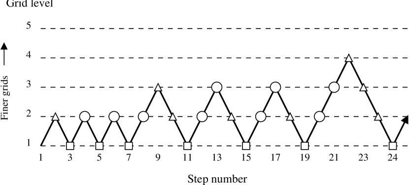
Figure 2: Schematic diagram of steps in our multigrid solver. Ascending line segments indicate prolongation, and descending line segments indicate restriction. Squares indicate direct solution on the coarsest level, triangles indicate computation of the residual, and circles indicate correction of the residual.

Our multigrid scheme uses an ascending V-cycle (Figure 2). We begin with a guess for the solution on the coarsest grid. We first apply a few Jacobi iterations to the guess (this smooths the error modes with wavelengths which are short relative to the grid spacing), then ‘prolongate’ this approximate solution to the next finer level. Our prolongation operator is simple trilinear interpolation using cell-averaged quantities with nonuniform (though nested) grids. After performing a few Jacobi iterations at this level, we then calculate the ‘residual’, the difference between the guess and the result of applying the Laplacian operator to the density on this grid. Since the Poisson equation is linear, the solution to the residual equation is just the correction which must be added to the original guess to obtain the true solution. However, since long-wavelength error modes are responsible for the Jacobi method’s slow convergence, the residual on the second level will be dominated by errors that have long wavelengths relative to this grid and shorter wavelengths relative to the coarsest grid. To remove these errors, then, we ‘restrict’ the residual back to the coarsest grid and there solve exactly for the correction (actually several Jacobi iterations on this level are sufficient). Since we are using finite volumes, restriction is equivalent to simple averaging over the fine-grid zones which lie within a given coarse-grid zone. After solving on the coarsest grid for the correction, we prolongate the correction back to the second level and apply it to the solution guess on this level. We repeat this V-cycle twice, then prolongate the solution guess to the next finer level, where we perform three more V-cycles, each time restricting all the way back to the coarsest level. We repeat this process until we reach the finest level (the original grid).

Boundary zones for the multigrid solver must be maintained both on the sides and at the corners of the computational cube for each level of the grid hierarchy, although the corners are only used for prolongations. The grid levels are nested, so their external boundaries coincide, and Dirichlet, Neumann, or periodic boundaries are simple to implement. The primary complication lies in distinguishing between cell-averaged values and cell-wall-averaged values of the potential and the density; the cell averages in the ghost zones must be chosen so as to make the cell-wall averages of the potential on the boundary possess the desired properties. We do this by writing the potential as a Taylor series about the boundary location in the direction perpendicular to the boundary, then average the series over nearby cells, obtaining a set of equations for the cell-wall averages of the potential and its derivatives in terms of the (known and unknown) interior and ghost-zone cell-averaged potential. We invert these equations (up to some limiting order) to obtain the unknown ghost-zone cell average(s) in terms of the known boundary values and interior-zone cell averages.

Isolated boundaries are boundaries outside of which the source function is identically zero. Implementing them requires that we specify the value of the potential on the boundary surface. In order to solve for the gravitational potential of isolated matter, we use a variant of James’ (1977) method. We first calculate the potential assuming Dirichlet boundaries. We then find the image distribution required to make the potential identically zero outside the boundary by evaluating the Laplacian of this Dirichlet solution on the boundary. Finally, we calculate the isolated potential of the (hollow) image distribution by computing its moments up to some maximum multipole and solving with boundary values appropriate to the corresponding multipole expansion of the potential. By subtracting this from the Dirichlet solution we obtain the desired isolated potential. We reduce the number of multipole moments required by first finding the center of mass of the image distribution and then performing the multipole expansion about this point. Our method is somewhat similar to that of Müller & Steinmetz (1995), who use a spherical-harmonic expansion of the original source function about the center of a spherically symmetric grid to compute the potential at each of the interior grid points.

3.3 Dark matter

To handle collisionless components, such as dark matter and stars, we use an $N$-body code based on the particle-mesh (PM) method (Efstathiou et al. 1985; Hockney & Eastwood 1988). This technique speeds force calculations for particles by converting particle positions to densities on a grid, then solving the Poisson equation on the grid using a fast direct or multigrid solver, and finally interpolating the potential from the grid to obtain forces at the particle locations. Since we already need to solve the Poisson equation on a grid for our hydrodynamical code, the particle-mesh method is ideally suited for integration with this code. We simply add the equivalent densities for the particles to the grid densities for the gas, then solve the Poisson equation as usual. In our case, grid densities for the particles are computed using the cloud-in-cell (CIC) operator. We also use this operator to compute interpolated forces.

Other $N$-body methods, including particle-particle-particle-mesh (P³M) and the tree methods, are often used to follow the dark matter in cluster simulations. The P³M method (Efstathiou & Eastwood 1981) extends the resolution of particle-mesh by using direct summation for the force between particles lying within a single zone. Tree methods (Hernquist 1987), on the other hand, approximate the force due to distant groups of particles using their low-order multipole moments. However, because we are using a grid-based hydrodynamical method, we do not expect to resolve features smaller than a single zone. Therefore the considerable execution time expended in the direct summation part (which scales as the square of the number of particles) of P³M would be wasted. The extra resolution provided by tree codes would likewise be wasted. Particle-mesh has another advantage for us over tree methods in the ease with which it can be integrated with the gas code.

The main difference between the PM part of COSMOS and the ‘classic’ PM codes (e. g., Efstathiou et al. 1985) is our use of a variable timestep. In order to keep the computation accurate to second order, we need a more complicated version of the standard leapfrog update of position and velocity which makes use of the gravitational acceleration on each particle stored from the preceding timestep. The resulting update steps (given here only for the $x$ component of position and velocity) are

$$x_{n+1}=x_{n}+v_{n+1/2}\Delta t_{n}$$ (33)

for the position and

$$v_{n+1/2} = v_{n-1/2}\left[1-{A_{n}\over 2}\Delta t_{n}+{1\over 3!}\Delta t_{n}^{2}\left(A_{n}^{2}-\dot{A}_{n}\right)\right]\left[1-\Delta t_{n-1}{A_{n}\over 2}+\Delta t_{n-1}^{2}{A_{n}^{2}+2\dot{A}_{n}\over 12}\right]$$ (34)

$$-\nabla\phi_{n}\left[{\Delta t_{n-1}\over 2}+{\Delta t_{n}^{2}\over 6\Delta t_{n-1}}+{\Delta t_{n-1}\over 3}-{A_{n}\Delta t_{n}\over 6}\left(\Delta t_{n}+\Delta t_{n-1}\right)\right]$$

$$-\nabla\phi_{n-1}\left[{\Delta t_{n-1}^{2}-\Delta t_{n}^{2}\over 6\Delta t_{n-1}}-{A_{n}\Delta t_{n-1}\over 12}(\Delta t_{n}+\Delta t_{n-1})\right]$$

for the velocity. Here we define $A\equiv-2\dot{a}/a$. For the first half-timestep we use a first-order accurate expression to obtain $v_{1/2}$ from the initial conditions. Note that the derivatives of the potential from the previous timestep (here denoted $\nabla\phi_{n-1}$) must be retained. This is also necessary in the PPM code in order to make second-order accurate gravitational corrections to the Riemann solver, as described by Bryan et al. (1995).

4 Code tests

As with any scientific code of this complexity it is necessary to apply COSMOS to a number of test problems with known solutions before using it on research problems. This is important not simply for the purpose of verifying that the code works as it should, but also because it gives us an intuitive understanding of the code’s strengths and weaknesses. Such an understanding is essential for making effective use of any hydrodynamical code. Accordingly, we have performed a number of tests which exercise the various code modules in different combinations. We describe the test problems and the code’s performance on each in this section.

4.1 Hydrodynamics tests

4.1.1 Sod shock-tube problem

The widely used test problem due to Sod (1978) is a Riemann shock tube problem with initial conditions specially chosen to produce all three types of fluid discontinuity (shock, contact discontinuity, and rarefaction). In this test we create two regions of constant density and pressure, separated by a plane whose normal forms specified angles with the $x$ and $y$ axes. To the left of the plane we set $\rho_{\rm L}=p_{\rm L}=1$, and to the right we set $\rho_{\rm R}=0.125$ and $p_{\rm R}=0.1$. The ratio of specific heats, $\gamma$, is 1.4, and the fluid is everywhere at rest. This test is purely hydrodynamical; no gravitational potential is used. The Sod test enables us to determine if our code satisfies the shock jump conditions and whether it correctly determines the speed of each nonlinear wave. By performing this essentially one-dimensional test in three dimensions at an angle to the grid, we can also determine how well we can resolve shocks for realistic grid sizes in 3D.

Figure 3 plots our numerical solution to the Sod problem against the analytic solution at $t=0.206$. We used a $64^{3}$ uniform grid in the box $[0,1]^{3}$; the figure shows profiles taken as a function of distance $s$ along the line segment connecting (0,0,0) and (1,1,1) (normal to the shock plane). The initial fluid discontinuity was located at $s=0.577$. In constructing the initial conditions we smoothed the discontinuity in each variable over one zone’s width to reduce the starting error resulting from the presence of all three nonlinear waves within one zone at early times. Since errors in the contact discontinuity propagate at the speed of the fluid (and hence of the discontinuity), they accumulate at the discontinuity, and any starting error will therefore be present at all later times. Even with the initial smoothing a 2% error is present in the density in the three zones in front of the contact discontinuity; this results in a similar error in the specific internal energy. Apart from this error and a slight underestimation of the slopes in the leftward-moving rarefaction wave, the numerical solution is nearly exact. The position of each of the three discontinuities is correct, and the shock and contact discontinuity are each resolved using about two zones, despite the fact that the shock is moving at an angle to the grid. This excellent shock handling is one of the primary reasons for using PPM.

4.1.2 Sedov explosion problem

To determine how well our hydrodynamical code respects the $90^{\circ}$ rotational symmetry of our grid, and to determine whether this behavior carries over to a nonuniform grid, we studied the expansion of a strong spherical shock wave into a uniform medium. In this problem, which is again purely hydrodynamical, we deposit a quantity of energy $E=1$ into a small sphere of radius $\delta r$ at the center of the grid. The pressure inside this volume, $p_{0}^{\prime}$, is given by

$$p_{0}^{\prime}={3(\gamma-1)E\over 4\pi\,\delta r^{3}}\ ,$$ (35)

where for this problem we use $\gamma=7/5$. Everywhere the density is set equal to $\rho_{0}=1$, and everywhere but the center of the grid the pressure is set to a small value, $p_{0}=10^{-5}$. The fluid is initially at rest. Sedov (1959) first obtained a self-similar analytic solution to this problem. A spherically symmetric shock wave develops; the density, pressure, and radial velocity are all functions of

$$\xi\equiv{r\over R(t)}={r\over C}\left({\rho_{0}\over Et^{2}}\right)^{1/5}\ ,$$ (36)

where $C$ is a numerical constant depending only on $\gamma$. Just behind the shock front at $\xi=1$ we have

$$\rho= \rho_{1}\equiv {\gamma+1\over\gamma-1}\rho_{0}$$

$$p= p_{1}\equiv {2\over\gamma+1}\rho_{0}u^{2}$$ (37)

$$v= v_{1}\equiv {2\over\gamma+1}u\ ,$$

where $u\equiv dR/dt$ is the speed of the shock wave. Near the center of the grid,

$$\rho(\xi)/\rho_{1} \propto \xi^{3/(\gamma-1)}$$

$$p(\xi)/p_{1} = {\rm constant}$$ (38)

$$v(\xi)/v_{1} \propto \xi\ .$$

In Figure 4 we plot the analytic solution at $t=0.0508$ against the angle average of the numerical solution found by COSMOS using a uniform $64^{3}$ grid in the box $[0,1]^{3}$. At this time the shock front is located at $r=0.314$. Since the grid is Cartesian, in the initial conditions we have attempted to minimize geometrical effects due to the shape of the grid by using an initial sphere of radius ($\delta r$) 3.5 zones. For each zone containing part of this sphere we weight the initial pressure according to the fraction of the zone which lies within the sphere using Monte Carlo averaging. Despite these efforts some small errors of geometrical origin are still present, particularly in the velocity field, where some oscillation ($\sim 7\%$) can be seen behind the shock. The position of the shock itself is accurate to 1–2 zones, which is also the width of the shock in the numerical solution. However, because the shock is narrower than one zone in the analytic solution, the density and pressure in the numerial solution do not reach their maximum analytic values $\rho_{1}$ and $p_{1}$. The density is also slightly underestimated near $r=0.25$, as is the central pressure. Given the use of a uniform, relatively coarse Cartesian grid for this spherically symmetric problem, the position and shape of the shock are well-determined.

To determine the effect of a nonuniform grid on our Sedov solution, we solved the same problem on grids with different degrees of nonuniformity. (The grid in question is static, not an adaptive grid designed to track the explosion more accurately.) In these runs the $x$-axis is nonuniform, and the $y$ and $z$ axes are uniform. Along the $x$-axis the innermost $N_{\rm inner}$ zones are uniform with spacing $\Delta$. Outside this region the zones increase in width by $\eta$ per zone toward the outer edges. Each axis uses 64 zones; the $y$ and $z$ axes each enclose the range $[0,1]$, and for the $x$-axis we fix $N_{\rm inner}$ at 16 and $\Delta$ at 1/64, allowing $\eta$ to take on several values between 0 and 20%. (Hence the box size in $x$ also varies.) For each run the explosion is thus allowed to develop up to a certain point within the same uniformly gridded region; thereafter part of the shock front expands into a region of nonuniform gridding.

Figure 5 shows, as a function of radius, the percentage change in the angle-averaged density at $t=0.0508$ for several values of $\eta$ up to 20%. Each density profile has been interpolated to the same uniform grid. Because the shock is only partly resolved even on the uniform grid at $t=0.0508$, the increased zone width for large $\eta$ forces the shock to be substantially broadened, leading to an overestimate of the density ahead of the shock and an underestimate behind it. The average density is also underestimated by a constant 1–2% well behind the shock for $\eta\geq 10\%$ because the broadened shock does not sufficiently compress the ambient medium. For $\eta=5\%$ the magnitude of these effects is much smaller.

As the explosion proceeds in the analytic solution, the width of the shock front increases, and its amplitude decreases. If the zone size increases much faster than the rate of increase of the width of the shock, the numerical solution will continue to degrade as the shock propagates outward. For this problem the value of $\eta$ at which the zone size begins to increase faster than the shock width appears to lie between 5% and 10%. In general, the amount of nonuniformity to use must be balanced against the need to resolve fine flow structures near the edge of the grid. If the zone size is permitted to be too large, the zone-averaged density, pressure, and velocity may be correct, but the position and size of flow structures will be poorly determined, and their dynamical effects (such as heating and compression) on the surrounding gas will also be in error.

4.1.3 Jeans instability problem

Using the Jeans instability we verified that the gas dynamical terms involving the gravitational potential are correctly implemented in COSMOS. To do this we studied the dispersion relation of stable perturbations to a uniform, self-gravitating medium. The initial conditions for this problem, which we solved in two dimensions with periodic boundaries, are, at time $t=t_{i}$,

$$\rho(x,y,t_{i}) = \rho_{0}\left[{1+\delta\cos(\kappa x)\cos(\kappa y)}\right]$$

$$p(x,y,t_{i}) = p_{0}\left[{1+\gamma\delta\cos(\kappa x)\cos(\kappa y)}\right]$$

$$v_{x}(x,y,t_{i}) = {\delta|\omega|\over\sqrt{2}\kappa}\left[{\sin(\kappa x)\cos(\kappa y)\over 1-\delta\cos(\kappa x)\cos(\kappa y)}\right]$$ (39)

$$v_{y}(x,y,t_{i}) = {\delta|\omega|\over\sqrt{2}\kappa}\left[{\cos(\kappa x)\sin(\kappa y)\over 1-\delta\cos(\kappa x)\cos(\kappa y)}\right]\ ,$$

where the perturbation amplitude $\delta\ll 1$, and where $\omega$ is defined as follows. The stability of the perturbation is determined by the relationship between the wavenumber $k=\sqrt{2}\kappa$ and the Jeans wavenumber $k_{J}$ (Chandrasekhar 1961), where $k_{J}$ is given by

$$k_{J}\equiv{\sqrt{4\pi G\rho_{0}}\over c_{0}}\ ,$$ (40)

and where $c_{0}$ is the sound speed:

$$c_{0}=\sqrt{\gamma p_{0}\over\rho_{0}}\ .$$ (41)

If $k>k_{J}$, the perturbation is stable and oscillates with frequency

$$\omega=\sqrt{c_{0}^{2}k^{2}-4\pi G\rho_{0}}\ ;$$ (42)

otherwise it grows exponentially, with a characteristic timescale given by $\tau=(i\omega)^{-1}$.

We checked the dispersion relation (42) for stable perturbations with $\gamma=5/3$ by fixing $\rho_{0}$ and $p_{0}$ and performing several runs with different $k$. We followed each case for roughly ten oscillation periods using a uniform $64^{2}$ grid in the box $[0,\sqrt{\pi\gamma}/2]^{2}$ with units in which $\rho_{0}=p_{0}=G=1$. (The box size is chosen so that $k_{J}$ is smaller than the smallest nonzero wavenumber which can be resolved on the grid. This prevents numerical errors at wavenumbers less than $k_{J}$ from being amplified by the physical Jeans instability.) We then computed the oscillation frequency in each case by measuring the time interval required for the density at the center of the grid to undergo exactly ten oscillations. The resulting dispersion relation is compared to equation (42) in Figure 6. It can be seen from this plot that our code correctly reproduces equation (42). At the highest wavenumber ($k=62.132$), each oscillation is resolved using only about 9 cells, and the average timestep (which depends on $c_{0}$, $\Delta x$, and $\Delta y$, and has nothing to do with $k$) turns out to be about one-fifth of an oscillation. Hence the frequency determined from the numerical solution for this value of $k$ is somewhat more poorly determined than for the other runs. Overall, however, the frequencies are correct to about 1%.

4.1.4 Zel’dovich pancake

The cosmological pancake problem (Zel’dovich 1970) provides a good simultaneous test of the self-gravity and cosmological expansion code. Analytic solutions well into the nonlinear regime are available for both $N$-body and hydrodynamical codes (Anninos & Norman 1994), permitting an assessment of the code’s accuracy. After caustic formation the problem provides a stringent test of the code’s ability to track thin, poorly resolved features and strong shocks using most of the basic physics needed for cosmological problems. Also, as pancakes represent single-mode density perturbations, coding this test problem is useful as a basis for creating more complex initial conditions.

We set the initial conditions for the pancake problem in the linear regime using the analytic solution given by Anninos and Norman (1994). In a universe with $\Omega_{0}=1$ at redshift $z$, a perturbation of wavenumber $k$ which collapses to a caustic at redshift $z_{c}<z$ has comoving density and velocity given by

$$\rho(x_{e};z) = \bar{\rho}\left[1+{1+z_{c}\over 1+z}\cos\left(kx_{\ell}\right)\right]^{-1}$$ (43)

$$v(x_{e};z) = -H_{0}(1+z)^{1/2}(1+z_{c}){\sin kx_{\ell}\over kx_{\ell}}\ ,$$

where $\bar{\rho}$ is the comoving mean density. Here $x_{e}$ is the distance of a point from the pancake midplane, and $x_{\ell}$ is the corresponding Lagrangian coordinate, found by iteratively solving

$$x_{e}=x_{\ell}-{1+z_{c}\over 1+z}{\sin kx_{\ell}\over k}\ .$$ (44)

The temperature solution is determined from the density under the assumption that the gas is adiabatic with ratio of specific heats $\gamma$:

$$T(x_{e};z)=(1+z)^{2}\bar{T}_{\rm fid}\left[\left({1+z_{\rm fid}\over 1+z}\right)^{3}{\rho(x_{e};z_{\rm fid})\over\rho(x_{e};z)}\right]^{\gamma-1}\ .$$ (45)

The mean temperature $\bar{T}_{\rm fid}$ is specified at a redshift $z_{\rm fid}$.

At caustic formation ($z=z_{c}$), planar shock waves form on either side of the pancake midplane and begin to propagate outward. A small region at the midplane is left unshocked. Immediately behind the shocks, the comoving density and temperature vary approximately as

$$\rho(x_{e};z) \approx \bar{\rho}{18\over\left(kx_{\ell}\right)^{2}}{\left(1+z_{c}\right)^{3}\over\left(1+z\right)^{3}}$$ (46)

$$T(x_{e};z) \approx {\mu H_{0}^{2}\over 6k_{B}k^{2}}\left(1+z_{c}\right)\left(1+z\right)^{2}\left(kx_{\ell}\right)^{2}\ .$$

At the midplane, which undergoes adiabatic compression, the comoving density and temperature are approximately

$$\rho_{\rm center} \approx \bar{\rho}\left[{1+z_{\rm fid}\over 1+z}\right]^{3}\left[{3H_{0}^{2}\mu\over k_{B}\bar{T}_{\rm fid}k^{2}}{\left(1+z_{c}\right)^{4}\left(1+z\right)^{3}\over 1+z_{\rm fid}}\right]^{1/\gamma}$$ (47)

$$T_{\rm center} \approx {3H_{0}^{2}\mu\over k_{B}k^{2}}\left(1+z\right)^{2}\left(1+z_{c}\right)^{4}{\bar{\rho}\over\rho_{\rm center}}\ .$$

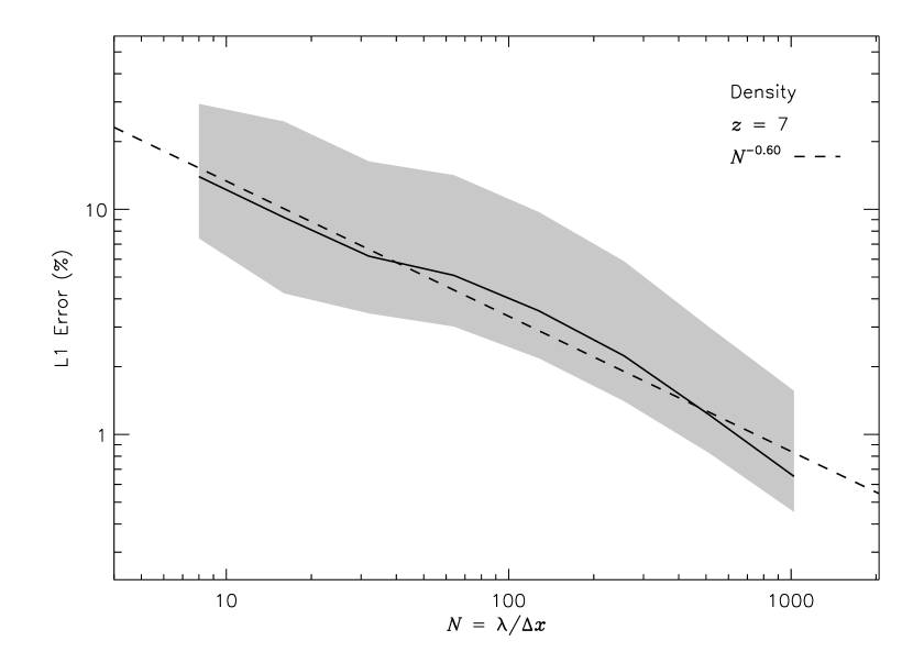
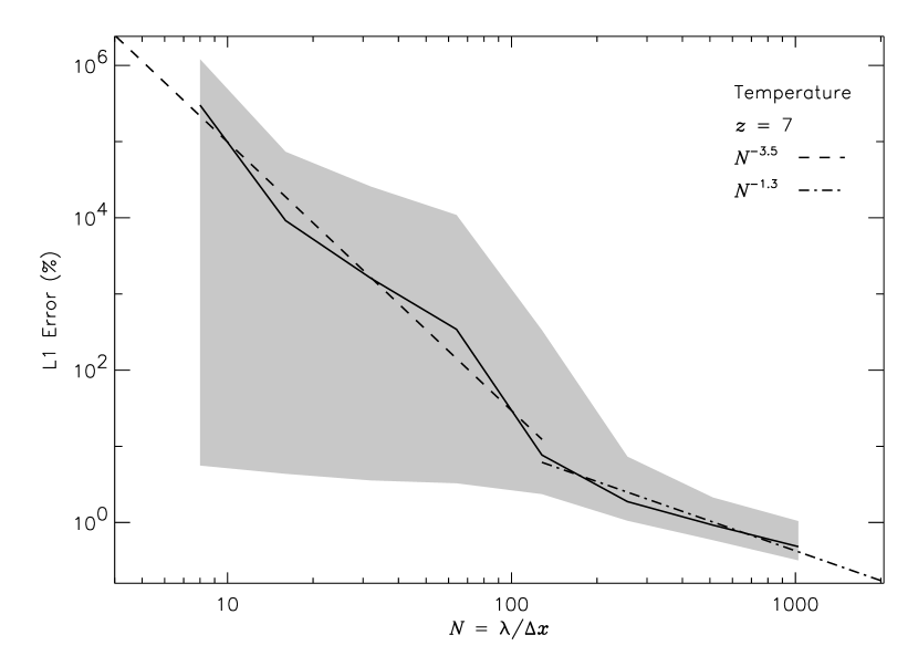
Figure 7: One-dimensional convergence results for the gas-only Zel’dovich pancake problem, as functions of the number of zones $N$, for fixed perturbation wavelength $\lambda$. Solid lines indicate the L1 error norm (eq. [50]), while shaded areas indicate RMS deviations of the error from the L1 norm. Dashed lines indicate power-law relations for comparison.

To test the convergence of the code, we performed several different one-dimensional pancake test runs with fixed perturbation wavelength and caustic redshift and varying spatial resolution. Each run used $k=2\pi/(10{\rm\ Mpc})$, $z_{c}=5$, and an initial redshift $z_{i}=50$. In each run we also fixed $z_{\rm fid}=200$, $\bar{T}_{\rm fid}=550$ K, $\gamma=5/3$, $\Omega_{0}=1$, and $H_{0}=50$ km s^-1 Mpc^-1. We assumed a 75% H/25% He composition for the purpose of computing the pressure using the temperature. Using the analytic solution (eqs. [43] – [45]), we computed L1 error norms for density and temperature in each run at $z\approx 7$, in the mildly nonlinear phase of the collapse. We define the L1 error norm as in equation (50) below. The results appear in Figure 7. The density converges slowly, with the error varying approximately as $\Delta x^{0.6}$. The temperature converges more rapidly, with the error varying as $\Delta x^{3.5}$ for $\Delta x>\lambda/128$ and then as $\Delta x^{1.3}$ for smaller $\Delta x$. The roughly linear asymptotic convergence for the temperature is consistent with other work, for example that of Bryan et al. (1995), but the density convergence rate is somewhat slower. Nevertheless, the absolute error of a few percent for $\Delta x\sim\lambda/100$—$\lambda/200$ is consistent with their results for both variables.

To examine the performance of COSMOS on this problem in multidimensions, we performed a run with the same initial conditions using a doubly periodic $256^{2}$ grid. The pancake midplane was inclined $45^{\circ}$ to the $x$ axis, and the zone spacing was chosen so that two wavelengths fit into the box diagonal. In Figure 8 the results of this run are compared to the 256-zone 1D solution at three different redshifts corresponding to the mildly nonlinear regime ($z=7.4$), the time immediately following caustic formation ($z=4.4$), and a time well into the nonlinear, post-caustic evolution ($z=0$). The profiles for the $256^{2}$ run are derived by interpolating along the grid diagonal. In this run only 128 zones fit within a perturbation wavelength, so the spatial resolution is one-half that of the 1D 256-zone run. With the exception of the innermost 1–2 zones, the 2D results are typically within a few percent of the 1D results. Differences of note include a 20% underdensity in the 2D case at $z=7.4$ and a significant overestimate in the central temperature at $z=4.4$. In the latter case the caustic is unresolved by the mesh, and only the innermost zone is hot. The velocity in the innermost zone is different by as much as a factor of two at all three redshifts.

4.2 Tests of the Poisson solver

4.2.1 Miyamoto-Nagai potential

We tested the potential solver with isolated boundaries using the Miyamoto-Nagai potential (Miyamoto & Nagai 1975). This is an axisymmetric, flattened potential designed to mimic the light distribution of a disk galaxy. It is given in cylindrical coordinates by

$$\phi_{\rm MN}(r,z)\equiv-{GM\over\sqrt{r^{2}+\left(a+\sqrt{z^{2}+b^{2}}\right)^{2}}}\ ,$$ (48)

where $M$ is the total mass, and the ratio of the axis parameters $b/a$ determines how flattened the potential is. As $b/a\longrightarrow 0$, $\phi_{\rm MN}$ tends toward the Kuzmin disk potential, and as $b/a\longrightarrow\infty$, $\phi_{\rm MN}$ tends toward the spherically symmetric Plummer potential. Thus for different $b/a$ values $\phi_{\rm MN}$ contains different contributions from high-order multipole moments, making this a good test of our moment-based isolated boundary solver. The density function corresponding to this potential is straightforward to derive using the Poisson equation; it is

$$\rho_{\rm MN}(r,z)=\left({b^{2}M\over 4\pi}\right){ar^{2}+\left(a+3\sqrt{z^{2}+b^{2}}\right)\left(a+\sqrt{z^{2}+b^{2}}\right)^{2}\over\left[r^{2}+\left(a+\sqrt{z^{2}+b^{2}}\right)^{2}\right]^{5/2}\left(z^{2}+b^{2}\right)^{3/2}}\ .$$ (49)

Using this density function we computed Miyamoto-Nagai potentials with the isolated Poisson solver in COSMOS for $b/a=0.1$, $1$, and $10$ using a $128^{2}\times 64$ grid in boxes containing 98–99% of the total mass. The innermost one-half of the zones in each dimension were uniform, and the remainder increased in width by 5% per zone toward the outside edges. We used units in which $G=M=a=1$.

In our treatment of isolated boundaries we compute boundary values for the image potential using a truncated multipole expansion of the image mass distribution. To verify that this expansion was implemented correctly, we performed runs with four different values of $\ell_{\rm max}$, the largest multipole moment. In Figure 9 we plot average errors for our computed potentials as a function of $\ell_{\rm max}$ for our three values of $b/a$. We define the error $E(\ell_{\rm max},b/a)$ as

$$E(\ell_{\rm max},b/a)\equiv{100\over V}\sum_{ijk}\left|{\phi_{ijk}-\phi_{{\rm MN},ijk}\over\phi_{{\rm MN},ijk}}\right|\Delta V_{ijk}\ ,$$ (50)

where the sum is taken over all of the cells in the grid, and the total volume $V$ of the grid is the sum of cell volumes $\Delta V_{ijk}$. Figure 9 shows that including only the first three multipole terms already gives a fairly good estimate of the potential; the maximum percentage error in any cell for $\ell_{\rm max}=2$ is between 6.5% and 7.5%, and the plotted averages range from 2.2% to 2.7%. Increasing the value of $\ell_{\rm max}$ brings the average and maximum errors down substantially, showing that the isolated boundary solver is including higher-order moments properly. The curves begin to level off at values less than 1% above $\ell_{\rm max}=10$; this level of error is consistent with the amount of mass which lay outside the grid and hence was excluded from each calculation. The maximum error at $\ell_{\rm max}=14$ is about 1.5% in all three cases.

For other problems the multipole content of the density field may differ, so these test results do not show that 1% errors will be achieved with $\ell_{\rm max}\approx 10$ for any arbitrarily chosen density field. However, this will be true even for quite flattened density fields. Errors caused by underestimating $\ell_{\rm max}$ will be largest near the boundaries of the grid as long as most of the mass is near the center.

4.2.2 Particle-mesh force resolution test

Because of the particle-mesh force-smoothing procedure, dark matter particles experience an effective potential that deviates from the Newtonian $1/r$ dependence at small interparticle separations $r$. This deviation is greatest on length scales less than or comparable to the zone spacing $\Delta r$. In addition, the introduction of a grid breaks the rotational symmetry of the equations of motion, so interparticle forces are not isotropic for $r\mathrel{<\kern-10.00002pt\lower 3.87495pt\hbox{$\sim$}}\Delta r$. When performing simulations in which small-scale structure (relative to the grid in use) appears, it is important to have an estimate of the magnitude of these errors and the value of $r/\Delta r$ at which they become important.

To quantify these effects, we performed a test in which we chose 10,000 randomly placed pairs of particles on a $32^{3}$ grid, computed forces for each pair using the multigrid solver and particle-mesh code from COSMOS, and tabulated the resulting forces as functions of the particle positions. The first particle in each pair was chosen to lie within one zone of the center of the grid, while the second particle was chosen to lie between 0.1 and 10 zones from the first, with a random position angle relative to the first. In this test each particle had unit mass, and the value of $G$ was unity. For the $i$th particle of the $j$th pair we computed radial ($f_{ij,r}$) and azimuthal ($f_{ij,\theta}$) force components relative to the line connecting the particle to its partner; then for the pair we computed the average of the magnitudes of the radial and the azimuthal components for the two particles:

$$\bar{f}_{j,X}\equiv{1\over 2}\left(\left|f_{1j,X}\right|+\left|f_{2j,X}\right|\right)$$ (51)

where $X=r,\theta$. We collected the particle pairs in radial bins of logarithmic width 0.05, then computed mean and RMS deviations for the binned forces.

In Figure 10 we show the results as functions of radius. Overall the results are comparable to those obtained by Efstathiou et al. (1985): our effective particle force resolution is about two zones. For $r=\Delta r$ the mean radial force is 50% of the expected value, and the force anisotropy (ratio of mean azimuthal to mean radial force) is about 13%. For particle separations smaller than this, the mean radial force is proportional to $r$, and the force anisotropy is roughly constant at around 7%. As $r\rightarrow\infty$ the azimuthal force drops as $r^{-3}$, so the force anisotropy drops approximately as $r^{-1}$. At $r\approx 9$ the azimuthal force turns upward slightly; this illustrates the effect of placing the second particle of some pairs within 4–5 zones of the grid boundary. We discuss this effect in more detail below.

For particle separations less than one zone, the RMS deviations in the radial and azimuthal force components are each roughly constant at 20% and 5%, respectively, of the mean radial force. For $r>2\Delta r$ the radial RMS deviation drops to about 7% of the radial mean, while the azimuthal RMS deviation decreases almost as fast as the mean azimuthal force, becoming less than 0.2% of the radial mean at $r=10\Delta r$. The azimuthal RMS deviation also shows a slight upturn for particles close to the boundary.

The deviations from a $1/r^{2}$ force law at large $r$ result from a self-force felt only by particles close to the edge of the grid. As Hockney and Eastwood (1988) show, self-forces arise in PM schemes when either the density assignment and force interpolation operators differ or the effective Green’s function ${\bf G}_{ijklmn}$ fails to satisfy the criterion

$${\bf G}_{ijklmn}=-{\bf G}_{lmnijk}\ .$$ (52)

The effective Green’s function is related to the zone-averaged gravitational field ${\bf g}_{ijk}$ by

$${\bf g}_{ijk}=\sum_{lmn}{\bf G}_{ijklmn}\rho^{\rm PM}_{lmn}\Delta V_{lmn}\ ,$$ (53)

where $\rho^{\rm PM}_{lmn}$ is the density assigned to the grid by the particle-mesh scheme, $\Delta V_{lmn}$ is the volume of a single grid zone, and the sum is taken over all zones. Because we use the CIC operator both to assign densities to the grid and to interpolate forces to particle positions, any self-forces are due to errors in the potential which cause ${\bf G}$ to violate equation (52). In our case, errors in ${\bf G}$ arise because we use a finite multipole expansion to obtain boundary conditions for isolated problems.

We have examined this effect by performing another test in which one particle is placed at the center of the grid and the second particle is placed at increasing distances from the center along one coordinate axis. By varying the grid size, we can use this test to determine how close to the edge of the grid a particle can be before it experiences a significant self-force. For this test we use $\ell_{\rm max}=10$ in the multigrid solver. Figure 11 compares the results on grids with $16^{3}$, $32^{3}$, and $64^{3}$ zones. In each case the force on the second particle begins to deviate from the expected value when the second particle is about five zones from the edge of the grid.

Note that the two-particle potential is more susceptible to this effect than the Miyamoto-Nagai test potential because of the relative importance in this case of mass close to the edge of the grid. The effect is important only for small numbers of particles close to the edge of the grid; it is not important for particles near the boundary orbiting in the potential of a large group of particles near the center, and it is not present when periodic boundary conditions are used.

4.3 $N$-body tests

4.3.1 Time integration accuracy

To account for the varying timestep size, COSMOS implements equation (34) to update the dark matter positions and velocities. To test this algorithm, we set up two particles in a simple circular orbit and monitored the accuracy of the orbit as we varied the timestep $\Delta t$ and the zone size $\Delta x$. In addition to testing the algorithm, this problem enables us to determine the regions in $(\Delta x,\Delta t)$ space that are appropriate for larger, more interesting problems.

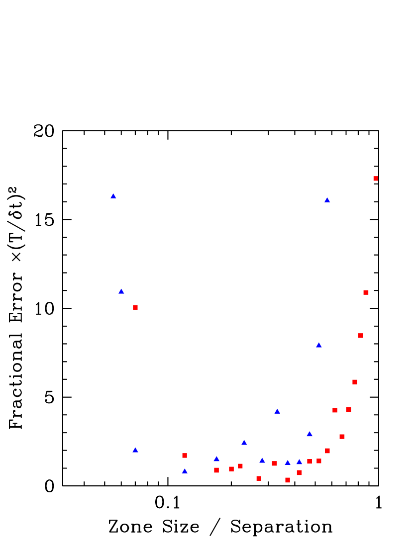
Figure 12: RMS error in the circular orbit of two particles as a function of the ratio of the zone spacing $\Delta x$ to the (fixed) interparticle separation $r$. Choices of timestep $\Delta t$ corresponding to 0.015 orbital period (triangles) and 0.046 orbital period (squares) are shown.

Figure 12 shows the root mean square (RMS) error in the interparticle separation after six orbital periods as a function of $\Delta x$. For $\Delta x$ larger than the particle separation, the $1/r^{2}$ force is calculated incorrectly due to the mesh smoothing. The problem of resolving forces on scales smaller than a zone size is a well-known one; Figure 12 simply points out that our force resolution is roughly one or two zones. For very small $\Delta x$, on the other hand, each particle traverses more than one zone in a single timestep, which again leads to large errors. To alleviate this second problem, in production runs we choose $\Delta t$ with the requirement that no dark matter particle travel more than a fraction $\sigma_{\rm dm}$ of a zone during a single timestep:

$$\Delta t_{\rm dm}=\sigma_{\rm dm}\min_{\rm particles}\left[{\Delta x_{i}\over v_{{\rm dm},x}^{p}},{\Delta y_{j}\over v_{{\rm dm},y}^{p}},{\Delta z_{k}\over v_{{\rm dm},z}^{p}}\right]\ ,$$ (54)

where $(i,j,k)$ are the indices of the zone containing the $p$th particle. Figure 12 shows that setting this fraction equal to one is an acceptable choice. The two groups of points in this plot correspond to different ratios of the timestep to the orbital period. If we denote this ratio by $f$, then we require

$${\Delta x\over 2r}>{\pi f\over\sigma}$$ (55)

for accuracy. The squares indicate runs with $f=0.046$, and the triangles indicate runs with $f=0.015$. If we choose $\sigma_{\rm dm}=1$, then the two groups of runs require $\Delta x/2r>0.14$ and $0.047$ respectively. For the first group, runs with $\Delta x/2r>0.1$ are observed to be relatively accurate, while for the second group, the error is low for $\Delta x/2r>0.06$. In the regime where the zone size is not too big or too small relative to the timestep, we see that the cumulative error does indeed scale as $\Delta t^{2}$: the algorithm of equation (34) is accurate to second order.

4.3.2 Spherical collapse problem

A well-known cosmological problem with an analytic solution is the case of a spherical overdensity (e. g., Padmanabhan 1993). The solution to this problem is best described in terms of the radius $R(t)$ which encloses a mass $M$ at time $t$:

$$R(t;M)=R(t_{i};M)\sin^{2}\left[{\theta\over 2}\right]{1+\delta_{i}\over\delta_{i}}\ .$$ (56)

Here $t_{i}$ and $\delta_{i}$ denote the time and fractional overdensity at which the simulation starts. The parameter $\theta$ is a timelike parameter; in a flat, matter-dominated universe, the redshift can be expressed in terms of $\theta$ as

$$1+z=(1+z_{i})\left[1+{3\over 4}{1+\delta_{i}\over\delta_{i}^{3/2}}\bigg{(}\theta-\sin\theta-\theta_{i}+\sin\theta_{i}\bigg{)}\right]^{-2/3}.$$ (57)

Equation (56) holds until the radius reaches a maximum value at $\theta=\pi$, after which time virialization occurs.

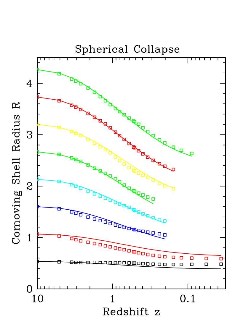
Figure 13: Time evolution of the radius of different mass shells in the dark-matter-only spherical collapse test. Units are such that the zone spacing is unity. Points are results from a $32^{3}$ simulation; solid lines are the analytic solution, plotted until the time of maximum physical radius.

On a $32^{3}$ grid with $32^{3}$ particles we set up spherically symmetric initial conditions. In units in which the cell size is unity, within a radius of five units from the center of the grid we constructed a uniform overdensity with $\delta_{i}=0.3$. In an annulus ranging from $r=5$ to $r=8$ we placed an underdensity so that the average density within $r=8$ was equal to the background density. Figure 13 shows the time evolution of several (comoving) radii, compared with the analytic result of equation (56). The larger shells track the analytic solution well, verifying that all factors of $a(t)$ are correctly implemented in the dark matter code. As expected, the small shells do worse: the force on these shells comes predominantly from particles concentrated at a distance of one to two zones. The deviations from equation (56) for these shells are consistent with the underestimate of the gravitational force introduced by the particle-mesh smoothing at this distance.

4.3.3 One-dimensional Plane Wave

The Zel’dovich pancake (Section 4.1.4) also serves as a test of the $N$-body code. To initialize this problem, we place particles at the zone centers of a $16^{3}$-zone grid, then perturb their positions slightly in the $x$-direction by amounts

$$\delta x_{i}\propto\cos(2\pi kx_{i}/L)$$ (58)

with $x_{i}$ the unperturbed positions and $k$ an integer. Small-scale perturbations correspond to large $k$. We consider only perturbations which vary on scales larger than a zone width, ie. those with $k<<N_{x}$. If the particles’ peculiar velocities $\delta v_{x,i}$ are also proportional to $\cos(2\pi kx_{i}/L)$, then in the linear regime (assuming a flat universe) both $\delta x_{i}$ and $\delta v_{x,i}$ should grow with time as the scale factor $a(t)$.

To determine how accurately their code could follow such perturbations, Efstathiou et al. (1985) tabulated the RMS deviation of position and velocity from the analytic solution for particles on a $16^{3}$ mesh. Since we solve Poisson’s equation differently than the standard PM code, it is useful to compare our results with theirs. Figure 14 shows the RMS errors in position and velocity for linear perturbations with several different values of the wavenumber $k$. The multigrid solver and variable-timestep integrator used in COSMOS produce results quite similar to (but slightly better than) the FFT/fixed-timestep technique used by Efstathiou et al. (1985).

5 Conclusion

In this paper we have described COSMOS, a new hybrid code for solving cosmological problems involving gas and collisionless matter, including self-gravity, cosmological expansion, and radiative cooling. COSMOS solves the inviscid fluid equations using the piecewise-parabolic method on a static, nonuniform structured grid. The code treats collisionless matter using the cloud-in-cell variant of the particle-mesh method, and it computes the gravitational potential using a linear full multigrid solver. COSMOS supports both periodic boundaries, suitable for large-scale structure problems, and isolated boundaries, suitable for simulations of isolated systems. This code has already been used to study mergers between clusters of galaxies by Ricker (1998) and Ricker & Sarazin (2000).

Several new features of COSMOS distinguish it from other existing PM-PPM codes. In particular, the multigrid Poisson solver can determine the gravitational potential of isolated matter distributions and properly takes into account the finite-volume discretization required by PPM. All components of the code are constructed to work with a nonuniform mesh, preserving second-order spatial differences. The PPM code uses vacuum boundary conditions for isolated problems, preventing inflows when appropriate. The PM code uses a second-order variable-timestep time integration scheme. In this paper we have discussed the equations solved by COSMOS and described the algorithms used, with emphasis on these features. We have also reported on results from a suite of standard test problems, demonstrating that COSMOS works as expected.

In closing we note some implementation details. COSMOS is designed to run on parallel computers using the Parallel Virtual Machine (PVM) message-passing library. A version using the Message-Passing Interface (MPI) is currently under development. Also, COSMOS features a modular design which simplifies the addition of new physics and the configuration of the code for different types of problems. The modular design of COSMOS has served as the basis for FLASH, an adaptive mesh-refinement PPM code currently under development at the University of Chicago ASCI Flash Center. Details of the FLASH code design will appear in a forthcoming paper (Fryxell et al. 1999).

Figure 1: Example multigrid hierarchy for a 2D grid which is nonuniform in the $x$-direction and uses three levels of grid refinement. The thickness of the lines bounding a cell indicate its grid level; for example, the thickest lines indicate cell divisions on the coarsest level. The $x$-coordinates of cell centers on each level are indicated by numbers.

Figure 3: Density, pressure, velocity, and specific internal energy in the Sod problem at $t=0.206$. Solid lines represent the analytic solution; squares indicate numerical solution values interpolated along the line normal to the shock which passes through the origin.

Figure 4: Density, pressure, and velocity for the Sedov explosion problem on a uniform $64^{3}$ grid at $t=0.0508$. Squares represent the angle-averaged numerical solution, and solid lines represent the analytic solution.

Figure 5: Percentage deviation from the uniform-grid case of the angle-averaged solution to the Sedov explosion problem on grids of varying nonuniformity.

Figure 6: Test of the Jeans dispersion relation for gravitationally stable perturbations. Squares indicate oscillation frequencies taken from the test calculations; the solid line indicates the expected relation.

Figure 8: Comparison of the $256^{2}$ gas-only pancake test at three different redshifts with the 256-zone 1D solution. Density, temperature, and velocity amplitude are shown. Symbols represent values interpolated from the 2D calculation; lines represent values taken from the 1D calculation.

Figure 9: Average error in Miyamoto-Nagai potential calculations for different flatness ratios $b/a$, plotted as a function of the largest multipole moment $\ell_{\rm max}$ used in the computation of isolated boundaries.

Figure 10: Results of the PM force resolution test. (a) Mean binned radial (filled circles) and azimuthal (open circles) components of the interparticle force for randomly positioned particle pairs. The dashed line indicates the expected $1/r^{2}$ force. Here $r$ is expressed in units of the zone spacing $\Delta r$. (b) RMS deviations for the binned radial and azimuthal components, expressed as fractions of the mean binned radial force.

Figure 11: Results of the PM force resolution test with a single pair of particles, where the first member of each pair is placed at the center of the grid and the second member is placed at increasing distances from the center along the line connecting the center to one of the grid boundaries. The plot shows the ratio of the force on the second particle to the expected value as a function of the ratio of the particle separation $r$ to the box size $L$.

Figure 14: RMS errors in position ($\Delta x_{\rm RMS}$) and velocity ($\Delta v_{\rm RMS}$) for the dark-matter-only plane wave problem in the linear regime. Lines represent results from simulations using a $16^{3}$ grid and $16^{3}$ particles. Results for three different values of the wavenumber $k$ are shown. Points represent values from equivalent runs by Efstathiou et al. (1985), who used an FFT Poisson solver instead of the multigrid method used here.

References

- (1) Anninos, W. Y. Norman, M. L. 1994, ApJ, 429, 434
- (2) Brandt, A. 1977, Math. Comp., 31, 333
- (3) Bryan, G. L., Norman, M. L., Stone, J. M., Cen, R., Ostriker, J. P. 1995, Comp. Phys. Comm., 89, 149
- (4) Chandrasekhar, S. 1961, Hydrodynamic and Hydromagnetic Stability (Oxford: Clarendon)
- (5) Cen, R. 1992, ApJS, 78, 341
- (6) Colella, P. 1985, SIAM J. Sci. Stat. Comput., 6, 104
- (7) Colella, P. Glaz, H. M. 1985, J. Comp. Phys., 59, 264
- (8) Colella, P. Woodward, P. 1984, J. Comp. Phys., 54, 174
- (9) Couchman, H. M. P., Thomas, P. A., Pearce, F. R. 1995, ApJ, 452, 797
- (10) Douglas, C. C. 1992, SIAM News, 25, 14
- (11) Efstathiou, G., Davis, M., Frenk, C. S., & White, S. D. M. 1985, ApJS, 57, 241
- (12) Efstathiou, G. Eastwood, J. W. 1981, MNRAS, 194, 503
- (13) Evrard, A. E. 1988, MNRAS, 235, 911
- (14) Frenk, C. S. et al. 1999, ApJ, 525, 554
- (15) Fryxell, B. et al. 1999, ApJS, submitted
- (16) Gheller, C., Pantano, O., Moscardini, L. 1998, MNRAS, 295, 519
- (17) Gingold, R. A. Monaghan, J. J. 1977, MNRAS, 181, 375
- (18) Gnedin, N. Y. 1995, ApJS, 97, 231
- (19) Godunov, S. K. 1959, Mat. Sbornik, 47, 271
- (20) Hackbusch, W. 1985, Multi-Grid Methods and Applications (Berlin: Springer-Verlag)
- (21) Harten, A. 1983, J. Comp. Phys., 49, 151
- (22) Hernquist, L. 1987, ApJS, 64, 715
- (23) Hernquist, L. Katz, N. 1989, ApJS, 70, 419
- (24) Hockney, R. W. Eastwood, J. W. 1988, Computer Simulation Using Particles (Bristol: IOP)
- (25) Kang, H., Ostriker, J. P., Cen, R., Ryu, D., Hernquist, L., Evrard, A. E., Bryan, G. L., Norman, M. L. 1994, ApJ, 430, 83
- (26) Kritsuk, A., Böhringer, H., Müller, E. 1998, MNRAS, 301, 343
- (27) James, R. A. 1977, J. Comp. Phys., 25, 71
- (28) van Leer, B. 1979, J. Comp. Phys., 32, 101
- (29) Lucy, L. B. 1977, AJ, 82, 1013
- (30) Miyamoto, M. Nagai, R. 1975, PASJ, 27, 533
- (31) Müller, E. Steinmetz, M. 1995, Comp. Phys. Commun., 89, 45
- (32) Navarro, J. F. White, S. D. M. 1993, MNRAS, 265, 271
- (33) Norman, M. L. Bryan, G. L. 1999, in Numerical Astrophysics 1998, eds. S. M. Miyama, K. Tomisaka, T. Hanawa (Boston: Kluwer)
- (34) Owen, J. M., Villumsen, J. V., Shapiro, P. R., Martel, H. 1998, ApJS, 116, 155
- (35) Padmanabhan, T. 1993, Structure Formation in the Universe (Cambridge: CUP)
- (36) Peebles, P. J. E. 1993, Principles of Physical Cosmology (Princeton, NJ: Princeton Univ. Press)
- (37) Pen, U.-L. 1998, ApJS, 115, 19
- (38) Press, W. H., Teukolsky, S. A., Vetterling, W. T., Flannery, B. P. 1992, Numerical Recipes in FORTRAN, 2d ed. (Cambridge: Cambridge Univ. Press)
- (39) Quilis, V., Ibáñez, J. M., Sáez, D. 1996, ApJ, 469, 11
- (40) Quilis, V., Ibáñez, J. M., Sáez, D. 1998, ApJ, 502, 518
- (41) Ricker, P. M. 1998, ApJ, 496, 670
- (42) Ricker, P. M. Sarazin, C. L., 2000, in preparation
- (43) Roache, P. J. 1998, Fundamentals of Computational Fluid Dynamics, 2d ed. (Albuquerque: Hermosa)
- (44) Roe, P. L. 1981, J. Comp. Phys., 43, 357
- (45) Roettiger, K., Stone, J. M., Mushotzky, R. F. 1997, ApJ, 482, 588
- (46) Ryu, D., Ostriker, J. P., Kang, H., Cen, R. 1993, 414, 1
- (47) Sedov, L. I. 1959, Similarity and Dimensional Methods in Mechanics (New York: Academic)
- (48) Sod, G. 1978, J. Comp. Phys., 27, 1
- (49) Sornborger, A., Fryxell, B., Olson, K., MacNeice, P. 1996, astro-ph/9608019
- (50) Steinmetz, M. 1996, MNRAS, 278, 1005
- (51) Strang, G. 1968, SIAM J. Numer. Anal., 5, 506
- (52) Thompson, K. W. 1987, J. Comp. Phys., 68, 1
- (53) Zel’dovich, Ya. B. 1970, A&A, 5, 84