Statistics of Weak Lensing at Small Angular Scales:
Analytical Predictions for Lower Order Moments

Abstract

Weak lensing surveys are expected to provide direct measurements of the statistics of the projected dark matter distribution. Most analytical studies of weak lensing statistics have been limited to quasilinear scales as they relied on perturbative calculations. On the other hand, observational surveys are likely to probe angular scales less than 10 arcminutes, for which the relevant physical length scales are in the nonlinear regime of gravitational clustering. We use the hierarchical ansatz to compute the multi-point statistics of the weak lensing convergence for these small smoothing angles. We predict the multi-point cumulants and cumulant correlators up to fourth order and compare our results with high resolution ray tracing simulations. Averaging over a large number of simulation realizations for four different cosmological models, we find close agreement with the analytical calculations. In combination with our work on the probability distribution function, these results provide accurate analytical models for the full range of weak lensing statistics. The models allow for a detailed exploration of cosmological parameter space and of the dependence on angular scale and the redshift distribution of source galaxies. We compute the dependence of the higher moments of the convergence on the parameters $\Omega$ and $\Lambda$ and on the nature of gravitational clustering.

1 Introduction

Weak distortions in the images of high redshift galaxies due to gravitational lensing provide us with valuable information about the mass distribution in the universe. The study of such distortions provides us a unique way to probe the statistical properties of the intervening large-scale structure. Traditionally, the study of gravitational clustering in the quasi-linear and non-linear regimes has been done by analyzing galaxy catalogs. However such studies can only provide us with information on how the galaxies are clustered. To infer the statistics of the underlying mass distribution from galaxy catalogs one needs a prescription for how the galaxies are biased relative to the dark matter. Weak lensing studies have the advantage that they can directly probe the statistics of the underlying mass distribution.

Pioneering work in this direction was done by Blandford et al. (1991), Miralda-Escude (1991) and Kaiser (1992) based on the early work of Gunn (1967). Current progress in weak lensing can broadly be divided into two distinct categories. Whereas Villumsen (1996), Stebbins (1996), Bernardeau et al. (1997), Jain & Seljak (1997) and Kaiser (1998) have focussed on the linear and quasi-linear regime by assuming a large smoothing angle, several authors have developed a numerical technique to simulate weak lensing catalogs. Numerical simulations of weak lensing typically employ N-body simulations, through which ray tracing experiments are conducted (Schneider & Weiss 1988; Jarosszn’ski et al. 1990; Lee & Paczyn’ski 1990; Jarosszn’ski 1991; Babul & Lee 1991; Bartelmann & Schneider 1991, Blandford et al. 1991). Building on the earlier work of Wambsganss et al. (1995, 1997, 1998) detailed numerical study of lensing was done by Wambsganss, Cen & Ostriker (1998). Other recent studies using ray tracing experiments have been conducted by Premadi, Martel & Matzner (1998), van Waerbeke, Bernardeau & Mellier (1998), Bartelmann et al (1998), Couchman, Barber & Thomas (1998) and White & Hu (1999). While a peturbative analysis can provide valuable information at large smoothing angles, it can not be used to study lensing at small angular scales as the whole perturbative series starts to diverge.

A complete analysis of weak lensing statistics at small angular scales is not available at present, as we do not have a corresponding analysis for the underlying dark matter distribution. However there are several non-linear ansatze which predicts a tree hierarchy for the matter correlation functions and are thought to be successful to some degree in modeling results from numerical simulations. Most of these ansatze assume a tree hierarchy for higher order correlation functions but differ in the way they assign weights to trees of the same order with different topologies (Balian & Schaeffer 1989, Bernardeau & Schaeffer 1992; Szapudi & Szalay 1993). The evolution of the two-point correlation functions in all such approximations is taken as given. Recent studies by several authors (Hamilton et al 1991; Peacock & Dodds 1994; Nityanada & Padmanabhan 1994; Jain, Mo & White 1995; Peacock & Dodds 1996) have provided fitting formulae for the evolution of the two-point correlation function, which can be used in combination with the hierarchical ansatze to predict the clustering properties of the dark matter distribution in the universe.

Cumulants and cumulant correlators are one and two point averages of higher order correlation functions. Scocciomarro & Frieman (1998) have shown that it is possible to predict the normalized non-linear one point cumumlants or $S_{N}$ parameters in the highly non-linear regime by considering co-linear configurations of wave vectors in the perturbative expressions for the multi-spectra, a method labeled hyper-extended perturbation theory (HEPT). Munshi et al (1999c) combined this method with Bernardeau & Schaeffer’s (1992) ansatz to predict amplitudes associated with distinct topological tree configurations of arbitrary order. They used this method to compute cumulant correlators in projected galaxy catalogs and found very good agreement. A similar analysis was done for the case of extended perturbation theory as proposed by Colombi et al. (1996) and was found to be in good agreement with that of HEPT. While such studies are generally done for projected catalogs it was shown by Hui (1999) that the hierarchal ansatze can also be used to predict the skewness of the convergence field associated with weak lensing surveys.

In this paper we extend earlier studies of the lower order cumulants of the convergence field $\kappa(\theta_{0})$. We present a detailed theoretical analysis of cumulant correlators in the context of weak-lensing surveys (Munshi & Coles 1999). Using several realizations of weak lensing simulations for four different cosmological scenarios we compare the analytical results with numerical results for a range of smoothing angles and source redshifts.

Several approximations are used in the analytical calculations of the higher order cumulants of the weak lensing convergence field $\kappa(\theta_{0})$. One such approximation is the Born approximation which neglects all higher order terms in the photon propagation equation. This means that the relation connecting the line of sight integration of the density field $\delta$ with the convergence field $\kappa$ is only approximate. Perturbative calculations were used earlier to show that such correction terms are negligible for lower order cumulnats (Bernardea et al 1997). The effects of source clustering on the statistics of the convergence field have been estimated by Bernardeau (1997) using perturbative calculations. Such analyses are not possible in the highly non-linear regime as the entire perturbative series starts to diverge. The only way to check the approximations is to compare the results with ray tracing experiments.

In section Section 2 we briefly describe the ray tracing simulations used to check the analytical predictions. Section 3 presents most of the analytical results necessary for computing cumulants and cumulant correlators in the highly nonlinear regime. The comparison of the analytical and simulation results is made in Section 4. In section 5 we discuss our result in a general cosmological framework. The ray tracing experiments placed the source at unit redshift; in the Appendix we study how our results depend on the source redshift.

2 The Generation of Convergence Maps from N-body Simulations

Convergence maps are generated by solving the geodesic equations for the propagation of light rays through N-body simulations of dark matter clustering. The simulations used for our study are adaptive $P^{3}M$ simulations with $256^{3}$ particles and were carried out using codes kindly made available by the VIRGO consortium. These simulations can resolve structures larger than $30h^{-1}kpc$ at $z=0$ accurately. These simulations were carried out using 128 or 256 processors on CRAY T3D machines at Edinburgh Parallel Computer Center and at the Garching Computer Center of the Max-Planck Society. These simulations were intended primarily for studies of the formation and clustering of galaxies (Kauffmann et al 1999a, 1999b; Diaferio et al 1999) but were made available by these authors and by the Virgo Consortium for this and earlier studies of gravitational lensing (Jain, Seljak & White 1999; Reblinski et al 1999).

Ray tracing simulations were carried out by Jain et al. (1999) using a multiple lens-plane calculation which implements the discrete version of recursion relations for mapping the photon position and the Jacobian matrix (Schneider & Weiss 1988; Schneider, Ehler & Falco 1992). In a typical experiment $4\times 10^{6}$ rays are used to trace the underlying mass distribution. The dark matter distribution between the source and the observer is projected onto $20$ - $30$ planes. The particle positions on each plane are interpolated onto a $2048^{2}$ grid. On each plane the shear matrix is computed on this grid from the projected density by using Fourier space relations between the two. The photons are propagated starting from a rectangular grid on the first lens plane. The regular grid of photon position gets distorted along the line of sight. To ensure that all photons reach the observer, the ray tracing experiments are generally done backward in time from the observer to the source plane at redshift $z=z_{s}$. The resolution of the convergence maps is limited by both the resolution scale associated with numerical simulations and also due to the finite resolution of the grid to propagate photons. The outcome of these simulations are shear and convergence maps on a two dimensional grid. Depending on the background cosmology the two dimensional box represents a few degree scale patch on the sky. Figure 1 shows a map of $\kappa$ for the LCDM model with a field size 3 degrees on a side and source galaxies taken to be at $z=1$. For more details on the generation of $\kappa$-maps, see Jain et al (1999).

While resolution effects are important for small angular scales, finite volume corrections play an increasingly dominant role for larger angular scales. Although finite volume corrections have been extensively studied in the context of projected galaxy surveys (Szapudi & Colombi 1996; Munshi et al. 1999b) such results are not available for weak lensing surveys. The angular size of our simulation box at $z=1$ is about $3^{\circ}$. We therefore restrict our studies to smoothing angles less than $10^{\prime}$ and use many realizations for a given cosmological model to estimate the scatter in the numerical results. These realization are constructed from subsets of the same simulation box by changing the direction of projection for the individual lens planes (for more details on the ray tracing simulations see Jain et al. 1999).

Table 1: Cosmological parameters characterizing different models

	SCDM	TCDM	LCDM	OCDM
$\Gamma$	0.5	0.21	0.21	0.21
$\Omega_{0}$	1.0	1.0	0.3	0.3
$\Lambda_{0}$	0.0	0.0	0.7	0.0
$\sigma_{8}$	0.6	0.6	0.9	0.85
$H_{0}$	50	50	70	70

Figure 1: Convergence or $\kappa$ map generated by ray-tracing through N-body simulations of the LCDM model. The field is 3 degrees on a side.

3 Cumulants and Cumulant Correlators

In this section we provide the formalism for computing multi-point statistics using the hierarchical ansatz (Munshi & Coles 1999). We use the following line element for the background geometry:

$$d\tau^{2}=-c^{2}dt^{2}+a^{2}(t)(d\chi^{2}+r^{2}(\chi)d^{2}\Omega),$$ (1)

where the angular diameter distance is denoted by $r(\chi)$ and the scale factor of the universe by $a(t)$. $r(\chi)=K^{-1/2}\sin(K^{-1/2}\chi)$ for positive curvature, $r(\chi)=(-K)^{-1/2}\sinh((-K)^{-1/2}\chi)$ for negative curvature and $\chi$ for zero curvature universe. For the present value of the Hubble constant, $H_{0}$, and of the mass density parameter, $\Omega_{0}$, we have $K=(\Omega_{0}-1)H_{0}^{2}$.

3.1 Formalism

The statistics of the weak lensing convergence $\kappa$ is similar to that of the projected density filed. In what follows we will consider a small patch of the sky where we can use the plane parallel approximation or the small angle approximation to replace spherical harmonics by Fourier modes. The 3D density contrast along the line of sight when projected onto the 2D sky with the weight function $\omega(\chi)$ will provide us the projected density contrast or the weak-lensing convergence at a direction ${\bf\gamma}$.

$$\kappa({\bf\gamma}_{1})={\int_{0}^{\chi_{s}}}{d\chi}_{1}\omega(\chi_{1})\delta(r(\chi){\bf\gamma}_{1})$$ (2)

Assuming all the sources are at the same redshift (an approximation often used though not difficult to modify for a more realistic description), one can write the weight function as $\omega(\chi)=3/2ac^{-2}H_{0}^{2}\Omega_{m}r(\chi)r(\chi_{s}-\chi)/r(\chi_{s})$. Where $\chi_{s}$ is the comoving radial distance to the source. Using a Fourier decomposition of $\delta$ we can write

$$\kappa(\gamma_{1})={\int_{0}^{\chi_{s}}}{d\chi}_{1}\omega(\chi_{1})\int{d^{3}{\bf k}\over{(2\pi)}^{3}}\exp(i\chi_{1}k_{\parallel}+r\theta k_{\perp})\ \delta_{\bf k}\ ,$$ (3)

where we have used $k_{\parallel}$ and $k_{\perp}$ to denote components of the wave vector ${\bf k}$ parallel and perpendicular to the line of sight. In the small angle approximation, one assumes that $k_{\perp}$ is much larger than $k_{\parallel}$. $\theta$ denotes the angle between the line of sight direction ${\bf\gamma}$ and the wave vector ${\bf k}$.

Using the definitions we have introduced above, we can compute the projected two-point correlation function of $\kappa$ (Peebles 1980, Kaiser 1992, Kaiser 1998):

$$\langle\kappa(\gamma_{1})\kappa(\gamma_{2})\rangle_{c}={\int_{0}^{\chi_{s}}}d{\chi_{1}}{\omega^{2}(\chi_{1})\over r^{2}(\chi_{1})}\int{d^{2}{\bf l}\over(2\pi)^{2}}~{}\exp(\theta l)~{}{\rm P}{\big{(}{l\over r(\chi)}\big{)}}\ ,$$ (4)

where we have introduced ${\bf l}=r(\chi){\bf k}_{\perp}$, a scaled wave vector projected on the sky. The average of the two-point correlation function smoothed over an angle $\theta_{0}$ with a top-hat window $W_{2}(l\theta_{0})$ is given by,

$$\langle\kappa^{2}{(\gamma)}\rangle_{c}={\int_{0}^{\chi_{s}}}d{\chi_{1}}{\omega^{2}(\chi_{1})\over r^{2}(\chi_{1})}\int{d^{2}{\bf l}\over(2\pi)^{2}}~{}{\rm P}{\big{(}{l\over r(\chi)}\big{)}}W_{2}^{2}(l\theta_{0}).$$ (5)

Similar calculations for the volume average of the three-point correlation function and the four-point correlation function can be expressed in terms of integrals of the matter multi-spectrum $B_{p}$. The volume averages for angular smoothing in effect smooth over a conical volume, which in the small angle approximation is cylindrical (Munshi & Coles 1999). The results for the three and four point function are:

$$\langle\kappa^{3}{(\gamma)}\rangle_{c}={\int_{0}^{\chi_{s}}}d{\chi_{1}}{\omega^{3}(\chi)\over r^{6}(\chi)}\int{d^{2}{\bf l_{1}}\over(2\pi)^{3}}W_{2}(l_{1}\theta_{0})\int{d^{2}{\bf l_{2}}\over(2\pi)^{2}}W_{2}(l_{2}\theta_{0})\int{d^{2}{\bf l_{3}}\over(2\pi)^{3}}W_{2}(l_{3}\theta_{0})~{}{\rm B}_{3}\Big{(}{l_{1}\over r(\chi)},{l_{2}\over r(\chi)},{l_{3}\over r(\chi)}\Big{)}_{\sum{\bf l}_{i}=0}$$ (6)

$$\langle\kappa^{4}{(\gamma)}\rangle_{c}={\int_{0}^{\chi_{s}}}d{\chi_{1}}{\omega^{4}(\chi)\over r^{8}(\chi)}\int{d^{2}{\bf l_{1}}\over(2\pi)^{3}}W_{2}(l_{1}\theta_{0})\int{d^{2}{\bf l_{2}}\over(2\pi)^{2}}W_{2}(l_{2}\theta_{0})\int{d^{2}{\bf l_{3}}\over(2\pi)^{2}}W_{2}(l_{3}\theta_{0})\int{d^{2}{\bf l_{4}}\over 2\pi^{2}}W_{2}(l_{4}\theta_{0})$$ (7)

$$~{}{\rm B}_{4}\Big{(}{l_{1}\over r(\chi)},{l_{2}\over r(\chi)},{l_{3}\over r(\chi)},{l_{4}\over r(\chi)}\Big{)}_{\sum{\bf l}_{i}=0}$$

In our derivation of the above results we have assumed that both the smoothing angle $\theta_{0}$ and the separation angle $\theta_{12}$ are small.

Cumulant Correlatos were introduced by Szapudi & Szalay (1997) as normalized two-point moments of multi-point correlation functions. Two-point cumulant correlators have already been measured in projected surveys such as APM by Szapudi & Szalay (1997). Using the measurements they were able to separate contributions from different tree topologies. The concept of two-point cumulant-correlators can be further generalized to multi-point cumulant correlators.

We list below the results of our analysis for two-point cumulant correlators for the third and fourth order in $\kappa$. The derivation of these results is very similar to their one-point counterpart; we have assumed that in addition to the smoothing angles being small, the separation angle between different patches is small too. This assumption is consistent with our assumption of the hierarchical nature of the correlation function in the highly nonlinear. The third order cumulant correlator is given by,

$$\langle\kappa_{s}^{2}(\gamma_{1})\kappa_{s}(\gamma_{2})\rangle_{c}=\int_{0}^{\chi_{s}}{\omega^{3}(\chi)\over r^{4}(\chi)}d\chi\int d^{2}l_{1}\int d^{2}\ l_{2}T_{3}\Big{(}{{\bf l}_{1}\over r(\chi)},{{\bf l}_{2}\over r(\chi)},{{\bf l}_{3}\over r(\chi)}\Big{)}_{\sum l_{i}=0}W_{2}(l_{1}\theta_{0})W_{2}(l_{2}\theta_{0})W_{2}(l_{3}\theta_{0})\exp(il_{2}\theta_{12})$$ (8)

In next section we will show that the normalized third order cumulant correlator $C_{21}$ depends only on one hierarchal parameter $Q_{3}$. Its fourth-order analogs $C_{22}$ and $C_{31}$ depend on two different hierarchal amplitudes, $R_{a}$ and $R_{b}$; therefore the two fourth order cumulant correlators can be used to separate contribution from $R_{a}$ and $R_{b}$, while their one-point counterpart $S_{4}$ can only measure an average contribution from the two different topologies. The two fourth order cumulant correlators are,

$$\langle\kappa_{s}^{3}(\gamma_{1})\kappa_{s}(\gamma_{2})\rangle_{c}=\int_{0}^{\chi_{s}}{\omega^{3}(\chi)\over r^{4}(\chi)}d\chi\int d^{2}l_{1}\int d^{2}l_{2}\int d^{2}l_{3}W_{2}(l_{1}\theta_{0})W_{2}(l_{2}\theta_{0})W_{2}(l_{3}\theta_{0})\exp(il_{3}\theta_{12})$$ (9)

$$T_{3}\Big{(}{{\bf l}_{1}\over r(\chi)},{{\bf l}_{2}\over r(\chi)},{{\bf l}_{3}\over r(\chi)},{{\bf l}_{4}\over r(\chi)}\Big{)}_{\sum l_{i}=0},$$

$$\langle\kappa_{s}^{2}(\gamma_{1})\kappa_{s}^{2}(\gamma_{2})\rangle_{c}=\int_{0}^{\chi_{s}}{\omega^{3}(\chi)\over r^{4}(\chi)}d\chi\int d^{2}l_{1}\int d^{2}l_{2}\int d^{2}l_{3}W_{2}(l_{1}\theta_{0})W_{2}(l_{2}\theta_{0})W_{2}(l_{3}\theta_{0})\exp(i(l_{1}+l_{2})\theta_{12})$$ (10)

$$\times\ T_{3}\Big{(}{{\bf l}_{1}\over r(\chi)},{{\bf l}_{2}\over r(\chi)},{{\bf l}_{3}\over r(\chi)},{{\bf l}_{4}\over r(\chi)}\Big{)}_{\sum l_{i}=0}.$$

3.2 Hierarchical Ansatz

In deriving the above expressions we have not used any specific form for the matter correlation hierarchy. The length scales that dominate the contribution for the small angles of interest are in the highly non-linear regime. Assuming a tree model for the matter correlation hierarchy in the highly non-linear regime, one can write for the most general case (Groth & Peebles 1977, Fry & Peebles 1978, Davis & Peebles 1983, Bernardeau & Schaeffer 1992, Szapudi & Szalay 1993):

$$\xi_{N}({\bf r_{1}},\dots{\bf r_{N}})=\sum_{\alpha,\rm N-trees}Q_{N,\alpha}\sum_{\rm labellings}\prod_{\rm edges}^{(N-1)}\xi({\bf r_{i}},{\bf r_{j}}).$$ (11)

It is interesting to note that a similar hierarchy develops in the quasi-linear regime in the limit of vanishing variance (Bernardeau 1992), though the hierarchal amplitudes $Q_{N,\alpha}$ are shape dependent functions in that regime. In the highly nonlinear regime there are some indications that these functions become independent of shape parameters, as has been proven by studies of the lowest order parameter $Q_{3}=Q$ (Sccociamarro et al. 1998). In Fourier space such an ansatz implies that all higher-order multi-spectra can be written as sums of products of the matter power-spectrum.

$$B_{2}({\bf k}_{1},{\bf k}_{2},{\bf k}_{3})_{\sum k_{i}=0}=Q(P({\bf k_{1}})P({\bf k_{2}})+P({\bf k_{2}})P({\bf k_{3}})+P({\bf k_{3}})P({\bf k_{1}}))$$ (12)

$$B_{3}({\bf k}_{1},{\bf k}_{2},{\bf k}_{3},{\bf k}_{4})_{\sum k_{i}=0}=R_{a}P({\bf k_{1}})P({\bf k_{1}+k_{2}})P({\bf k_{1}+k_{2}+k_{3}})+{\rm cyc.perm.}+R_{b}P({\bf k_{1}})P({\bf k_{2}})p({\bf k_{3}})+{\rm cyc.perm.}$$

Different hierarchal models differ in the way they predict the amplitudes of different tree topologies. Bernardeau & Schaeffer (1992) considered the case where amplitudes are in general factorizable – at each order one has a new “star” amplitude and higher order “snake” and “hybrid” amplitudes can be constructed from lower order “star” amplitudes (see Munshi et al. 1999a,b,c, and Melott & Coles 1999 for a detailed description). In models proposed by Szapudi & Szalay (1993) it is assumed that all hierarchal amplitudes of a given order are degenerate.

We do not use any of these specific models for clustering and only assume the hierarchal nature of the correlation functions. Galaxy surveys have been used to study these different ansatze. Our main motivation here is to show that weak-lensing surveys can also provide valuable information in this direction, in addition to constraining the matter power-spectra and background geometry of the universe. We consider the third and fourth one point moments of $\kappa$ in terms of hierarchical amplitudes:

$$\langle\kappa^{3}(\gamma)\rangle_{c}=(3Q_{3}){\cal C}_{3}[\kappa^{2}_{\theta_{0}}]$$ (13)

$$\langle\kappa^{4}(\gamma)\rangle_{c}=(12R_{a}+4R_{b}){\cal C}_{4}[\kappa^{3}_{\theta_{0}}]$$ (14)

Equation (13) was derived by Hui (1998). He showed that his result agrees well with numerical ray tracing experiments of Jain, Seljak and White (1998). The two-point cumulant correlators can be written as (Munshi & Coles 1999):

$$\langle\kappa_{s}^{2}(\gamma_{1})\kappa_{s}(\gamma_{2})\rangle_{c}=2Q_{3}{\cal C}_{3}[\kappa_{\theta_{0}}\kappa_{\theta_{12}}]+Q_{3}^{2}{\cal C}_{3}[\kappa_{\theta_{12}}^{2}]$$ (16)

$$\langle\kappa_{s}^{3}(\gamma_{1})\kappa_{s}(\gamma_{2})\rangle_{c}=6R_{a}{\cal C}_{4}[\kappa_{\theta_{0}}^{2}\kappa_{\theta_{12}}]+3R_{b}{\cal C}_{4}[\kappa_{\theta_{0}}^{2}\kappa_{\theta_{12}}]+6R_{a}{\cal C}_{4}[\kappa_{\theta_{0}}\kappa_{\theta_{12}}^{2}]+R_{b}{\cal C}_{4}[\kappa_{\theta_{12}}^{3}]$$ (17)

$$\langle\kappa_{s}^{2}(\gamma_{1})\kappa_{s}^{2}(\gamma_{2})\rangle_{c}=4R_{b}{\cal C}_{4}[\kappa_{\theta_{0}}^{2}\kappa_{\theta_{12}}]+4R_{a}{\cal C}_{4}[\kappa_{\theta_{0}}\kappa_{\theta_{12}}^{2}]+4R_{b}{\cal C}_{4}[\kappa_{\theta_{0}}\kappa_{\theta_{12}}^{2}]+4R_{a}{\cal C}_{4}[\kappa_{\theta_{12}}^{3}]$$ (18)

We have used the following notation to simplify our presentation and have neglected the smoothing corrections which were shown to be small by Boschan, Szapudi & Szalay (1994):

$$\kappa_{\theta_{0}}=\int d^{2}{\bf l}\ P\Big{(}{l\over r(\chi)}\Big{)}W^{2}(l\theta_{0})$$ (20)

$$\kappa_{\theta_{12}}=\int d^{2}{\bf l}\ P\Big{(}{l\over r(\chi)}\Big{)}W^{2}(l\theta_{0})\exp(il\theta_{12})$$ (21)

$${\cal C}_{t}[\kappa_{\theta_{0}}^{m}\kappa_{\theta_{12}}^{n}]=\int_{0}^{\chi_{s}}{\omega^{t}(\chi)\over r^{2(t-1)}(\chi)}\kappa_{\theta_{0}}^{m}\kappa_{\theta_{12}}^{n}d\chi$$ (22)

The expression for $C_{t}[\kappa_{\theta_{0}}^{m}\kappa_{\theta_{12}}^{n}]$ can be computed numerically for specific models of the background cosmology and different values of the parameters $m$ and $n$. $F(\chi)$ denotes the various products of $\kappa_{\theta_{0}}$ and $\kappa_{\theta_{12}}$ which appear in the above expressions containing $\chi$ dependence. The values of the hierarchal amplitudes (which in general are insensitive to the background cosmology) can be computed from numerical simulations or from hyper-extended perturbation theory (Scoccimarro et al. 1998, Scoccimarro & Frieman 1998). This will allow a detail comparison against simulation data.

It is customary to define the normalized cumulants and cumulant correlator by the following equations while studying statistics of clustering of dark matter distribution:

$$S_{N}^{\prime}={\langle\kappa^{N}(\gamma)\rangle_{c}\over\langle\kappa^{2}(\gamma)\rangle_{c}^{(N-1)}}$$ (23)

$$C_{pq}^{\prime}={\langle\kappa_{s}^{p}(\gamma_{1})\kappa_{s}^{q}(\gamma_{2})\rangle_{c}\over\langle\kappa(\gamma)^{2}\rangle_{c}^{(N-2)}\langle\kappa_{s}(\gamma_{1})\kappa_{s}(\gamma_{2})\rangle}_{c}$$ (24)

In the context of weak-lensing surveys it is more convenient to define the normalized cumulants and cumulant correlators as:

$$S_{N}={\langle\kappa^{N}(\gamma)\rangle_{c}\over\langle\kappa^{2}(\gamma)\rangle_{c}^{N/2}}$$ (25)

$$C_{pq}={\langle\kappa_{s}^{p}(\gamma_{1})\kappa_{s}^{q}(\gamma_{2})\rangle_{c}\over\langle\kappa(\gamma)^{2}\rangle_{c}^{(N-1)/2}\langle|\kappa_{s}(\gamma_{1})\kappa_{s}(\gamma_{2})|\rangle_{c}^{1/2}}$$ (26)

The $S_{N}$ parameter defined above for weak-lensing studies are also denoted by $\Sigma_{N}$ (Valageas 1999b) in the literature.

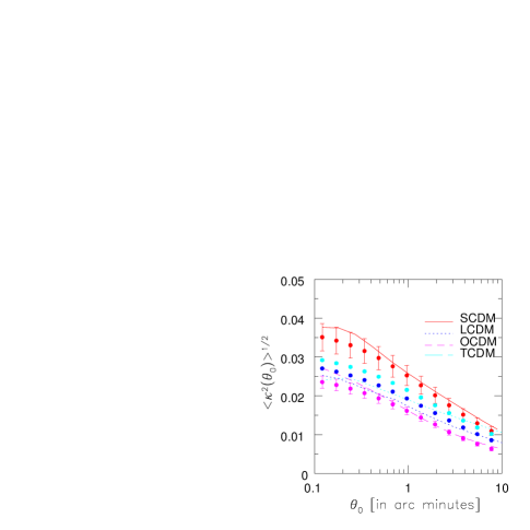
Figure 2: Analytical predictions for the r.m.s variance of the convergence field $\kappa(\theta_{0})$ are plotted against numerical ray tracing experiments as a function of the smoothing angle $\theta_{0}$. Solid, dotted, short-dashed and long-dashed lines correspond to theoretical predictions for the SCDM, LCDM, OCDM and TCDM models. Dots correspond to numerical computations averaged over several different realizations, with the error bars giving the scatter between different realizations.

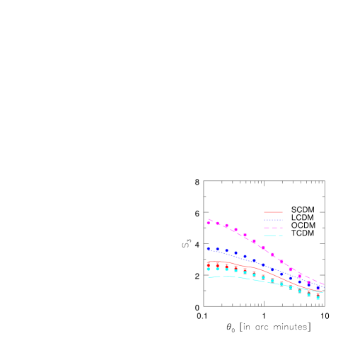
Figure 3: Analytical predictions for the normalized skewness $S_{3}$ of the smoothed convergence field $\kappa(\theta_{0})$. Solid, dotted, short-dashed and long-dashed lines correspond to theoretical predictions for the SCDM, LCDM, OCDM and TCDM models. Dots correspond to numerical computations averaged over several different realizations, with the error bars giving the scatter between different realizations. A hierarchical form is assumed for the 3-point correlation function of underlying dark matter distribution. The amplitude $Q_{3}$ is evaluated using hyper-extended perturbation theory (Scocciomarro & Frieman 1998).

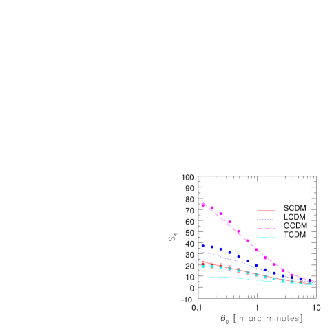
Figure 4: Analytical predictions for the normalized kurtosis $S_{4}$ of the smoothed convergence field $\kappa(\theta_{0})$. The lines and dots denote analytical and numerical results as in the preceding figures. The 4-point function is computed in analogy with the three-point function shown in figure 3.

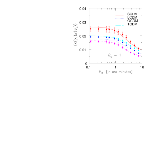
Figure 5: Analytical predictions for the correlation function $\langle\kappa(\gamma_{1})\kappa(\kappa_{2})\rangle$ of the smoothed convergence field $\kappa(\theta_{0})$ as a function of the separation angle $\theta_{12}$. The lines and dots denote analytical and numerical results as in the preceding figures. The smoothing angle is fixed at $\theta_{0}=1^{\prime}$.

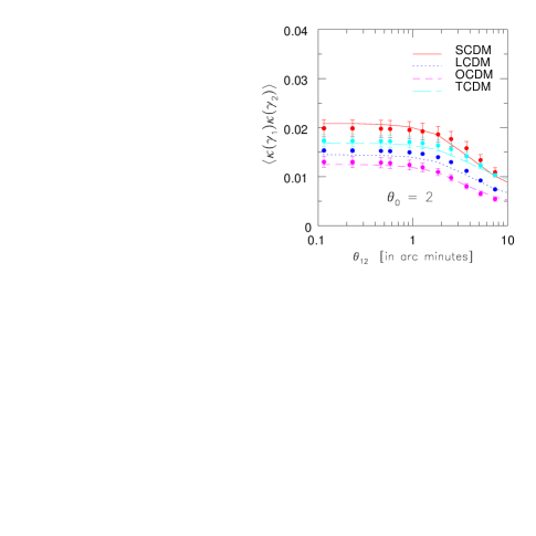
Figure 6: The correlation function $\langle\kappa(\gamma_{1})\kappa(\kappa_{2})\rangle$ is shown as in figure 5, but with smoothing angle $\theta_{0}=2^{\prime}$.

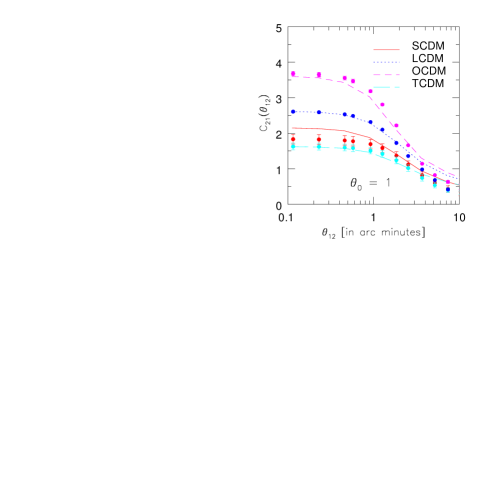
Figure 7: The third order cumulant correlator $C_{21}(\theta_{12})$ of the smoothed convergence field $\kappa(\theta_{0})$ is plotted as a function of the separation angle $\theta_{12}$. The lines and dots denote analytical and numerical results as in the preceding figures. The smoothing angle is $\theta_{0}=1^{\prime}$.

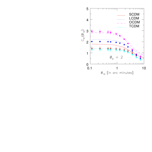
Figure 8: The third order cumulant correlator $C_{21}(\theta_{12})$ is shown as in figure 7, with smoothing angle $\theta_{0}=2^{\prime}$.

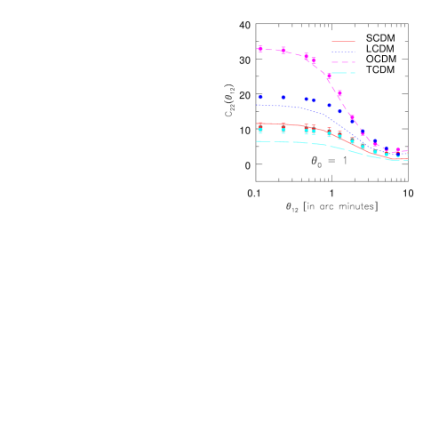
Figure 9: The fourth order normalized cumulant correlator $C_{22}(\theta_{12})$ as a function of separation angle $\theta_{12}$. The lines and dots denote analytical and numerical results as in the preceding figures. The amplitude $Q_{4}$ for the four-point correlation function is evaluated using hyper-extended perturbation theory. We used Bernardeau & Schaeffer’s (1992) model for the correlation hierarchy to separate the topological amplitudes $R_{a}$ and $R_{b}$.

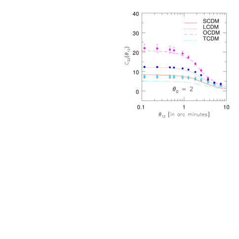
Figure 10: The fourth order normalized cumulant correlator $C_{22}(\theta_{12})$ as in figure 9, with smoothing angle $\theta_{0}=2^{\prime}$.

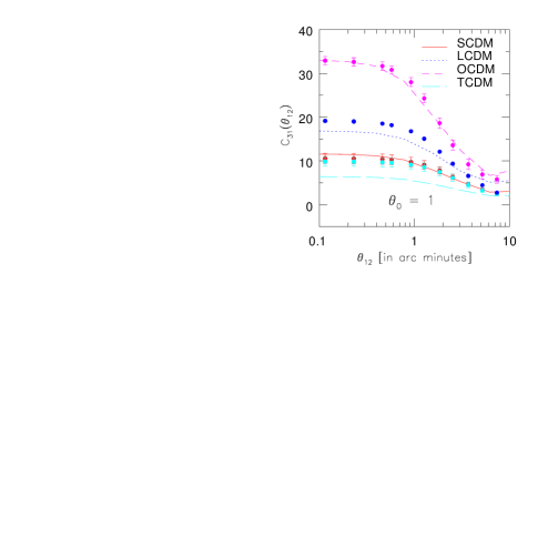
Figure 11: The fourth order normalized cumulant correlator $C_{31}(\theta_{12})$ of the smoothed convergence field $\kappa(\theta_{0})$ as a function of the separation angle $\theta_{12}$. The lines and dots denote analytical and numerical results as in the preceding figures. The smoothing angle is $\theta_{0}=1^{\prime}$.

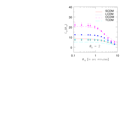
Figure 12: The fourth order normalized cumulant correlator $C_{31}(\theta_{12})$ as in figure 11, with smoothing angle $\theta_{0}=2^{\prime}$.

3.3 Modeling the non-linear power spectrum

In numerical computations of the variance and volume averages of higher order correlation functions, we have to include the effects of non-linearity in the evolution of the power spectrum. The evolution of density inhomogenieties introduces radial dependences in the expression for the power-spectrum. In linear theory it can be written as $P(k,{\chi})=a^{2}(\chi)F^{2}(\chi)P(k)=D_{+}^{2}(\chi)P(k)$. Where $D_{+}(\chi)$ is the linear growth factor for the evolution of density perturbations and $F(\chi)$ depends on the background geometry of the universe. Lahav et al. (1991) approximated it by the following fitting function:

$$F(\chi)={5\over 2}\Omega_{m}a(\chi)^{-1}\left[xf+{3\over 2}\Omega_{m}a(\chi)^{-1}+\Omega_{K}\right]^{-1}$$ (27)

$$x=1+\Omega(a(\chi)^{-1}-1)+\Omega_{\Lambda}(a^{2}(\chi)-1)\ ;\ f=\Big{(}{\Omega_{m}\over{a(\chi)x}}\Big{)}^{0.6}.$$ (28)

For $a=1$, ignoring the weak $\Omega_{\Lambda}$ dependence of the logarithmic growth factor, the above expression gives,

$$F(\chi=0)={5\over 2}\Omega_{m}(1+\Omega_{m}^{0.6}+{1\over 2}\Omega_{m}-\Omega_{\Lambda})^{-1}$$ (29)

On scales where the dimensionless power, $\triangle^{2}(k,\chi))=4\pi k^{3}P_{\delta}(k,\chi)$, is comparable to unity nonlinear corrections become important. This is more important for models with low values of $\Omega_{m}$. In the quasi-linear regime such corrections can be computed using perturbation theory. An alternative semi-analytical approach which maps the linear power spectrum to the non-linear spetrum was propsed by Hamilton et al (1991) and was subsequently developed by Nityananda & Padmanabhan (1991); Peackok & Dodds (1996), Jain, Mo & White (1995) and Padmanabhan et al. (1996)). This ansatz involves mapping the nonlinear spectrum for a given wave number $k$ to the linear spectrum at a wave number $k_{L}$ which are related to each other by $k_{L}=k(1+\triangle^{2}(k,\chi))^{-1/3}$. The accuracy of the results depend on the function $G$ which relates the nonlinear power on $k$ with the linear power spectrum $k_{L}$ i.e. $\triangle^{2}(k,\chi)=G[\triangle^{2}_{L}(k_{L},\chi)]$. We use the fitting formula of Peackock & Dodds (1996) to describe the non-linear power spectra as a function of length scale and redshift.

3.4 Modeling hierarchical amplitudes in the non-linear regime

As discussed above, different models for the hierarchical amplitudes predict different relations between the topological amplitudes that contribute to a given order, e.g. for the fourth order correlation functions we have two different topologies, the “snakes” and “stars”. Bernardeau & Schaeffer (1991) proposed that hybrid and snake topologies at a given order can be constructed from lower order topologies as the vertices of trees representing the correlation hierarchy obey a multiplicative relation. This will mean that $R_{a}=Q^{2}$. However note that the full prescription for $Q$, $R_{a}$ and other higher order “star” topologies will need a more detailed modeling of the non-linear density distribution. However it was noted by Munshi et al (1999) that since at each order we have only one new star topologies and $S_{N}$ parameters at each order are completely determined by the topological amplitudes of the same order, it is possible to determine these star topologies if we have a prescription to determine $S_{N}$ parameters at various order. In the quasi-linear regime perturbation theory provides such a formalism and Bernardeau (1992, 1994) developed a scheme to predict the $S_{n}$ parameters of arbitrary order in the quasi-linear regime using a tophat smoothing. Different extensions of perturbation theory have been suggested to predict the one-point statistics in the highly non-linear regime. Colombi et al (1996) proposed to replace the local spectral index $n$ in the expressions for the $S_{N}$ parameters with an effective spectral index $n_{eff}$. However it was realized that while the same $n_{eff}$ can be used for all $S_{N}$ for a given power spectrum, $n_{eff}$ does not coincide with the local slope of the non-linear power spectrum. Sccocimarro and Frieman (1998) on the other hand noted that the values of the $S_{N}$ parameters in the co-linear configuration in the quasi-linear regime describe the amplitudes for these quantities in the nonlinear regime in which they become shape independent. We use their hyper-extended perturbation theory (HEPT) to make concrete predictions for the $S_{N}$ parameters for weak lensing statistics. Their model for the dark matter distribution predicts:

$$S_{3}(n)=3\ {4-2^{n}\over 1+2^{n+1}}$$ (30)

$$S_{4}(n)=8\ {54-27~{}2^{n}+2~{}3^{n}+6^{n}\over 1+6~{}2^{n}+3~{}3^{n}+6~{}6^{n}}.$$ (31)

We find that our results for all $S_{N}$ parameters at arcminute scales are very accurately described by the local spectral index $n=-2.3$ for all four cosmological scenarios. HEPT is very accurate in predicting one point cumulants; it is possible to combine it the Benardeau & Schaeffer (1992) ansatz to compute the topological weights associated with different type of diagrams as well (see Munshi et al. 1999 for more details). This is necessary to predict the cumulant correlators or other multi-point statistics. HEPT gives us $Q_{3}=2.70$ and $Q_{4}=9.52$ for $n=-2.3$, and we get $R_{a}=7.29$ and $R_{b}=16.23$ for snake and star topologies, respectively. As noted by Munshi et al (1999), one can also use EPT as proposed by Colombi et al. (1996) which gives us very similar results. Finite volume N-body catalogs introduce a bias in the determination of the $S_{N}$ parameters (see.g. Colombi et al (1995)). In particular it has been noted that the $S_{N}$ parameters are biased towards lower values if determined from finite volume catalogs. Elaborate schemes were developed to correct such finite volume effects and were tested extensively against numerical simulations (Colombi et al. 1995; Munshi et al. 1997). Such effects will also be important in the determination of various statistical quantities from ray tracing simulations, which use the outputs of N-body simulations. We have not included finite volume corrections in our analysis of lower order cumulants and cumulant correlators. A detailed study of such corrections will be presented elsewhere.

4 Comparing analytical predictions with numerical simulations

4.1 Cumulants

Our study of one-pont statistics includes the variance, $S_{3}$ and $S_{4}$. We have computed these quantities as a function of smoothing angle ranging from $0.1^{\prime}$ to $10^{\prime}$. We have used approximately ten realizations for each cosmological model studied by us, except for the LCDM model where only one realization was used. Sources galaxies were taken to be at $z_{s}=1$. The use of such a large number of realizations gives us the opportunity to probe the degree of fluctuation from one realization to another. We find that our results are very accurately described by analytical approximations. Larger scales are more likely to be affected by the finite volume corrections described above. Compared to two-point statistics, one point cumulants are less affected by the finite size of the catalogs. In our analysis of one-point statistics, we find very good agreement between theory and numerical simulations, which suggests that such effects are indeed negligible. It is also to be noted that we have used the small angle approximation in our analytical computations, which is expected to hold good for the small angular scales studied by us.

In Figure 2 we plot the variance of the convergence field $\kappa^{2}{(\theta_{0})}$, smoothed with a tophat filter of smoothing angle $\theta_{0}$. The variance for the SCDM model is larger than in the other models. In most of the models the analytical predictions show a very good agreement with numerical results. Issues related to the effect of finite force resolution have been extensively dealt with in the study by Jain et al. (1999). We find that for all models a smoothing angle larger than $0.25^{\prime}$ is sufficient to remove such effects. Compared to other models, the TCDM models shows a slight departure from the analytical results; this could be due to the presence of large-scale power in this spectra. In Figures 3 and 4 we have plotted the next order normalized moments, $S_{3}$ and $S_{4}$. Again, the analytical models agree with the numerical results very well and it is also evident that the $S_{N}$ parameters can directly probe cosmological parameters, especially $\Omega_{0}$. At large smoothing angles one can see that analytical results start to overestimate the $S_{N}$ parameters. This is related to the fact that we have considered the hierarchical amplitudes constant with scale; in practice they go through a transition from the non-linear regime to the quasi-linear regime. Nonlinear estimates of the $S_{N}$ parameters based on EPT or HEPT therefore over-predict such amplitudes. Finite volume corrections also starts to become more important for larger smoothing scales. However despite such effects we find the agreement between analytical simulations and numerical results to be very good. A good match also indicates that the Born approximation is a very good approximation even for the smaller angular scales probed by us.

Throughout our studies of cumulants we have used top-hat filters for smoothing the convergence field $\kappa$. The analytical results we have presented here can easily be extended to other filters such as compensated filters, which may be more useful from an observational point of view. We hope to present results of such analyses elsewhere.

Cumulants are normalized moments of the one-point probability distribution function (PDF) for the convergence field. Our analytical prediction maps cumulants of the underlying dark matter distribution to that of the convergence field. In a similar analysis it is possible to map the complete PDF of the density to the convergence PDF (Munshi & Jain 1999)

4.2 Cumulant Correlators

We have measured cumulant correlators from simulations for two different smoothing angles, $\theta_{0}=1^{\prime}$ and $\theta_{0}=2^{\prime}$. For each $\theta_{0}$, several separation angles $\theta_{12}$ were considered, ranging from from $\theta_{12}=0.1^{\prime}$ to $\theta_{12}=10^{\prime}$. We have measured $C_{21}$ at third order and $C_{31}$ and $C_{22}$ at fourth order. For small separation angles when two patches overlap with each other, the cumulant correlators $C_{pq}$ become equal to the moments $S_{p+q}$. The numerical results for $C_{31}$ do correspond to $S_{3}$ and $C_{22}$ and $C_{31}$ correspond to $S_{4}$ at small angular scales.

In agreement with our findings for the one-point cumulants, we find that analytical approximations for cumulant correlators are very close to results obtained from numerical simulations. Figures 5 and 6 show the two point cumulant correlators, for smoothing angles $\theta_{0}=1^{\prime},2^{\prime}$ respectively, while figures 7 and 8 show the third order correlators. The fourth order correlator $C_{22}$ is shown in figures 9 and 10, with the same smoothing angles, and $C_{31}$ is shown in figures 11 and 12. Cumulant correlators are more strongly affected by finite volume correction compared to their one-point counterparts. We find that for large separation angles $\theta_{12}$, there are slight discrepancies between analytical and numerical results. The comparison can be more appropriately made by performing ray tracing experiments through bigger N-body boxes. It is also possible that for large angular scales, the corresponding physical scales are already in the quasilinear regime where the values of the hierarchical amplitudes are smaller than their values in the highly nonlinear regime.

Since the cumulant correlators are normalized moments of the two-point joint probability distribution function, they are directly related to two-point statistics of the underlying fields. They can also be related to the biasing of dark matter halos. The results of such an analysis will be presented elsewhere.

5 Discussion

Ongoing weak lensing surveys with wide field CCD are likely to produce shear maps on areas of order 10 square degrees. In the future, $10^{\circ}\times 10^{\circ}$ areas are also feasible, e.g. from the MEGACAM camera on the Canada France Hawaii Telescope and the VLT-Survey-Telescope. Ongoing optical (SDSS; Stebbins et al. 1997) and radio (FIRST; Kaminkowski et al. 1997) surveys can also provide useful imaging data for weak lensing surveys. Such surveys will provide a very useful map of the projected density of the universe and thus will help us test different dark matter models and probe the background geometry of the universe. They will also provide a unique opportunity to test different ansatze for gravitational clustering in the highly non-linear regime in an unbiased way. Traditionally such studies have used galaxy surveys, with the disadvantage that galaxies are biased tracers of the underlying mass distribution.

Most previous studies in weak lensing statistics used a perturbative formalism, which is applicable in the quasilinear regime and thus requires large smoothing angles. To reach the quasi-linear regime, survey regions must exceed areas of order 10 square degrees. Since existing CCD cameras typically have diameters of $0.25^{\circ}-0.5^{\circ}$, the initial weak lensing surveys are likely to provide us statistical information on small smoothing angles, of order $10^{\prime}$ and less. This makes the use of perturbative techniques a serious limitation, as the relevant physical length scales are in the highly nonlinear regime. We have employed a new technique based on the hierarchal ansatz to compute weak lensing statistics on these small angular scales. By combining the hierarchical ansatz with either hyper-extended or extended perturbation theory, we can make concrete predictions for one-point cumulants and many-point cumulant correlators (Munshi & Coles 1999). We found very good agreement between our non-linear analytical predictions and ray tracing results for angular scales ranging from sub arcminute to tens of arcminutes.

Our studies also indicate that several approximations involved in weak lensing studies are valid even in the highly non-linear regime of observational interest. While a weakly clustered dark matter distribution is expected to produce small deflections of photon trajectories, it is not clear if the effect of highly over-dense regions capable of producing large deflections can also be modeled using a hierarchal ansatz and the weak lensing approximation. Our study shows that this is indeed the case; the effect of density inhomogeneities on very small angular scales can be predicted with high accuracy using analytical approximations. Our study confirms for example that the Born approximation is valid in the highly nonlinear regime.

The two-point correlation functions and the projected power spectrum of the weak lensing convergence field $\kappa$ can be used to estimate the shape and normalization of the dark matter power spectrum. In this study we have shown that cosmological parameters can significantly affect higher order moments of the convergence field. Earlier studies have shown that the skewness of the convergence is sensitive to the cosmological matter density $\Omega_{m}$ in the quasilinear regime (Bernardeau, van Waerbeke & Mellier 1997; Jain & Seljak 1997; Schneider et al 1998), as well as in the nonlinear regime (Jain, Seljak & White 1999; Hui 1999). We have extended the work on higher order moments to include multi-point moments and fourth order moments. The multi-point moments may be more easily measured from non-contiguous lensing surveys. We find that the qualitative dependence of the skewness of $\kappa$ on $\Omega_{m}$ is present in these higher order statistics as well. In contrast, higher order moments of the underlying dark matter density fields are much less sensitive to background cosmological parameters (Jain, Seljak & White 1999).

The finite size of weak lensing catalogs will play an important role in the determination of cosmological parameters. It is therefore of interest to incorporate such effects in future analysis. Noise due to the intrinsic ellipticities of lensed galaxies will also need to be modeled. The present study is based on a top-hat window function which is easier to incorporate in analytical computations. It is possible to extend our study to other statistical estimators such as $M_{\rm ap}$, which use a compensated filter to smooth the shear field and may be more suitable for observational studies (Reblinsky et al 1999; Schneider et al 1997). Our method of computing cumulants and cumulant correlators can also be generalized to study the bias associated with the convergence field. Such studies will provide an interesting method of measuring the statistics of collapsed dark objects (e.g. Jain & Van Waerbeke 1999). We hope to present such results elsewhere.

It is interesting to consider an alternative to the hierarchical ansatz for the distribution of dark matter in the highly nonlinear regime. The dark matter can be modeled as belonging to halos with a mass function given by the Press-Schechter formalism, and spatial distribution modeled as in Mo & White (1996). When supplemented by a radial profile for the dark halos such a prescription can be used to compute the one-point cumulants of the convergence field. Reversing the argument, given the one point cumulants of the convergence field it is possible to estimate the statistics of dark halos.

The one-point probability distribution function and its two-point correlations are the complements to the moment hierarchy studied in this work. Numerical studies of the one point probability distribution function (pdf) of the convergence field have been carried out by Jain et al.(1999) and a fitting function has been provided by Yang (1999). Recently Valageas (1999a) and Munshi & Jain (1999) have computed the pdf of $\kappa$ using the hierarchical ansatz and compared the results to the measurements from simulations. The success of their analytical results means that the pdf for a desired cosmological model can be computed as a function of smoothing angle and redshift distribution. Thus physical effects, such as the magnification distribution for Type Ia Supernovae, can be conveniently computed. Thus we have a complete analytical description, based on models for gravitational clustering, for the full set of statistics of interest for weak lensing – the one point pdf, two point correlations, and the hierarchy of higher order cumulants and cumulant correlators. This analytical description has powerful applications in making predictions for a variety of models and varying the smoothing angle and redshift distribution of source galaxies; numerical studies are far more limited in the parameter space that can be explored.

6 Appendix

In our ray tracing simulations we have placed the source galaxies at a redshift of unity. However it is interesting to check how these results change when source redshift is altered. We find that the variance and other one point cumulants are sensitively dependent on the source redshift. While the variance increases with source redshift for a given smoothing angle, the $S_{N}$ parameters and the $C_{pq}$ parameters decrease with the increase in source redshift. For source redshifts $z_{s}<1$ the $S_{N}$ parameters are very sensitive to change in source redshifts. At low source redshifts, lensing probes the dark matter in the highly non-linear regime whereas for larger redshifts successive layers of matter tend to make the probability distribution function of $\kappa$ more Gaussian, thereby reducing the values of $S_{N}$ parameters. Nevertheless the ordering of the $S_{N}$ parameters in different cosmologies does not change with source redshifts. For any given source redshift the $S_{N}$ parameters are largest for open models and smallest for the TCDM model. Theoretical analysis by Valageas (1999b) has shown that for smaller source redshifts $S_{3}\propto z_{s}^{-1/2}$ and for larger source redshifts $S_{3}\propto(1+z_{s})^{-1}$. Our numerical results shows that this is indeed the case. Perturbative analyses of the dependence of the $S_{N}$ parameters on source redshift give qualitatively similar dependences.

In figure 13 we plot the variance for two different source redshifts $z_{s}=0.5$ and $z_{s}=1$. Figures 14 and 15 show $S_{3}$ and $S_{4}$ for redshifts $z_{s}=0.5$ and $z_{s}=2$; comparison with the same quantities for $z_{s}=1$ plotted in figures 3 and 4 shows that the $S_{N}$ parameters do decrease with source redshift for all smoothing angles. In figures 20 and 21 we have changed the source redshift continuously keeping the smoothing angles fixed at $\theta_{0}=1^{\prime}$ (left panels) and $\theta_{0}=2^{\prime}$ (right panels). The $S_{N}$ parameters show a rapid variation for small redshifts whereas for larger redshifts they vary at a much slower rate. The two point analogs of the variance and $S_{N}$ parameters i.e. the correlation function and $C_{pq}$ parameters shows a very similar pattern in their dependence on source redshifts. The two point correlation function $\kappa(\gamma_{1})\kappa(\gamma_{2})$ is plotted in figure 16 and the lower order cumulant correlators $C_{21}$, $C_{31}$ and $C_{22}$ in figures 17, 18 and 19, respectively. For small separation angles, i.e. small values of $\theta_{12}$, the cumulant correlators $C_{pq}$ match with their one-point counterparts, $S_{p+q}$.

In all of our plots we have assumed a specific form of the tree-level hierarchy as proposed by Bernardeau & Schaeffer (1992). The ansatz proposed by Szapudi & Szalay (1993) gives very similar results, as shown in figure 22. We have plotted $C_{22}$ and $C_{31}$ for $z_{s}=1$ (predictions for the third order cumulant correlator $C_{21}$ are the same for these ansatze).

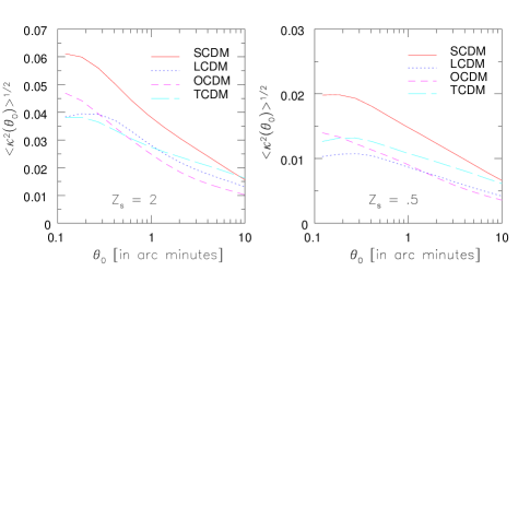
Figure 13: The variance $\langle\kappa^{2}(\theta_{0})\rangle$ as a function of smoothing angle $\theta_{0}$ for two different redshifts. Note that the variance increases with source redshift whereas all $S_{N}$ parameters decrease with redshift.

Figure 14: The normalized skewness $S_{3}$ as a function of the smoothing angle $\theta_{0}$ for two different redshifts. $S_{3}$ is higher for lower source redshift due to smaller projection effects and greater nonlinear clustering of the lensing matter.

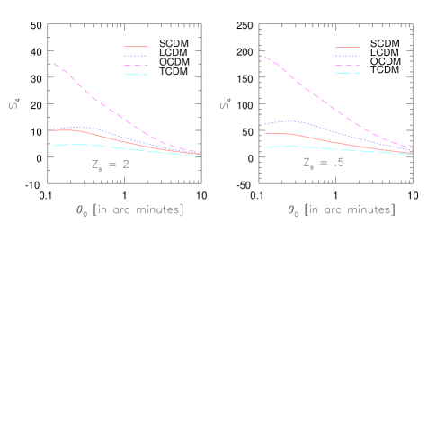
Figure 15: The normalized kurtosis parameter $S_{4}$ as a function of smoothing angle $\theta_{0}$ for two different source redshifts. Note that the ordering of the different curves does not change with source redshift. The $S_{N}$ paraneters are largest for the OCDM model and smallest for the TCDM model for any given redshift.

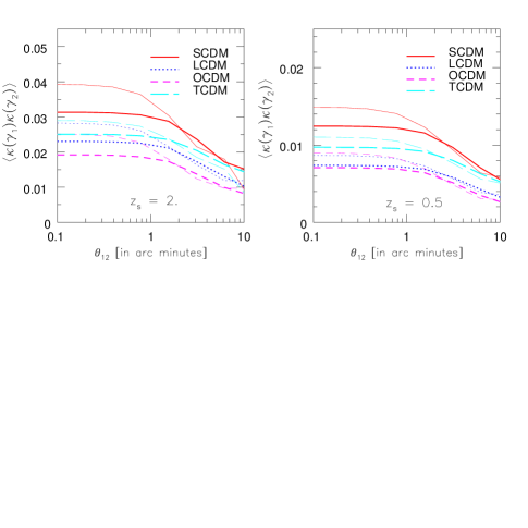
Figure 16: The correlation function $\langle\kappa(\gamma_{1})\kappa(\gamma_{2})\rangle$ as a function of separation angle $\theta_{12}$ for two different source redshifts $z_{s}$. The smoothing angles are $\theta_{0}=1^{\prime},2^{\prime}$ for the upper and lower curves at small $\theta_{12}$, respectively.

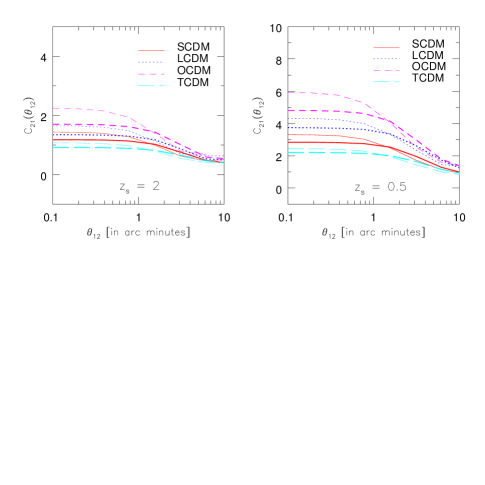
Figure 17: The third order cumulant correlator $C_{21}$ as a function of separation angle $\theta_{12}$, for two different source redshifts $z_{s}$. The dependence of the cumulant correlators $C_{pq}$ on redshift is very similar to their one-point counterpart.

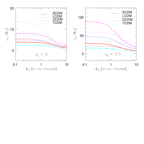
Figure 18: The fourth order cumulant correlator $C_{31}$ for two different source redshifts $z_{s}$ as a function of separation angle $\theta_{12}$. The smoothing angles are $\theta_{0}=1^{\prime},2^{\prime}$ for the upper and lower curves at small $\theta_{12}$, respectively. The $C_{pq}$ parameters tend to increase for low source redshift like the $S_{N}$ paramters.

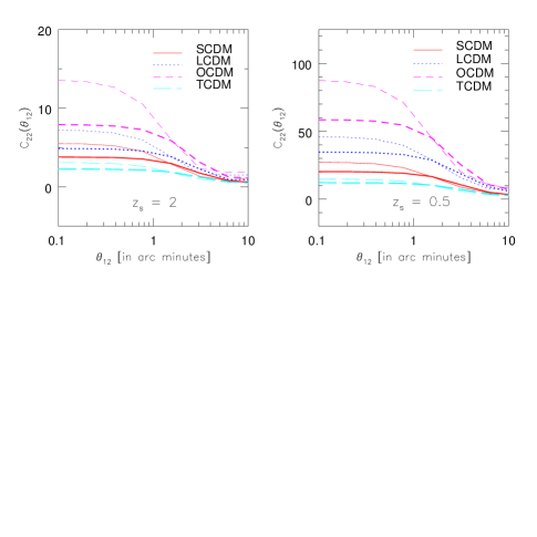
Figure 19: The fourth order cumulant correlator $C_{22}$ for two different source redshifts $z_{s}$ as a function of separation angle $\theta_{12}$.

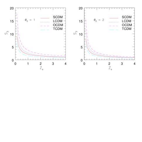
Figure 20: Variation of $S_{3}$ with source redshift $z_{s}$ for fixed smoothing angle $\theta_{0}=1^{\prime}$ in the left panel and $\theta_{0}=2^{\prime}$ in the right panel. While the rate of increase is moderate for high redshifts the rate is much more rapid at smaller redshift. The growth of density inhomogeneities at lower redshifts causes the values of the $S_{N}$ parameters to increase, while for larger redshifts subsequent layers of lensing matter tend to make the probability distribution function more Gaussian.

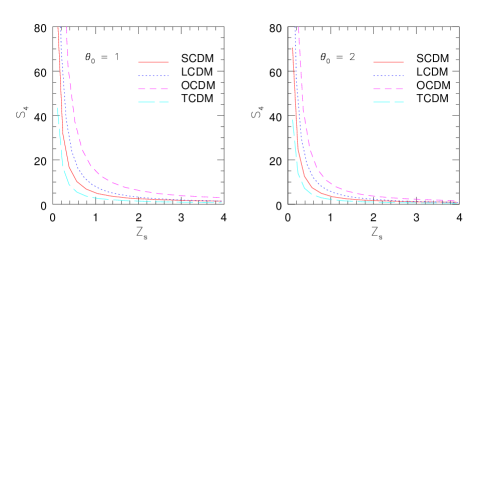
Figure 21: Variation of $S_{4}$ with source redshift $z_{s}$ for fixed smoothing angle $\theta_{0}=1^{\prime}$ in the left panel and $\theta_{0}=2^{\prime}$ in the right panel.

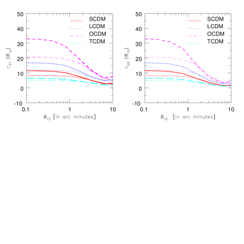
Figure 22: The analytical predictions for the cumulant correlators $C_{22}$ and $C_{31}$ are plotted using the Szapudi & Szalay (1993) ansatz $R_{a}=R_{b}$ in combination with hyper-extended perturbation theory. The smoothing angles are $\theta_{0}=1^{\prime},2^{\prime}$ for the upper and lower curves at small $\theta_{12}$, respectively. We find that the predictions are almost identical to that of Bernardeau & Schaeffer’s ansatz, although the two differ in the way they assign amplitudes to trees of different topologies of the same order.

References

- [1] Babul, A., & Lee, M.H., 1991, MNRAS, 250, 407
- [2] Balian R., Schaeffer R., 1989, A& A, 220, 1
- [3] Bartelmann M., Huss H., Colberg J.M., Jenkins A.
- [4] Bartelmann, M. & Schneider, P., 1991, A& A, 248, 353 Pearce F.R., 1998, A&A, 330, 1
- [5] Bernardeau F., 1992, ApJ, 392, 1
- [6] Bernardeau F., 1999, astro-ph/9901117
- [7] Bernardeau F., Schaeffer R., 1992, A& A, 255, 1
- [8] Bernardeau F., Schaeffer R., 1999, astro-ph/9903087
- [9] Bernardeau F., van Waerbeke L., Mellier Y., 1997, A& A, 322, 1
- [10] Blandford R.D., Saust A.B., Brainerd T.G., Villumsen J.V., 1991, MNRAS, 251, 600
- [11] Boschan P., Szapudi I., Szalay A.S., 1994, ApJS, 93, 65
- [12] Couchman H.M.P., Barber A.J., Thomas P.A., 1998, astro-ph/9810063
- [13] Davis M., Peebles P.J.E., 1977, ApJS, 34, 425
- [14] Fry, J.N., 1984, ApJ, 279, 499
- [15] Fry, J.N., & Peebles, P.J.E., 1978, ApJ, 221, 19
- [16] Groth, E., & Peebles, P.J.E., 1977, ApJ, 217, 385
- [17] Gunn, J.E., 1967, ApJ, 147, 61
- [18] Hamilton A.J.S., Kumar, P., Lu, E. & Matthews, A., 1991, ApJ, 374, L1
- [19] Hui, L., astro-ph/9902275
- [20] Hui, L., & Gaztanaga, astro-ph/9810194
- [21] Jain, B., Mo H.J., & White S.D.M., 1995, MNRAS, 276, L25
- [22] Jain, B., & Seljak, U., 1997, ApJ, 484, 560
- [23] Jain, B., & Van Waerbeke, 1999, astro-ph/9910459
- [24] Jain, B., Seljak, U., White, S.D.M., 1999, astro-ph/9901191
- [25] Jaroszyn’ski, M., Park, C., Paczynski, B., & Gott, J.R., 1990, ApJ, 365, 22
- [26] Jaroszyn’ski, M. 1991, MNRAS, 249, 430
- [27] Kaiser, N., 1992, ApJ, 388, 272
- [28] Kaiser, N., 1998, ApJ, 498, 26
- [29] Limber D.N., 1954, ApJ, 119, 665
- [30] Lee, M.H., & Paczyn’ski B., 1990, ApJ, 357, 32
- [31] Miralda-Escudé J., 1991, ApJ, 380, 1
- [32] Mo, H., White, S.D.M., 1996, MNRAS, 282, 347
- [33] Munshi D., Bernardeau F., Melott A.L., Schaeffer R., 1999, MNRAS, 303, 433
- [34] Munshi D., Melott A.L, 1998, astro-ph/9801011
- [35] Munshi D., Coles P., Melott A.L., 1999a, MNRAS, in press, astro-ph/9812337
- [36] Munshi D., Coles P., Melott A.L., 1999b, MNRAS, in press, astro-ph/9902215
- [37] Munshi D., Melott A.L., Coles P., 1999c, MNRAS, in press, astro-ph/9812271
- [38] Munshi D. & , Coles P., 1999, MNRAS, in press
- [39] Munshi D. & , Jain B., 1999, MNRAS, submitted, astro-ph/9911502
- [40] Mellier Y., 1999, astro-ph/9901116
- [41] Nityananda R., & Padamanabhan T., 1994, MNRAS, 271, 976
- [42] Padmanabhan T., Cen R., Ostriker J.P., Summers, F.J., 1996, ApJ, 466, 604
- [43] Premadi P., Martel H., Matzner R., 1998, ApJ, 493, 10
- [44] Press, W.H., & Schechter, P. 1974, ApJ, 187, 425
- [45] Peebles P.J.E., 1980, The Large Scale Structure of the Universe. Princeton University Press, Princeton
- [46] Reblinsky, K., Kruse, G.,Jain, B., Schneider, P., astro-ph/9907250
- [47] Schneider, P., & Weiss, A., 1988, ApJ, 330,1
- [48] Schneider, P., van Waerbeke, L., Jain, B. & Kruse, G. 1998, MNRAS, 296, 873, 873
- [49] Scoccimarro R., Colombi S., Fry J.N., Frieman J.A., Hivon E., Melott A.L., 1998, ApJ, 496, 586
- [50] Scoccimarro R., Frieman J., 1998, preprint, astro-ph/9811184
- [51] Szapudi I., Colombi S., 1996, ApJ, 470, 131
- [52] Szapudi I., Szalay A.S., 1993, ApJ, 408, 43
- [53] Szapudi I., Szalay A.S., 1997, ApJ, 481, L1
- [54] Szapudi I., Szalay A.S., Boschan P., 1992, ApJ, 390, 350
- [55] Valageas, P., 1999a, astro-ph/9904300
- [56] Valageas, P., 1999b, astro-ph/9911336
- [57] van Waerbeke, L., Bernardeau, F., Mellier, Y., 1998, astro-ph/9807007
- [58] Wambsganss, J., Cen, R., & Ostriker, J.P., 1998, ApJ, 494, 298
- [59] Wambsganss, J., Cen, R., Xu, G. & Ostriker, J.P., 1997, ApJ, 494, 29
- [60] Wambsganss, J., Cen, R., Ostriker, J.P. & Turner, E.L., 1995, Science, 268, 274
- [61] Wang Y., 1999, ApJ, in press.