Statistical analysis of large–scale structure in the Universe

Abstract

Methods for the statistical characterization of the large–scale structure in the Universe will be the main topic of the present text. The focus is on geometrical methods, mainly Minkowski functionals and the $J$–function. Their relations to standard methods used in cosmology and spatial statistics and their application to cosmological datasets will be discussed. A short introduction to the standard picture of cosmology is given.

1 Introduction

A fundamental problem in cosmology is to understand the formation of the large–scale structure in the Universe. Normally theoretical models of large–scale structure, whether involving analytical predictions or numerical simulations, are based on some form of random or stochastic initial conditions. This means that a statistical interpretation of clustering data is required, and that statistical tools must be deployed in order to discriminate between different cosmological models. Moreover the identification and characterization of specific geometric features in the galaxy distribution like walls, filaments, and clusters will deepen our understanding of structure formation, assist in the construction of approximations and also help to constrain cosmological models.

During the past two decades enormous progress has been made in the mapping of the distribution of galaxies in the Universe. Using the measured redshifts of galaxies as distance indicators, and knowing their angular positions on the sky, we can obtain a three–dimensional view of the distribution of luminous matter in the Universe. Presently available redshift surveys already permit the detailed study of the statistical properties of the spatial distribution of galaxies. Surveys of galaxy redshifts that cover reasonable solid angles and are significantly deeper than those presently available present important challenges, and not just for the observers. A precise definition of the statistical methods is needed to extract most out of the costly data, and this is an important goal for theorists.

A complete review of the variety of statistical methods used in cosmology is not attempted. The focus of this overview will be on methods of point process statistics using geometrical ideas like Minkowski functionals and the $J$–function; moment based methods will also be mentioned. For reviews with a different emphasis see e.g. Peebles (1980), Bertschinger (1992), Peacock (1992), Borgani (1995), Efstathiou (1996), and Martínez (1996).

This text is organized as follows:
In Sect. 2 we will give a short introduction to the common theoretical “prejudice” in cosmology and describe some observational issues. We briefly comment on two–point correlations (Sect. 3.1) and moment based methods (Sect. 3.2), and focus on Minkowski functionals (Sect. 3.3) and the $J$–function, as well as its extensions the $J_{n}$–functions (Sect. 3.4). In Sect. 4 we summarize and provide an outlook.

2 Cosmological models and observations

Most cosmological models studied today are based on the assumption of homogeneity and isotropy (see however Buchert and Ehlers 1997 and Buchert 1999). Observationally one can find evidence that supports these assumptions on very large scales, the strongest being the almost perfect isotropy of the cosmic microwave background radiation (after assigning the whole dipole to our proper motion relative to this background). The relative temperature fluctuations over the sky are of the order of $10^{-5}$ as shown in Fig. 1. This tells us that the Universe was nearly isotropic and, with some additional assumptions, homogeneous at the time of decoupling of approximately 13Gy (Giga years) ago.

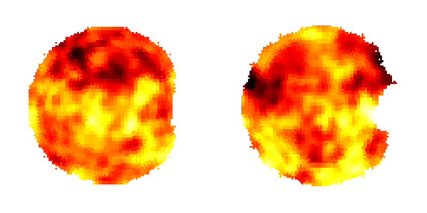
Figure 1: Projection of the temperature fluctuations in the microwave background radiation as observed by the COBE satellite (from Schmalzing and Górski 1998). The relative fluctuations are of the order of $10^{-5}$.

For such a highly symmetric situation the universal expansion may be described by a position vector ${\mathbf{x}}_{H}(t)$ at time $t$ that can be calculated from the initial position ${\mathbf{x}}_{i}$

$${\mathbf{x}}_{H}(t)=a(t)\ {\mathbf{x}}_{i}$$ (1)

using the scale factor $a(t)$ with $a(t_{i})=1$. The dynamical evolution of $a(t)$ is determined by the Friedmann equations (see e.g. Padmanabhan 1993). As a direct consequence the velocities may be approximated by the Hubble law,

$${\mathbf{v}}_{H}(t)=H(t)\ {\mathbf{x}}_{H}(t)$$ (2)

relating the distance vector ${\mathbf{x}}_{H}(t)$ with the velocity ${\mathbf{v}}_{H}(t)$ by the Hubble parameter $H(t)={\dot{a}}(t)/a(t)$. Indeed such a mainly linear relationship is observed for galaxies (see Fig. 2). The deviations visible may be assigned to peculiar motions, as caused by mass density perturbations.

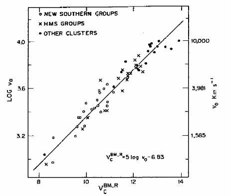
Figure 2: Hubble law for galaxy clusters and groups taken from (Sandage, 1995). The $x$–axis is proportional to distance indicator obtained from the a certain luminosity of the clusters and groups, whereas the $y$–axis is proportional to the redshift.

However, on small and on intermediate scales up to several hundreds of Mpcs, there are significant deviations from homogeneity and isotropy as visible in the spatial distribution of galaxies. (Mega parsec (Mpc) is the common unit of length in cosmological applications with 1pc=3.26 light years.) Large holes, filamentary as well as wall–like structures are observed (Fig. 3, see also sect. 3.3.4).

Figure 3: In the upper two panels, the position of the galaxies in two neighboring slices with an angular extent of $135\times 5$ deg², and a maximum distance of 120$h^{-1}$Mpc from our galaxy which is located at the tip of the cone. The galaxies are shown projected along the angular coordinate spanning only 5deg. In the lower plot both slices are shown projected on top of each other (data from Huchra et al. 1990 and Huchra et al. 1995).

One of the goals in cosmology is to understand how these large scale structures form, given a nearly homogeneous and isotropic matter distribution at some early time. In the Newtonian approximation the process of structure formation is modeled using a self gravitating pressure–less fluid, with the mass density $\varrho({\mathbf{x}},t)$ and the velocity field ${\mathbf{v}}({\mathbf{x}},t)$:

$$\partial_{t}\varrho+\nabla(\varrho{\mathbf{v}}) =0,$$

$$\partial_{t}{\mathbf{v}}+({\mathbf{v}}\cdot\nabla){\mathbf{v}} ={\mathbf{g}},$$

$$\nabla\times{\mathbf{g}} =0,$$ (3)

$$\nabla\cdot{\mathbf{g}} =-4\pi G\varrho.$$

The first equation is the continuity equation, stating mass–conservation, the second comes from momentum conservation with the gravitational acceleration ${\mathbf{g}}({\mathbf{x}},t)$ self–consistently determined from the mass density. With small fluctuations in $\varrho$ and ${\mathbf{v}}$ given at some early time, this system of partial differential equations constitutes a highly non–linear initial value problem. Up to now no general solution is known. Approximate solutions may be constructed using a perturbative expansion around the homogeneous background solutions either for the fields $\varrho$ and ${\mathbf{v}}$ directly or for the characteristics. The first one is called Eulerian perturbation theory (see e.g. Peebles 1980), whereas the second is named Lagrangian perturbation theory (see e.g. Buchert 1996). Also numerical integration with N–body simulations is used.

The initial conditions are often chosen as realization of a Gaussian random field for the density contrast $(\varrho-\varrho_{H})/\varrho_{H}$. In principle a Gaussian random field model for the density contrast allows for unphysical negative mass densities, however we find that the initial fluctuations in the mass density are by a factor of $10^{5}$–times smaller than the mean value of the field, and therefore negative densities are practically excluded. Using the methods mentioned above we can follow the nonlinear time evolution of the density field, leading to a highly non–Gaussian field. In this evolved mass density field galaxies are identified sometimes also utilizing the velocity field. Moreover, our understanding of the physical processes determining the galaxy formation is still limited.

Two popular stochastic models used to describe the distribution of galaxies are the Poisson model and the peak selection. In the Poisson model we assume that the mean number of galaxies inside a region $C$ is directly proportional to the total mass inside this region (see e.g.  Peebles 1980, often also called Poisson sampling). Hence the intensity measure $\Lambda(C)$ – the mean number of galaxies inside $C$ – is

$$\Lambda(C)\propto\int_{C}{\rm d}{\mathbf{x}}\ \varrho({\mathbf{x}}).$$ (4)

If the mass density $\varrho$ is modeled as a random field the Poisson model results in a double–stochastic point process, i.e. a Cox process (Stoyan et al., 1995).

Within the peak selection model, galaxies appear only at the peaks of the density field above some given threshold (Bardeen et al., 1986). This model is an example for an “interrupted point process” (Stoyan et al., 1995). In Figure 4 we illustrate both models in the one–dimensional case.

Figure 4: The left figure illustrates the Poisson model, whereas the right figure shows the peak selection for the same density field.

There are also dynamically and micro–physically motivated models for the identification of galaxies in simulations we do not cover here (Kates et al. 1991, Weiß and Buchert 1993, Kauffmann et al. 1997).

As we have seen several “parameters” enter these partly deterministic, partly stochastic models for the galaxy distribution. Before describing the statistical methods used to constrain these parameters, typical observational problems entering the construction of galaxy catalogues will be mentioned.

The starting point is the two–dimensional distribution of galaxies on the celestial sphere. Their angular positions are known to a high precision compared to their radial distance $r$. In most galaxy catalogues the radial distance is estimated utilizing the redshift:

$$z=\frac{\lambda_{\rm obs}-\lambda_{\rm lab}}{\lambda_{\rm lab}},$$ (5)

with the observed wavelength of a spectral line $\lambda_{\rm obs}$ and with the wavelength of the same spectral line measured in a laboratory $\lambda_{\rm lab}$. Out to several hundreds of Mpc’s the relation between the radial distance $r$ and the redshift $z$ is to a good approximation

$${\rm c}z\approx|v_{H}|+u=H_{0}r+u,$$ (6)

with the velocity of light c, and the Hubble parameter $H_{0}$ at present time (see (2)). $u$ is the radial component of the peculiar velocity, i.e. the local deviation from the global expansion due to inhomogeneities. Galaxy catalogues sampled homogeneously and with $r$ determined independently from the redshift are still rare. Therefore the distance is simply estimated by

$$r=\frac{{\rm c}z}{H_{0}},$$ (7)

neglecting the peculiar velocities $u$. This is often called “working in redshift space”. There is still some controversy about the actual value of the Hubble parameter which is parameterized by the number $h$: $H_{0}=h\ 100$km sec^-1 Mpc^-1. Likely values are in the range $h=0.5-0.8$.

Furthermore we have to face another problem. The majority of galaxy catalogues is flux (i.e.  magnitude) limited. This means that the catalogue is complete for galaxies with a flux higher than some minimum flux $f_{\rm min}$. As a first approximation the absolute luminosity $L$ of a galaxy with observed flux $f_{\rm obs}$ at distance $r$ may be calculated by $L=4\pi r^{2}\ f_{\rm obs}$. Hence at larger distances we observe only the brightest galaxies as can be seen in Figure 5, resulting in a systematically in–homogeneously sampled point–set in three dimensions.

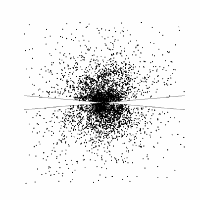
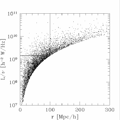
Figure 5: In the left figure the spatial distribution of the galaxies taken from the IRAS 1.2Jy galaxy catalogue (Fisher et al., 1995), projected along one axis. The horizontally cones indicate the region where the observation was obscured due to the absorption in our own galaxy. In the right plot the absolute luminosity of a galaxy against its radial distance is shown, each point represents one galaxy. The volume limited subsample with limiting distance of 100$h^{-1}$Mpc  includes only the galaxies in the marked upper left corner of the figure.

To construct a homogeneously sampled point set from such a galaxy catalogue we may restrict ourselves to galaxies closer than $r_{\rm lim}$ with a absolute luminosity higher than $L_{\rm lim}=4\pi r^{2}\ f_{\rm min}$. This procedure is called “volume limitation”. Such a set of galaxies for $r_{\rm lim}=100{h^{-1}{\rm Mpc}}$ is marked in Figure 5 and the spatial distribution is shown in Figure 6.

Figure 6: The spatial distribution of IRAS galaxies in a volume limited sample with a depth of 100$h^{-1}$Mpc, projected along one coordinate axis. This volume limited sample is formed by the galaxies shown in the upper left corner of the plot with luminosity against radial distance (Figure 5).

Especially in the direction of the disc of our galaxy, in the galactic plane, we suffer from extinction mainly due to dust. To take care of this we use a cut of 5 to 30 degrees (depending on the catalogue under consideration) around the galactic plane, resulting in a deformed sampling window as it can be seen in Figure 6.

The following discussion will refer to a set of points $X=\{{\mathbf{x}}_{i}\}_{i=1}^{N}$. The objects located at these points are either galaxies, or galaxy clusters, and also super–clusters (clusters of galaxy clusters). Galaxies are well defined objects in space, with an extent of typically 0.03$h^{-1}$Mpc. Similarly, galaxy clusters are well defined objects, clearly visible in the two–dimensional distribution of galaxies, with a typical extent of 1-3$h^{-1}$Mpc. Whether the combination of galaxy clusters to super–clusters is a reasonable concept is still some matter of debate (Kerscher, 1998b).

3 Statistics of large scale structure

New observations of our Universe will give us an increasingly precise mapping of the galaxy distribution around us (Gunn 1995, Maddox 1998). But we will have only one realization. This makes a statistical analysis problematic, especially model assumptions like stationarity (homogeneity) and isotropy may be tested locally only. For an interesting discussion of such problems see Matheron (1989). Still, global methods like the Minkowski functionals give us information on the shape and topology of this point set.

A pragmatic interpretation is that with a statistical analysis of a galaxy catalogue, one wants to constrain parameters of the cosmological models. These models incorporate some randomness, quantifying our ignorance of the initial conditions, or our limited understanding of the exact physical processes leading to the formation of galaxies.

3.1 Two–point statistics

Second–order statistics, also called two–point statistics, are still among the major tools to characterize the spatial distribution of galaxies. With the mean number density, or intensity, denoted by $\rho$, the product density

$$\rho_{2}({\mathbf{x}}_{1},{\mathbf{x}}_{2}){\rm d}V({\mathbf{x}}_{1}){\rm d}V({\mathbf{x}}_{2})=\rho^{2}g(r)\ {\rm d}V({\mathbf{x}}_{1}){\rm d}V({\mathbf{x}}_{2})$$ (8)

describes the probability to find a point in the volume element ${\rm d}V({\mathbf{x}}_{1})$ and another point in ${\rm d}V({\mathbf{x}}_{2})$, at the distance $r=|{\mathbf{x}}_{1}-{\mathbf{x}}_{2}|$; $|\cdot|$ is the Euclidean norm (we assume stationarity and isotropy). The product density $\rho_{2}({\mathbf{x}}_{1},{\mathbf{x}}_{2})$ is the Lebesgue density of the second factorial moment measure (e.g. Stoyan et al. 1995). Often the (full) two–point correlation function, also called pair correlation function, $g(r)$ and the normed cumulant $\xi_{2}(r)=g(r)-1$ are considered. Throughout the cosmological literature $\xi_{2}(r)$ is also called (two–point) correlation function (Peebles, 1980). For a Poisson process one has $g(r)=1$. Closely related is the correlation integral $C(r)$ (e.g. Grassberger and Procaccia 1984), the average number of points inside a ball of radius $r$ centred on a point of the distribution

$$C(r)=\int_{0}^{r}{\rm d}s\ \rho\ 4\pi s^{2}g(s),$$ (9)

which is related by $K(r)=C(r)/\rho$ to Ripley’s $K$ function, see Stoyans’s paper in this volume. Another common way to characterize the second–order properties is the excess fluctuation of the number density inside of $C$ with respect to a Poisson process:

$$\sigma^{2}(C)=\frac{1}{|C|^{2}}\int_{C}{\rm d}{\mathbf{x}}\int_{C}{\rm d}{\mathbf{y}}\ \xi_{2}(|{\mathbf{x}}-{\mathbf{y}}|).$$ (10)

Often the power spectrum $P(k)$ is used to quantify the second order statistical properties of the point distribution (Peebles, 1980). $P(k)$ may be defined as the Fourier transform of $\xi_{2}(r)=g(r)-1$:

$$P(k)=\frac{1}{(2\pi)^{3}}\ \int{\rm d}{\mathbf{x}}\ {\rm e}^{-i{\mathbf{k}}\cdot{\mathbf{x}}}\xi_{2}(|{\mathbf{x}}|),$$ (11)

with $k=|{\mathbf{k}}|$.

Observed two–point correlations

The first analysis of a galaxy catalogue using the two–point correlation function was presented by Totsuji and Kihara (1969). Following the work of Peebles (1973), today the two–point correlation function has become the standard tool, applied to nearly every cosmological dataset. The need for boundary corrected estimators was recognized early. Several estimators have been introduced, with differing claims on their applicability (Landy and Szalay 1993, Hamilton 1993, Stoyan and Stoyan 2000, Kerscher 1999, Pons–Bordería et al. 1999). A clarification for cosmological applications is attempted in Kerscher et al. (1999b).

Fig. 7 shows the (full) correlation function $g(r)$ and the normed cumulant $\xi_{2}(r)$ determined from a volume limited sample of the Southern Sky Redshift Survey 2 (SSRS2; da Costa et al. 1998) with 1179 galaxies. The strong clustering of galaxies, due to their gravitational interaction, is shown by large values of $g(r)$ and $\xi_{2}(r)$ for small $r$.

Figure 7: Estimated two–point correlation function $g(r)$ (solid) and the normed cumulant $\xi_{2}(r)=g(r)-1$ (dashed) in a double logarithmic plot for the volume limited sample from the SSRS2 with 100$h^{-1}$Mpc depth. The results of the minus (reduced–sample) estimator and the Fiksel (1988) estimator are shown, illustrating that only on large scales differences occur. The straight lines correspond to $g(r)\propto r^{-1}$ (solid) and $\xi_{2}(r)\propto r^{-1.81}$ (dashed).

Of special physical interest is, whether the two–point correlations are scale–invariant. A scale–invariant $g(r)\propto r^{D-3}$ is an indication for a fractal distribution of the galaxies (Mandelbrot 1982, Sylos Labini et al. 1998). A scale–invariant $\xi_{2}(r)\propto r^{-\gamma}$ is expected in critical phenomena (see Goldenfeld 1992, Gaite et al. 1999).

Now lets look at the log–log plot in Figure 7. Willmer et al. (1998) give a scale–invariant fit of $\xi_{2}(r)\propto r^{-\gamma}$ with a scaling exponent $\gamma=1.81$ in the range of 3-12$h^{-1}$Mpcfor the volume limited sample with 100$h^{-1}$Mpc. However on smaller scales the slope of $\xi_{2}$ is flattening, suggesting that a scale–invariant function $\propto r^{-\gamma}$ gives only a poor description of the observed $\xi_{2}(r)$ in this SSRS2–sample. If we look at the correlation function $g(r)$ in Figure 7, the observed data may be approximated by $g(r)\propto r^{3-D}$ with $D=2$ over the larger range from 0.5-20$h^{-1}$Mpc. However the scale–invariance of $g(r)$ is observed over less than 2 decades only, and therefore an estimate of a fractal dimension $D$ from the scaling exponent of $g(r)$ may be misleading (Stoyan 1998, McCauley 1997, McCauley 1998, Kerscher 1999). On large scales the observed $g(r)$ also deviates from a purely scale invariant model, and shows a tendency towards unity. This however depends on the estimator chosen. In this specific sample, a scale–invariant $g(r)$ seems to be suitable, but this is not so clear from other data sets. Also the result on small scales might be unreliable due to the small number of pairs with a short separation. For a comprehensive analysis of the SSRS2 catalogue focusing on two–point properties and scaling see Cappi et al. (1998).

Hence, currently we cannot exclude a scale–invariant $g(r)$, a scale–invariant $\xi_{2}(r)$, or no scale–invariance at all, with the limited observational range provided by the available three–dimensional catalogues. Hopefully this controversial issue will be clarified in the near future by the advent of deeper galaxy catalogues (Gunn 1995, Maddox 1998).

3.2 Higher moments

The two–point correlation function plays an important role in cosmology, since the inflationary paradigm suggests that the initial deviations from the homogeneous density field may be modeled as a Gaussian random field, stochastically completely specified by its mean density and its two–point correlation function (see e.g. Börner 1993). The analogous construction for point distributions is the Gauss–Poisson process (Milne and Westcott, 1972), with subtle but important differences from the Gaussian random field model. However, the nonlinear evolution of the mass density given by (3) generates high order correlations, not explainable within a Gaussian model. Hence, assuming an initial Gaussian density field, these higher order correlations give us information on the process of structure formation.

To investigate these nonlinear structures several methods are used. In the Sections 3.3 and 3.4 we will focus on morphological tools like the Minkowski functionals and on the $J$–function. A geometrical method we do not cover in this text is percolation analysis as introduced to cosmology by Shandarin (1983) (see also Sahni et al. 1997). Yet another one is the analysis based on the minimal spanning tree (Barrow et al. 1985, Doroshkevich et al. 1999). A description of the direct, moment based methods employed in cosmology is given now (Peebles, 1980):

As a generalization of the product density (8) one considers $n$–th order product densities

$$\rho_{n}({\mathbf{x}}_{1},\ldots,{\mathbf{x}}_{n})\ {\rm d}V_{1}\ldots{\rm d}V_{n}.$$ (12)

giving the probability of finding $n$ points in the volume elements ${\rm d}V_{1}$ to ${\rm d}V_{n}$, respectively. Again $\rho_{n}$ is the Lebesgue densities of the $n$–th factorial moment measures (Stoyan et al., 1995). In physical applications the (normalized) cumulants are often considered. As an example we look at the three–point correlations:

$$\rho_{3}({\mathbf{x}}_{1},{\mathbf{x}}_{2},{\mathbf{x}}_{3})=\rho^{3}\Big{(}1+\xi_{2}(|{\mathbf{x}}_{1}-{\mathbf{x}}_{2}|)+\xi_{2}(|{\mathbf{x}}_{2}-{\mathbf{x}}_{3}|)+\xi_{2}(|{\mathbf{x}}_{1}-{\mathbf{x}}_{3}|)+\xi_{3}({\mathbf{x}}_{1},{\mathbf{x}}_{2},{\mathbf{x}}_{3})\Big{)}.$$ (13)

The three–point correlation function, i.e.  the cumulant $\xi_{3}$, describes the correlation of three points in addition to their correlations determined from the pairs. For a Poisson process all $\xi_{n}$ with $n\geq 2$ equal zero. A general definition of the $n$–point correlation functions $\xi_{n}$ is possible using generating functions (e.g. Daley and Vere-Jones 1988, Borgani 1995). Although the interpretation is straightforward, the application is problematic, because a large number of triples etc. are needed to get a stable estimate. Therefore, one looks for $\xi_{n}$, $n=3,4,\ldots$ mainly in angular, two–dimensional, surveys (e.g. Szapudi and Gaztanaga 1998); for a recent three dimensional analysis see Jing and Börner (1998).

More stable estimates of $n$–point properties, but with reduced informational content, may be obtained using counts–in–cells (Peebles, 1980). For a test volume $C$, typically chosen as a sphere, we are interested in the probability $P_{N}(C)$ of finding exactly $N$ points in $C$. These $P_{N}(C)$ determine the one–dimensional (marginal) distributions considered in spatial statistics (Stoyan et al., 1995). For a Poisson process we have

$$P_{N}(C)=\frac{(\rho|C|)^{N}}{N!}\exp(-\rho|C|),$$ (14)

with the volume $|C|$ of the set $C$. Of special interest is the “void probability” $P_{0}(C)$, which serves as a generating functional for all the $P_{N}(C)$, and relates the $P_{N}(C)$ with the $n$–point correlation functions discussed above (see Stratonovich 1963, White 1979, Daley and Vere-Jones 1988, and Balian and Schaeffer 1989). For a sphere $B_{r}$ we have $P_{0}(B_{r})=1-F(r)=1-H_{s}(r)$, with the spherical contact distribution $F(r)$, also denoted by $H_{s}(r)$ (see Sect. 3.4).

To facilitate the interpretation of the counts–in–cells one considers their $n$–th moments:

$$\sum_{N=0}^{\infty}N^{n}P_{N}(C).$$ (15)

They can be expressed by the $n$–th moment measures $\mu_{n}$ (for their definition see e.g. Stoyan et al. 1995):

$$\mu_{n}(C,\ldots,C)=\sum_{N=0}^{\infty}N^{n}P_{N}(C).$$ (16)

Especially the centered moments can be related easily to the $n$–point correlation functions. As an example consider the third centered moment with $\overline{N}=\rho|C|$ (e.g. Coles and Lucchin 1994):

$$\sum_{N=0}^{\infty}\left(N-\overline{N}\right)^{3}P_{N}(C)=\overline{N}+3\overline{N}^{2}\sigma^{2}(C)+\rho^{3}\int_{C}{\rm d}{\mathbf{x}}\int_{C}{\rm d}{\mathbf{y}}\int_{C}{\rm d}{\mathbf{z}}\ \xi_{3}({\mathbf{x}},{\mathbf{y}},{\mathbf{z}})$$ (17)

where $|C|$ is the volume of $C$, and $\sigma^{2}(C)$ given by (10). This centered moment incorporates information from the two–point and three–point correlations integrated over the domain $C$. One may go one step further. The factorial moments

$$\sum_{N=0}^{\infty}N(N-1)\cdots(N-n+1)P_{N}(C).$$ (18)

attracted more attention recently, since they may be estimated easier with a small variance (Szapudi and Szalay 1998, Szapudi 1998), and offer a concise way to correct for typical observational problems (Colombi et al. 1998, Szapudi and Colombi 1996). The factorial moments may be expressed by the $n$–th factorial moment measures $\alpha_{n}$ (Stoyan et al., 1995) or the $n$–th order product densities:

$$\sum_{N=0}^{\infty}N(N-1)\cdots(N-n+1)P_{N}(C)=\alpha_{n}(C,\ldots,C)\\ =\int_{C}{\rm d}{\mathbf{x}}_{1}\ldots\int_{C}{\rm d}{\mathbf{x}}_{n}\ \rho_{n}({\mathbf{x}}_{1},\ldots,{\mathbf{x}}_{n}),$$ (19)

yielding a simple relation with the integrated $n$–point correlation functions by (13) and its generalizations for higher $n$.

The moments and the factorial moments are well defined quantities for a stationary point process. Especially the relation of the (factorial) moments to the $n$–point correlation functions in (17) and (19) is valid for any stationary point process. It is worth to note that this does not depend on Poisson sampling from a density field (4). A lot of work is devoted to relate the properties of the counts in cells with the dynamics of the underlying matter field (see e.g. Bouchet et al. 1992, Juszkiewicz et al. 1995, Padmanabhan and Subramanian 1993, Bernardeau and Kofman 1995). However, this relation is depending on the galaxy identification scheme. Typically the Poisson model is assumed (4).

3.3 Minkowski functionals

Minkowski functionals, also called Quermaß integrals are well known in stochastic and integral geometry (see e.g. Hadwiger 1957, Weil 1983, Schneider and Weil 1992, Klain and Rota 1997). Quantities like volume, surface area, and sometimes also integrated mean curvature and Euler characteristic were used to describe physical processes and to construct models. Such models and significant extensions of them were put into the context of integral geometry just recently (Mecke and Wagner 1991, Mecke 1994), see also the article by K. Mecke in this volume. The first cosmological application of all Minkowski functionals is due to Mecke et al. (1994), marking the advent of Minkowski functionals as analysis tools for point processes. In the following years Minkowski functionals became more and more common in cosmology. The interested reader may consider the articles by Platzöder and Buchert (1995), Schmalzing et al. (1996), Kerscher et al. (1997), Winitzki and Kosowsky (1997), Schmalzing and Buchert (1997), Kerscher et al. (1998), Schmalzing and Górski (1998), Novikov et al. (1999), Beisbart and Buchert (1998), Sahni et al. (1998), Sathyaprakash et al. (1998a), Hobson et al. (1999), Sathyaprakash et al. (1998b), Schmalzing et al. (1999a), Schmalzing et al. (1999b), Dolgov et al. (1999), Schmalzing and Diaferio (1999). In the next section a short introduction to Minkowski functionals will be given. See also the articles by K. Mecke and W. Weil in this volume.

3.3.1 A short introduction

Usually we are dealing with $d$–dimensional Euclidean space ${\mathbb{R}}^{d}$ with the group of transformations $G$ containing as subgroups rotations and translations. One can then consider the set of convex bodies embedded in this space and, as an extension, the so called convex ring ${\cal R}$ of all finite unions of convex bodies. In order to characterize a body $B$ from the convex ring, also called a poly–convex body, one looks for scalar functionals $M$ that satisfy the following requirements:

• Motion Invariance: The functional should be independent of the body’s position and orientation in space,

  $$M(gB)=M(B)\mbox{ for any }g\in G,\text{ and }B\in{\cal R}.$$ (20)

• Additivity: Uniting two bodies, one has to add their functionals and subtract the functional of the intersection,

  $$M(B_{1}\cup B_{2})=M(B_{1})+M(B_{2})-M(B_{1}\cap B_{2})\mbox{ for any }B_{1},\text{ and }B_{2}\in{\cal R}.$$ (21)

• Conditional (or convex) continuity: The functionals of convex approximations to a convex body converge to the functionals of the body,

  $$M(K_{i})\rightarrow M(K)\mbox{ as }K_{i}\rightarrow K\mbox{ for }K,K_{i}\in\cal K.$$ (22)

  This applies to convex bodies only, not to the whole convex ring. The convergence for bodies is with respect to the Hausdorff–metric.

One might think that these fairly general requirements leave a vast choice of such functionals. Surprisingly, a theorem by Hadwiger states that in fact there are only $d+1$ independent such functionals in ${\mathbb{R}}^{d}$. To be more precise:

Hadwiger’s theorem (Hadwiger, 1957): There exist $d+1$ functionals $M_{\mu}$ on the convex ring ${\cal R}$ such that any functional $M$ on ${\cal R}$ that is motion invariant, additive and conditionally continuous can be expressed as a linear combination of them:

$$M=\sum_{\mu=0}^{d}c_{\mu}M_{\mu},{\rm\ with\ numbers\ }c_{\mu}.$$ (23)

In this sense the $d+1$ Minkowski functionals give a complete and up to a constant factor unique characterization of a poly–convex body $B\in{\cal R}$. The four most common normalizations are $M_{\mu}$, $V_{\mu}$, $W_{\mu}$, and the intrinsic volumes $\overline{V}_{\mu}$ defined as follows ($\omega_{\mu}$ is the volume of the $\mu$–dimensional unit ball):

$$V_{\mu}=\frac{\omega_{d-\mu}}{\omega_{d}}M_{\mu},\quad\overline{V}_{d-\mu}=\frac{\omega_{d-\mu}}{\omega_{d}}\left(\!\!\!\begin{array}[]{c}{d}\\ {\mu}\end{array}\!\!\!\right)M_{\mu},$$

$$W_{\mu}=\frac{\omega_{\mu}\omega_{d}}{\omega_{d-\mu}}M_{\mu},\quad\mbox{with}\quad\omega_{\mu}=\frac{\pi^{\mu/2}}{\Gamma(1+d/2)}.$$

Table 1: The most common notations for Minkowski functionals in three–dimensional space expressed in terms of the corresponding geometric quantities.

	geometric quantity	$\mu$	$M_{\mu}$	$V_{\mu}$	$W_{\mu}$	$\overline{V}_{3-\mu}$	$\omega_{\mu}$
$V$	volume	0	$V$	$V$	$V$	$V$	1
$A$	surface	1	$A/8$	$A/6$	$A/3$	$A/2$	2
$H$	int. mean curvature	2	$H/2\pi^{2}$	$H/3\pi$	$H/3$	$H/\pi$	$\pi$
$\chi$	Euler characteristic	3	$3\chi/4\pi$	$\chi$	$4\pi\chi/3$	$\chi$	$4\pi/3$

In three–dimensional Euclidean space, these functionals have a direct geometric interpretation as listed in Table 1.

3.3.2 The germ-grain model

Now the Minkowski functionals are used to describe the geometry and topology of a point set $X=\{{\mathbf{x}}_{i}\}_{i=1}^{N}$. Direct application gives rather boring results, $V_{\mu}(X)=0$ for $\mu=0,1,2$ and $V_{3}(X)=N$. However, one may think of $X$ as a skeleton of more complicated spatial structures in the universe (see e.g. Fig 3). Decorating $X$ with balls of radius $r$ puts “flesh” on the skeleton in a well defined way. Also non–spherical grains may be used.

The Minkowski functionals for the union set of these balls $A_{r}=\bigcup_{i=1}^{N}B_{r}({\mathbf{x}}_{i})$ give non–trivial results, depending on the point distribution considered. We will use $r$ as a diagnostic parameter specifying a neighborhood relations, to explore the connectivity and shape of $A_{r}$.

Let $X$ be a finite subset of a realization of a Poisson process inside some finite domain $W$. Then $A_{r}$ is a part of a realization of the Boolean grain model, illustrated in Figure 8.

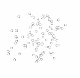
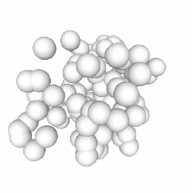
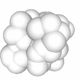
Figure 8: Randomly distributed points decorated with balls of varying radius $r$ – a realization of the Booelean grain model.

For these randomly placed balls the mean volume densities $m_{\mu}$ of the Minkowski functionals are known (e.g.  Mecke and Wagner 1991, Schneider and Weil 1992, also called intensities of Minkowski functionals).

$$\begin{array}[]{llll}m_{0}(A_{r})=&1-{\rm e}^{-\rho M_{0}},&m_{2}(A_{r})=&{\rm e}^{-\rho M_{0}}\ (M_{2}\rho-M_{1}^{2}\rho^{2}),\\[8.61108pt] m_{1}(A_{r})=&{\rm e}^{-\rho M_{0}}\ M_{1}\rho,&m_{3}(A_{r})=&{\rm e}^{-\rho M_{0}}\ (M_{3}\rho-3M_{1}M_{2}\rho^{2}+M_{1}^{3}\rho^{3}),\end{array}$$ (25)

with the number density $\rho$ and

$$M_{0}=\frac{4\pi}{3}r^{3},\quad M_{1}=\frac{\pi}{2}r^{2},\quad M_{2}=\frac{4}{\pi}r,\quad M_{3}=\frac{3}{4\pi}.$$ (26)

Starting from a general point process, decorating it with spheres, we arrive at the germ–grain model (see also Stoyan et al. 1995). The Minkowski functionals or their volume densities calculated for the set $A_{r}$ may be use as tools to describe the underlying point distribution, directly comparable to standard point process statistics like the two–point correlation function (Sect. 3.1) or the nearest neighbor distribution (Sect. 3.4). Indeed, the volume density $m_{0}(A_{r})$ equals the spherical contact distribution or equivalently the void probability minus one: $m_{0}(A_{r})=F(r)=H_{s}(r)=P_{0}(B_{r})-1$ (see also Sect. 3.2). Expressions relating the Minkowski functionals of such a set $A_{r}$, with the $n$–point correlation functions of the underlying point–process may be found in Mecke (1994), Mecke et al. (1994), and Schmalzing et al. (1999b) and the contribution by K. Mecke in this volume.

Already for moderate radii $r$ nearly the whole space is filled with up by $A_{r}$, leading to $m_{0}(A_{r})\approx 1$ and $m_{\mu}(A_{r})\approx 0$, with $\mu>0$. This illustrates the different role the radius $r$ plays for the Minkowski functionals compared to the distance $r$ as used in the two–point correlation function $g(r)$. Already for a fixed radius, the Minkowski functionals of $A_{r}$ are sensitive to the global geometry and topology of $A_{r}$ and, hence, of the decorated point set (see also Sect. 3.3.5). Indeed point sets with an identical two–point correlation function, but with clearly different large scale morphology may be generated easily (see e.g. Baddeley and Silverman 1984, and Szalay 1997).

All galaxy catalogues are spatially limited. To estimate the volume densities of Minkowski functionals for such a realization of the germ–grain model given by the coordinates of galaxies, we use boundary corrections based on principal kinematical formula (see Mecke and Wagner 1991, Stoyan et al. 1995, Schmalzing et al. 1996):

$$m_{\mu}(A_{r})=\frac{M_{\mu}(A_{r}\cap W)}{M_{0}(W)}-\sum_{\nu=0}^{\mu-1}\left(\!\!\!\begin{array}[]{c}{\mu}\\ {\nu}\end{array}\!\!\!\right)m_{\nu}(A_{r})\frac{M_{\mu-\nu}(W)}{M_{0}(W)},$$ (27)

We use the convention $\sum_{n=i}^{j}x_{n}=0$ for $j<i$. An example illustrating these boundary corrections is given in Kerscher et al. (1996a).

In the following an application of these methods to a catalogue of galaxy clusters (Kerscher et al., 1997) (an earlier analysis of a smaller cluster catalogue was already given by Mecke et al. 1994) and to a galaxy catalogue will illustrate the qualitative and quantitative results obtainable with global Minkowski functionals.

3.3.3 Cluster catalogues

The spatial distribution of centers of galaxy clusters, using the Abell/ACO cluster sample of Plionis and Valdarnini (1991), was analyzed with Minkowski functionals applied to the germ–grain model (Kerscher et al., 1997). At first a qualitative discussion of the observed features is presented, followed by a comparison with models for the cluster distribution.

Figure 9: Densities of the Minkowski functionals for the Abell/ACO (solid line) and a Poisson process (shaded area) with the same number density. The shaded area gives the statistical variance of the Poisson process calculated from 100 different realizations.

The most prominent feature of the volume densities of all four Minkowski functionals are the broader extrema for the Abell/ACO data as compared to the results for the Poisson process (see Fig. 9). This is a first indication for enhanced clustering. Let us now look at each functional in detail:
The density of the Minkowski functional $m_{0}$ measures the density of the covered volume. On scales between $25{h^{-1}{\rm Mpc}}$ and $40{h^{-1}{\rm Mpc}}$, $m_{0}$ as a function of $r$ lies slightly below the Poisson data. The volume density is lower because of the clumping of clusters on those scales.
The density of the Minkowski functional $m_{1}$ measures the surface density of the coverage. It has a maximum at about $20{h^{-1}{\rm Mpc}}$ both for the Poisson process and for the cluster data. This maximum is due to the granular structure of the union set on the relevant scales. At the same scales, we find the maximum deviation from the characteristics for the Poisson process. The lower values of $m_{1}$ for the cluster data with respect to the Poisson are again an indication of a significant clumping of clusters at these scales. The functional $m_{1}$ shows also a positive deviation from the Poisson on scales of $(35$…$50){h^{-1}{\rm Mpc}}$ where more coherent structures form in the union set than in the Poisson process, keeping the surface density larger.
The densities of the Minkowski functionals $m_{2}$ and $m_{3}$ characterize in more detail the kind of spatial coverage provided by the union set of balls in the data sample. The density of the total mean curvature $m_{2}$ of the data reaches a maximum at about $10{h^{-1}{\rm Mpc}}$ produced by the dominance of convex (positive $m_{2}$) structures. The density $m_{2}$ at the maximum is reduced with respect to the Poisson process to about 70% (or more than three standard deviations). The integral mean curvature $m_{2}$ has a zero at a scale of $25{h^{-1}{\rm Mpc}}$ (almost the scale of maximum of $m_{1}$) corresponding to the turning–point between structures with mainly convex and concave boundaries (negative $m_{2}$). Significant deviations from the Poisson process occur between this turning point and $40{h^{-1}{\rm Mpc}}$ due to the smaller mean curvature of the union set of the data, probably caused by the interconnection of the void regions in the cluster distribution.
The density of the Euler characteristic $m_{3}$ describes the global topology of the cluster distribution. On small scales all balls are separated. Therefore, each ball gives a contribution of unity to the Euler characteristic and $m_{3}$ is proportional to the cluster number density. As the radius increases, more and more balls overlap and $m_{3}$ decreases. At a scale of about $20{h^{-1}{\rm Mpc}}$ it drops below zero due to the emergence of tunnels in the union set (a double torus has $\chi=-1$). The positive maximum for the Poisson process at scales $\simeq 40{h^{-1}{\rm Mpc}}$ is the signature for the presence of cavities. The nearly linear decrease of the Euler characteristic for the Abell/ACO sample indicates strong clustering on scales $\leq 15{h^{-1}{\rm Mpc}}$. The lack of a significant positive maximum after the minimum shows that only a few cavities form. This suggests a support dimension for the distribution of clusters of less than three. The presence of voids on scales of $30$ to $45{h^{-1}{\rm Mpc}}$ is shown by the enhanced surface area $m_{1}$ and the reduced integral mean curvature $m_{2}$, while on these scales the Euler characteristic $m_{3}$ is approximately zero.

The emphasis of Kerscher et al. (1997) was on the comparison with cosmological model predictions. For this purpose artificial cluster distributions were constructed, from the density field of N–body simulations. Such simulations are still quite costly, and therefore only four specific models were investigated. In Fig. 10 the comparison of the observations with the Standard Cold–Dark–Matter (SCDM) model is shown. This model shows too little clustering on small scales, as it is clearly seen by the enhanced maxima of the surface area $m_{1}$ and the integral mean curvature $m_{2}$, as well as in the flatter decrease of the Euler characteristic $m_{3}$. Additionally, the higher volume $m_{0}$ indicates weak clumping and to few coherent structures also on large scales.

Figure 10: Densities of the Minkowski functionals for the Abell/ACO (solid line in both panels) compared to the SCDM (shaded area in top panel). The shaded area gives 1$\sigma$-error bars of the variance among different realizations.

These deviations may be quantified using some norm for the comparison of the observational data with the model prediction (for details see Kerscher et al. 1997). A comparison of the clusters distribution with CDM–models using the power spectrum (11) lead to a similar conclusions (Retzlaff et al., 1998).

3.3.4 Large fluctuations

A physically interesting point is how well defined are the statistical properties of the galaxy or cluster distribution, determined from one spatially limited realization only. Or in other words, how large are the fluctuations of the morphology for a domain of given size? Kerscher et al. (1998) investigate this using Minkowski functionals, the $J$–function (see section 3.4), and the two–point statistic $\sigma^{2}$ (10).

By normalizing with the functional $M_{\mu}(B_{r})$ of a single ball we can introduce normalized, dimensionless Minkowski functionals $\Phi_{\mu}(A_{r})$,

$$\Phi_{\mu}(A_{r})=\frac{m_{\mu}(A_{r})}{\rho M_{\mu}(B_{r})},$$ (28)

where $\rho$ is the number density. In the case of a Poisson process the exact mean values are known (25). For decorating spheres with radius $r$ one obtains:

$$\begin{array}[]{llll}\Phi_{0}^{P}&=\left(1-{\rm e}^{-\eta}\right)~{}\eta^{-1},&\Phi_{1}^{P}&={\rm e}^{-\eta},\\ \Phi_{2}^{P}&={\rm e}^{-\eta}~{}(1-\tfrac{3\pi^{2}}{32}\eta),&\Phi_{3}^{P}&={\rm e}^{-\eta}~{}(1-3\eta+\tfrac{3\pi^{2}}{32}\eta^{2}),\end{array}$$ (29)

with the dimensionless parameter $\eta=\rho M_{0}(B_{r})=\rho\ 4\pi r^{3}/3$. For $\mu\geq 1$ the measures $\Phi_{\mu}(A_{r})$ contain the exponentially decreasing factor ${\rm e}^{-\eta(r)}$. We employ the reduction

$$\phi_{\mu}(A_{r})=\frac{\Phi_{\mu}(A_{r})}{\Phi_{1}^{P}(A_{r})},\quad\mu\geq 1,$$ (30)

and thereby remove the exponential decay and enhance the visibility of differences in the displays shown below.

We now apply the methods introduced above to explore a redshift catalogue of 5313 IRAS selected galaxies with limiting flux of 1.2 Jy (Fisher et al., 1995). A volume limited sample of 100$h^{-1}$Mpc depth contains 352 galaxies in the northern part, and 358 galaxies in the southern part (with respect to galactic coordinates), as shown in Fig. 6. As far as the number density, i.e. the first moment of the galaxy distribution is concerned, the sample does not reveal significant differences between north and south. However, we want to assess the clustering properties of the data and, above all, tackle the question whether the southern and northern parts differ or not.

Figure 11: Minkowski functionals $\phi_{\mu}$ of a volume limited sample with 100$h^{-1}$Mpc depth extracted from the IRAS 1.2 Jy catalogue; the dark shaded areas represent the southern part, the medium shaded the northern part, and the dotted a Poisson process with the same number density. The shaded areas are the $1\sigma$ errors estimated from twenty realizations for the Poisson process and from twenty errors using a Jackknife procedure with 90% sub–sampling, for the data.

A characterization of the global morphology using the Minkowski functionals (Fig. 11) shows that in both parts of the 1.2 Jy catalogue the clustering of galaxies on scales up to 10$h^{-1}$Mpc is clearly stronger than in the case of a Poisson process, as inferred from the lower values of the functionals for the surface area, $\phi_{1}$, the integral mean curvature, $\phi_{2}$, and the Euler characteristic, $\phi_{3}$. Moreover, the northern and southern parts differ significantly, with the northern part being less clumpy. The most conspicuous features are the enhanced surface area $\phi_{1}$ in the southern part on scales from 12 to 20$h^{-1}$Mpc and the kink in the integral mean curvature $\phi_{2}$ at 14$h^{-1}$Mpc. This behavior indicates that dense substructures in the southern part are filled up at this scale (i.e. the balls in these substructures overlap without leaving holes).

These strongly fluctuating clustering properties are also visible in the $J$–function (Sect. 3.4), and the $\sigma^{2}(B_{r})$ (see (10)). An analysis of possible contaminations and systematic selection effects showed that these fluctuations are real structural differences in the galaxy distribution on scales of 100$h^{-1}$Mpc  even extending to 200$h^{-1}$Mpc  (see also Kerscher et al. 1996b). It is interesting to note that an N–body simulation in a periodic box with side–length of 250$h^{-1}$Mpc (Kolatt et al., 1996) was not able to reproduce these large–scale fluctuations.

3.3.5 Minkowski functionals of excursion sets

In the preceding section the Minkowski functionals were used to characterize the union set of balls, the body $A_{r}$. Consider now a smooth density or temperature field $u({\mathbf{x}})$. We wish to calculate the Minkowski functionals of an excursion set $Q_{\nu}$ over a given threshold $\nu$ (see Fig. 12), defined by

$$Q_{\nu}=\{{\mathbf{x}}~{}|~{}u({\mathbf{x}})\geq\nu\}.$$ (31)

This threshold $\nu$ will be used as a diagnostic parameter.

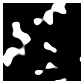
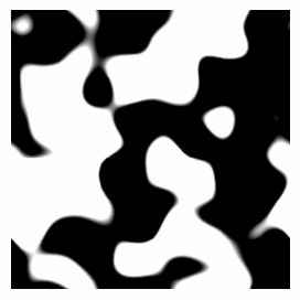
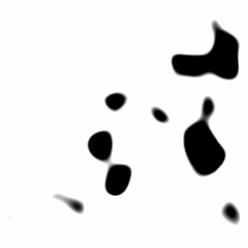
Figure 12: The black set marks the excursion set $Q_{\nu}$ of a Gaussian density field with increasing $\nu$ from left to right. Only the highest peaks remain for large $\nu$.

The geometry and topology of random fields $u({\mathbf{x}})$ and their excursion sets was studied extensively by Adler (1981). Two complementary calculation methods for the Minkowski functionals of the excursion set $Q_{\nu}$ were presented by Schmalzing and Buchert (1997).

Starting with a given point distribution a density field may be constructed with a folding employing some kernel $k_{\epsilon}({\mathbf{z}})$ of width $\epsilon$

$$u({\mathbf{y}})=\sum_{i=1}^{N}\ k_{\epsilon}({\mathbf{x}}_{i}-{\mathbf{y}}).$$ (32)

Often a triangular or a Gaussian kernel sometimes with an adaptive smoothing scale $\epsilon({\mathbf{y}})$ are used. A discussion of smoothing techniques may be found in Silverman (1986).

The Euler characteristic $\chi$ of the excursion set is directly related to the genus $G$ of the iso–density surface separating low from high density regions:

$$G(\partial Q_{\nu})=1-2\chi(Q_{\nu}).$$ (33)

The analysis of cosmological density field using the genus of iso–density surfaces is a well accepted tool in cosmology (see Weinberg et al. 1987, Melott 1990, Coles et al. 1996 and refs. therein), now incorporated in the more general analysis using Minkowski functionals. Especially the Euler characteristic of excursion sets has also applications in other fields like medical image processing (Worsley, 1998).

3.3.6 Gaussianity of the cosmic microwave background

As already mentioned in Sect. 3.2 it is physically very interesting, whether the observed fluctuations in the temperature field of the cosmic microwave background radiation (CMB), as shown in Fig. 1, are compatible with a Gaussian random field model. For a Gaussian random field Tomita (1986) obtained analytical expressions for the Minkowski functionals of $Q_{\nu}$ in arbitrary dimensions. Since the temperature fluctuations are given on the celestial sphere, an adopted integral geometry for spaces with constant curvature must be used (Santaló 1976). Schmalzing and Górski (1998) took this geometric constraint and further complications due to boundary and binning effects, as well as noise contributions into account. They find no significant deviation from a Gaussian random field for the resolution of the COBE data set.

Other methods to test for Gaussianity are based on a wavelet analysis (Hobson et al., 1999) on high–order correlation functions (Heavens, 1999) or on the two–point correlation function of peaks in the temperature fluctuations (Heavens and Sheth, 1999).

3.3.7 Geometry of single objects – shape–finders

Looking at high thresholds $\nu$, the excursion set is mainly composed out of separated regions (see Fig. 12). The morphology of these regions may be characterized using Minkowski functionals and the derived shape–finders (Sahni et al., 1998). Employing the following ratios of the Minkowski functionals $H_{1}=V_{0}/(2V_{1})$, $H_{2}=2V_{1}/(\pi V_{2})$ and $H_{3}=3V_{2}/(4V_{3})$ one may construct the dimensionless shape–finders planarity $P$ and filamentarity $F$

$$P=\frac{H_{2}-H_{1}}{H_{2}+H_{1}}\quad\text{ and }F=\frac{H_{3}-H_{2}}{H_{3}+H_{2}}.$$ (34)

A simple example (Schmalzing et al., 1999a) is provided by a cylinder of radius $r$ and height $\lambda r$ with the Minkowski functionals

$$V_{0}=\pi r^{3}\lambda,\quad V_{1}=\tfrac{\pi}{3}r^{2}(1+\lambda),\quad V_{2}=\tfrac{1}{3}r(\pi+\lambda),\quad V_{3}=1.$$ (35)

The shape–finders planarity $P$ and filamentarity $F$ for this specific example are plotted against each other in Fig. 13. Indeed this is nothing else but an inverted Blaschke diagram for the form factors (Hadwiger 1955, Schneider 1993).

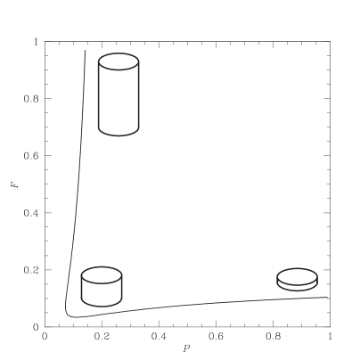
Figure 13: On the left side a plot of the shape–finders for the cylinder with varying $\lambda$ is shown, illustrating the turnover from $\lambda\approx 0$, a plane geometry ($P\approx 1$, $F\ll 1$), through a roughly spherical ($P\approx 0$, $F\approx 0$) to a mainly line like geometry ($P\ll 1$, $F\approx 1$) for $\lambda\gg 1$. On the right side a frequency histogram of the shape–finders determined from the excursion sets of an N–body simulation is shown. Larger circles correspond to more objects within the shape–finder bin (from Schmalzing et al. 1999a).

Following Schmalzing et al. (1999a) the shape–finders may be written in terms of the form factors. With

$$x=\frac{\pi V_{0}V_{2}}{4V_{1}^{2}},\quad y=\frac{8V_{1}V_{3}}{3\pi V_{2}^{2}}$$ (36)

one obtains

$$P=\frac{1-x}{1+x}\quad\text{ and }F=\frac{1-y}{1+y}.$$ (37)

The isoperimetric inequalities (Schneider, 1993) assure that $0\leq P,F\leq 1$ for convex bodies. For a sphere one gets $P=0=F$.

One of the results obtained with the shape–finders applied to single objects in the excursion sets of N–body simulations (Schmalzing et al., 1999a) is given in Fig. 13. This histogram shows that the majority of the regions inside the excursion set has $P\approx 0\approx F$, and a smaller fraction has $P\approx 0$, $F>0$, whereas only a few of the regions have $F\approx 0$ $P>0$. Interpreting regions with e.g. $P\approx 0$, $F>0$ as filamentary or line–like structures is tempting but dangerous, since also non–convex regions are considered. Also, the histogram was constructed from the excursion sets of all thresholds under consideration.

It does not seem to be possible to construct shape–finders based on the global scalar Minkowski functionals facilitating a unique interpretation for non–convex sets. Abandoning the density field approach, and going back to the germ–grain model, and the Minkowski functional of a union set of balls $A_{r}=\bigcup_{i=1}^{N}B_{r}({\mathbf{x}}_{i})$, one may assign a partial Minkowski functional to each ball. These partial Minkowski functionals may be used to extract information on the spatial structure elements – whether the ball around ${\mathbf{x}}_{i}$ is inside a cluster, a sheet or a filament (see Mecke 1994, Platzöder and Buchert 1995, Schmalzing and Diaferio 1999). Another promising global method for extracting shape and symmetry information from non-convex bodies is provided by the global Quermaß vectors (Beisbart et al., 2000).

3.3.8 Other applications of Minkowski functionals

In the preceding applications we analyzed the union set of balls $A_{r}$ or the excursion set $Q_{\nu}$ with Minkowski functionals. Another possibility is to consider Minkowski functionals of the Delauney– or Voronoi–cells, as determined from the corresponding tesselation defined by the given point distribution (Muche 1996, Muche 1997, Kerscher 1998a).

Going beyond motion invariance, instead demanding motion equivariance, one can construct vector–valued extensions of the Minkowski functionals, the Quermaß vectors (Hadwiger and Schneider 1971, Beisbart et al. 1999). Beisbart et al. (2000) investigate the dynamical evolution of the substructure in galaxy clusters using Quermaß vectors (see also Beisbart and Buchert 1998).

3.4 The $J$ function

Other methods to characterize the spatial distribution of points, well known in spatial statistics, are the spherical contact distribution $F(r)$ (also denoted by $H_{s}(r)$), i.e. the distribution function of the distances $r$ between an arbitrary point and the nearest object in the point set $X$, and the nearest neighbor distance distribution $G(r)$, that is defined as the distribution function of distance $r$ of an object in $X$ to the nearest other object in $X$. $F(r)$ is related to the void probability $P_{0}(B_{r})$ by $F(r)=1-P_{0}(B_{r})$. For a Poisson distribution it is simply

$$G(r)=F(r)=1-\exp\left(-\rho\frac{4\pi}{3}r^{3}\right).$$ (38)

Recently, van Lieshout and Baddeley (1996) suggested to use the ratio

$$J(r)=\frac{1-G(r)}{1-F(r)}$$ (39)

as a further distributional characteristic. For a Poisson distribution $J(r)=1$ follows directly from (38). As shown by van Lieshout and Baddeley (1996), a clustered point distribution implies $J(r)\leq 1$, whereas regular structures are indicated by $J(r)\geq 1$. However, Bedford and van den Berg (1997) showed that $J=1$ does not imply a Poisson process. For several point process models $J(r)$, or at least limiting values for $J(r)$, are known (van Lieshout and Baddeley, 1996). The $J$ function was considered by White (1979) as the “first conditional correlation function” and used by Sharp (1981) to test hierarchical models. The relation between $J(r)$ and the cumulants $\xi_{n}(r)$ was used by Kerscher (1998b). An empirical study of the performance of the $J$–function for several point process models is given by Thönnes and van Lieshout (1999). A refined definition of the $J$-function “without edge correction” may be especially useful for a test on spatial randomness (Baddeley et al., 1999).

3.4.1 Clustering of galaxies

The $J$–function may be used to characterize the distribution of galaxies or galaxy clusters and for the comparison with the results from simulations, similar to the application of the Minkowski functionals in sect. 3.3.3. This approach was pursued by Kerscher et al. (1999a). The Perseus–Pisces redshift survey (Wegner et al. 1993 and refs. therein) was compared with galaxy samples constructed from a mixed dark matter simulation. The observed $J(r)$ determined from a volume limited sample with 79$h^{-1}$Mpc  depth differs significantly from the results of the simulations (Fig. 14). Especially on small scales the galaxy distribution shows a stronger clustering, as seen by steeper decreasing $J(r)$.

Figure 14: $J(r)$ for the volume limited sample from Perseus–Pisces redshift survey (solid line) and the 1$\sigma$ range determined from galaxy samples generated by a mixed dark matter simulation.

We also could show that modeling the galaxy distribution with a simple Poisson cluster process is not appropriate.

3.4.2 Regularity in the distribution of super–clusters?

Einasto et al. (1997b) report a peak in the 3D–power spectrum (the Fourier transform of $\xi_{2}$) of a catalogue of clusters on a scale of 120$h^{-1}$Mpc. Broadhurst et al. (1990) observed periodicity on approximately the same scale in an analysis of 1D–data from a pencil–beam redshift survey. As is well known from the theory of fluids, the regular distribution (e.g. of molecules in a hard–core fluid) reveals itself in an oscillating two–point correlation function and a peak in the structure function respectively (see e.g. Hansen and McDonnald 1986, and the contribution of H. Löwen in this volume). In accordance with this an oscillating two–point correlation function $\xi_{2}(r)$ or at least a first peak was reported on approximately the same scale (e.g. Mo et al. 1992 and Einasto et al. 1997a). The existence of regularity on large scales implies a preferred scale in the initial conditions, which would be of major physical interest.

Using the $J(r)$–function Kerscher (1998b) investigates the super–cluster catalogue (Einasto et al., 1997c) constructed from an earlier version of the cluster catalogue by Andernach and Tago (1998) using a friend–of–friends procedure. (The friend–of–friends procedure is called single linkage clustering in the mathematical literature). Comparing with Poisson distributed points one clearly recognizes that the super–cluster catalogue is a regular point distribution (Fig. 15).

Figure 15: $J(r)$ determined from the super–cluster sample (solid line) is shown together with the 1–$\sigma$ range determined from a pure Poisson process (dotted area) and a Poisson process followed by a similar friend–of–friends procedure (dashed area) as used to construct the super–cluster catalogue.

However, a similar signal for $J(r)$ may be obtained by starting with a Poisson process followed by a friend–of–friends procedure with the same linking length as used in the construction of the super–cluster catalogue. Only some indication for a regular distribution on large scales remains, showing that this super–cluster catalogue is seriously affected by the construction method.

3.4.3 $G_{n}$ and $F_{n}$

As a direct generalization of the nearest neighbor distance distribution one may consider the $n$–th neighbor distance distributions $G_{n}(r)$, the distribution of the distance $r$ to the $n$–th nearest point (e.g.  Stoyan and Stoyan 1994). For a Poisson process in three dimensions we have

$$G_{n}(r)=1-\frac{\Gamma\left(n,\rho\frac{4\pi}{3}r^{3}\right)}{\Gamma(n)},$$ (40)

shown in Fig. 16. $\Gamma(n,x)=\int_{x}^{\infty}{\rm d}{s}\ s^{n-1}e^{-s}$ is the incomplete Gamma–function, $\Gamma(n)=\Gamma(n,0)$ the complete. Clearly $G_{1}(r)=G(r)$. In Fig. 16 the curves for the first five $G_{n}(r)$ for a Poisson process are shown, together with their densities $p_{n}(r)$ defined by

$$G_{n}(r)=\int_{0}^{r}{\rm d}s\ p_{n}(s).$$ (41)

The sum of these densities is directly related to the two–point correlation function (Mazur, 1992)

$$g(r)\ \rho\ 4\pi r^{2}=\sum_{n=1}^{\infty}\ p_{n}(r).$$ (42)

Figure 16: In the left plot you see the $G_{n}(r)$ with $n=1,\dots,5$ for a Poisson process with $\rho=100$. In the right plot the corresponding densities $p_{n}(r)$ are shown.

The $n$–th spherical contact distribution $F_{n}(r)$ is the distribution function of the distances $r$ between an arbitrary point and the $n$–th closest object in the point set $X$ (we assume that the $n$–th closest point is unique). Clearly $F_{1}(r)=F(r)$. For stationary and isotropic point processes $F_{n}(r)$ is the probability to find at least $n$ points inside a sphere $B_{r}$ with radius $r$, and therefore

$$F_{n}(r)=\sum_{i=n}^{\infty}P_{i}(B_{r})=1-\sum_{i=0}^{n-1}P_{i}(B_{r}),$$ (43)

where $P_{i}(B_{r})$ are the counts–in–cells as discussed in Sect. 3.2.

For a Poisson process with number density $\rho$ we obtain directly from (14)

$$F_{n}(r)=1-\exp(-\rho|B_{r}|)\sum_{i=0}^{n-1}\frac{(\rho|B_{r}|)^{i}}{i!},$$ (44)

which is essentially the series expansion of the incomplete gamma function (see e.g. Abramowitz and Stegun 1984). Therefore,

$$F_{n}(r)=1-\frac{\Gamma\left(n,\rho\frac{4\pi}{3}r^{3}\right)}{\Gamma(n)},$$ (45)

and we explicitely see that for a Poisson process

$$F_{n}(r)=G_{n}(r)$$ (46)

This is a special case of the “Slivnyak’s theorem” (Stoyan et al., 1995).

A very interesting feature of the $G_{n}(r)$ and $F_{n}(r)$ is their sensitivity to structures on large scales increasing with $n$. As an illustration consider the interval $\Delta_{n}\subset{\mathbb{R}}^{+}$ specified by $\int_{\Delta_{n}}{\rm d}s\ p_{n}(s)=0.9$. Then $\Delta_{n}$ is the interval in which 90% of the distances to the $n$–th neighbor lie. (The choice of 0.9 is arbitrary and may certainly be adopted to the problem considered. Also the interval $\Delta_{n}$ is “centered” as shown in Fig. 16.) The empirical $G_{n}(r)$ may be used to probe structures within this specific radial range as illustrated in Fig. 16. Going to larger $n$ one considers distance intervals for larger radii.

3.4.4 The $J_{n}$ function

A drawback of the $J(r)$–function in empirical investigations is that it becomes ill defined for large radii, since the empirical $F(r)$ reaches unity and the quotient in (39) diverges. In the following we will discuss the straightforward generalization of the $J$–function (39), introducing the $J_{n}(r)$ functions:

$$J_{n}(r)=\frac{1-G_{n}(r)}{1-F_{n}(r)}.$$ (47)

From (46) we obtain directly for a Poisson process

$$J_{n}(r)=1\quad\text{ for all $n$}.$$ (48)

Qualitatively we expect the same behavior of the $J_{n}(r)$–functions as for the $J(r)$–function, but now for a radius $r$ in the interval $\Delta_{n}$ (defined at the end of Sect. 3.4.3).

• If a point distribution shows clustering on scales $r$ in $\Delta_{n}$, the $G_{n}(r)$ increases faster than for a Poisson process since the $n$–th nearest neighbor is typically closer. $F_{n}(r)$ increases more slowly than for a random distribution. Both effects result in a $J_{n}(r)\leq 1$.

• On the other hand, for a point distribution regular on the scale $r$ in $\Delta_{n}$, $G_{n}(r)$ increases more slowly than for a Poisson process, since the $n$–th neighbor is found at a finite characteristic distance. $F_{n}(r)$ increases stronger since the distance from a random point to the $n$–th closest point on the regular structure is typically smaller. This results in $J_{n}(r)\geq 1$.

• $J_{n}(r)=1$ indicates the transition from regular to clustered structures on scales $r$ in $\Delta_{n}$.

With a simple point process model we illustrate these properties. In a Matérn cluster process a single cluster consists out of $\mu$ points in the mean, randomly distributed inside a sphere of radius $R$, where the number of points follows a Poisson distribution. The clusters centers (not belonging to the point process) form a Poisson process with a density of $\rho/\mu$ (Stoyan et al., 1995). In Fig. 17 the strong clustering in the Matérn cluster process is visible from a decline of the $J_{n}(r)$. This decline becomes weaker with increasing $n$. For large radii $r$ the $J_{n}$ acquire a constant value. Investigating larger scales, i.e. for large $n$, the constant value of $J_{n}$ shows a trend towards unity, i.e. we start to “see” the Poisson distribution of the clusters centers.

Figure 17: The $J_{n}(r)$ with $n=1,\ldots 10$ (bending up successively) for a Matérn cluster process with $\mu=10$ and $R=1.5{h^{-1}{\rm Mpc}}$ calculated using the reduced sample estimators.

3.4.5 On our way to large scales

A similar behavior may be identified in the galaxy distribution. We calculate the $J_{n}$–functions for a volume limited sample of galaxies extracted from the IRAS 1.2 Jy catalogue with 200$h^{-1}$Mpc  depth using the reduced sample estimator for both $F_{n}$ and $G_{n}$. For small $n$, i.e.  small scales, the $J_{n}(r)$ are all smaller than unity, indicating clustering out to scales of 40$h^{-1}$Mpc(see Fig. 18). For large $n$ the $J_{n}$ are consistent with no clustering, i.e. $J_{n}=1$. However a trend towards a $J_{n}$ larger than unity, indicating regularity is observed. Clearly, the results obtained from this sparse sample with 280 galaxies only may serve mainly as an illustration of the method – to obtain decisive results we will have to wait for deeper surveys.

Figure 18: In the left plot the $J_{n}$ of the IRAS galaxies are shown with $n=1,4,7$ (solid, dotted, dashed), in the right plot the $J_{n}$ with $n=10,15,20$ (solid, dotted, dashed).

4 Summary and Outlook

In Sections 3.3.3 and 3.4.1 we discussed that advanced geometrical methods like the Minkowski functionals and the $J$–function are able to constrain parameters of cosmological models. However, these geometric methods are not only limited to the parameter estimation in cosmological simulations, they are also valuable tools as point process statistics in general. The direct probe of galaxy surveys with geometrical methods showed that the large–scale structure exhibits strong morphological fluctuations (Sect. 3.3.4). Such fluctuations are often attributed to “cosmic variance” in an Universe homogeneous on very large scales. However the fluctuations are astonishingly large even on scales of 200$h^{-1}$Mpc. A preferred scale, may be viewed as an indication for a homogeneous galaxy distribution on large scales. Especially geometric methods like the $J$– and $J_{n}$–functions may be helpful to identify a preferred scale in the galaxy distribution.

Perspectives for future research might be as follows:
Starting with the Minkowski functionals or other well founded geometrical tools, more specialized methods may be constructed to understand certain features in the galaxy distribution in detail. An example are the vector valued extension of the Minkowski functionals, the Quermaß–vector, used in the investigation of the substructure in galaxy clusters.
In empirical work, one has to determine these geometrical measures from a given point set. The construction of estimators with well understood distributional properties is crucial to be able to draw decisive conclusions from the data.
Using these geometrical methods as tools for constraining the cosmological parameters will be one way to go. Currently this is mainly performed by comparisons with N–body simulations. Clearly a more direct link between the geometry and the dynamics of matter in the Universe promoting our understanding how structures form is desirable. Carefully constructed approximations may be the key ingredient.
Another way in trying to understand structure formation is to directly investigate the appearance of geometric features like walls, filaments, and clusters – or to identify a preferred scale showing up in a regular distribution on large scales. Such findings will guide us in the construction of approximations, which are able to reproduce such geometric features.

One may find some of the more recent articles on the preprint servers
http://xxx.lanl.gov/archive/astro-ph or
http://xxx.lanl.gov/archive/gr-qc.
Numbers like astro-ph/9710207 refer to preprints on these servers. An abstract server for articles appaering in several astrophysical journals is
http://ads.harvard.edu/.
Articles older than a few years are scanned and and may be donloaded from there.

References

- Abramowitz and Stegun (1984) Abramowitz, M. X. and Stegun, I. A. (1984): Pocketbook of Mathematical Functions. Harri Deutsch, Thun, Frankfurt/Main.
- Adler (1981) Adler, R. J. (1981): The geometry of random fields. John Wiley & Sons, Chichester.
- Andernach and Tago (1998) Andernach, H. and Tago, E. (1998): Current status of the ACO cluster redshift compilation. In V. Müller, S. Gottlöber, J. P. Mücket, and J. Wambsgans, eds., Proc. of the 12th Potsdam Cosmology Workshop 1997, Large Scale Structure: Tracks and Traces. World Scientific, Singapore. Astro-ph/9710265.
- Baddeley et al. (1999) Baddeley, A. J., Kerscher, M., Schladitz, K., and Scott, B. (1999): Estimating the function without edge correction. Statist. Neerlandica, in press .
- Baddeley and Silverman (1984) Baddeley, A. J. and Silverman, B. W. (1984): A cautionary example on the use of second–order methods for analyzing point patterns. Biometrics, 40, 1089–1093.
- Balian and Schaeffer (1989) Balian, R. and Schaeffer, R. (1989): Scale–invariant matter distribution in the Universe I. counts in cells. Astron. Astrophys., 220, 1–29.
- Bardeen et al. (1986) Bardeen, J. M., Bond, J. R., Kaiser, N., and Szalay, A. S. (1986): The statistics of peaks of Gaussian random fields. Ap. J., 304, 15–61.
- Barrow et al. (1985) Barrow, J. D., Sonoda, D. H., and Bhavsar, S. P. (1985): Minimal spanning trees, filaments and galaxy clustering. Mon. Not. Roy. Astron. Soc., 216, 17–35.
- Bedford and van den Berg (1997) Bedford, T. and van den Berg, J. (1997): A remark on the van Lieshout and Baddeley J–function for point processes. Adv. Appl. Prob., 29, 19–25.
- Beisbart and Buchert (1998) Beisbart, C. and Buchert, T. (1998): Characterizing cluster morphology using vector–valued minkowski functionals. In V. Müller, S. Gottlöber, J. P. Mücket, and J. Wambsgans, eds., Proc. of the 12th Potsdam Cosmology Workshop 1997, Large Scale Structure: Tracks and Traces. World Scientific, Singapore. astro-ph/9711034 .
- Beisbart et al. (2000) Beisbart, C., Buchert, T., Bartelmann, M., Colberg, J. G., and Wagner, H. (2000): Morphological evolution of galaxy clusters: First application of the quermaß vectors. in preparation .
- Beisbart et al. (1999) Beisbart, C., Buchert, T., and Wagner, H. (1999): Morphometry of galaxy clusters. submitted .
- Bernardeau and Kofman (1995) Bernardeau, F. and Kofman, L. (1995): Properties of the cosmological density distribution function. Ap. J., 443, 479–498.
- Bertschinger (1992) Bertschinger, E. (1992): Large-scale structures and motions: Linear theory and statistics. In V. Martinez, M. Portilla, and D. Saez, eds., New Insights into the Universe, number 408 in Lecture Notes in Physics , pages 65–126. Springer Verlag, Berlin.
- Borgani (1995) Borgani, S. (1995): Scaling in the universe. Physics Rep., 251, 1–152.
- Börner (1993) Börner, G. (1993): The Early Universe, Facts and Fiction. Springer Verlag, Berlin, 3rd edition.
- Bouchet et al. (1992) Bouchet, F. R., Juszkiewicz, R., Colombi, S., and Pellat, R. (1992): Weakly nonlinear gravitational instability for arbitrary Omega. Ap. J. Lett., 394, L5–L8.
- Broadhurst et al. (1990) Broadhurst, T. J., Ellis, R. S., Koo, D. C., and Szalay, A. S. (1990): Large–scale distribution of galaxies at the galactic poles. Nature, 343, 726.
- Buchert (1996) Buchert, T. (1996): Lagrangian perturbation approach to the formation of large–scale structure. In S. Bonometto, J. Primack, and A. Provenzale, eds., Proceedings of the international school of physics Enrico Fermi. Course CXXXII: Dark matter in the Universe. Società Italiana di Fisica, Varenna sul Lago di Como.
- Buchert (1999) Buchert, T. (1999): On average properties of inhomogeneous fluids in general relativity: I. dust cosmologies. G.R.G. in press, gr-qc/9906015.
- Buchert and Ehlers (1997) Buchert, T. and Ehlers, J. (1997): Averaging inhomogeneous Newtonian cosmologies. Astron. Astrophys., 320, 1–7.
- Cappi et al. (1998) Cappi, A., Benoist, C., Da Costa, L., and Maurogordato, S. (1998): Is the universe a fractal? results from the SSRS2. Astron. Astrophys., 335, 779–788.
- Coles et al. (1996) Coles, P., Davies, A., and Pearson, R. C. (1996): Quantifying the topology of large–scale structure. Mon. Not. Roy. Astron. Soc., 281, 1375–1384.
- Coles and Lucchin (1994) Coles, P. and Lucchin, F. (1994): Cosmology: The origin and evolution of cosmic structure. John Wiley & Sons, Chichester.
- Colombi et al. (1998) Colombi, S., Szapudi, I., and Szalay, A. S. (1998): Effects of sampling on statistics of large scale structure. Mon. Not. Roy. Astron. Soc., 296, 253.
- da Costa et al. (1998) da Costa, L. N., Willmer, C. N. A., Pellegrini, P., Chaves, O. L., Rite, C., Maia, M. A. G., Geller, M. J., Latham, D. W., Kurtz, M. J., Huchra, J. P., Ramella, M., Fairall, A. P., Smith, C., and Lipari, S. (1998): The Southern Sky Redshift Survey. A. J., 116, 1–7.
- Daley and Vere-Jones (1988) Daley, D. J. and Vere-Jones, D. (1988): An Introduction to the Theory of Point Processes. Springer Verlag, Berlin.
- Dolgov et al. (1999) Dolgov, A., Doroshkevich, A., Novikov, D., and Novikov, I. (1999): Geometry and statistics of cosmic microwave polarization. Astro-ph/9901399.
- Doroshkevich et al. (1999) Doroshkevich, A. G., , Müller, V., Retzlaff, J., and Turchaninov, V. (1999): Superlarge–scale structure in n–body simulations. Mon. Not. Roy. Astron. Soc., 306, 575–591.
- Efstathiou (1996) Efstathiou, G. (1996): Observations of large–scale structure in the Universe. In R. Schaeffer, J. Silk, M. Spiro, and J. Zinn-Justin, eds., LesHouches Session LX: cosmology and large scale structure, august 1993, pages 133–252. Elsevier, Amsterdam.
- Einasto et al. (1997a) Einasto, J., Einasto, M., Frisch, P., Gottlöber, S., Müller, V., Saar, V., Starobinsky, A. A., Tago, E., and Andernach, D. T. H. (1997a): The supercluster–void network. II. an oscillating cluster correlation function. Mon. Not. Roy. Astron. Soc., 289, 801–812.
- Einasto et al. (1997b) Einasto, J., Einasto, M., Gottlöber, S., Müller, V., Saar, V., Starobinsky, A. A., Tago, E., Tucker, D., Andernach, H., and Frisch, P. (1997b): A 120-Mpc periodicity in the three–dimensional distribution of galaxy superclusters. Nature, 385, 139–141.
- Einasto et al. (1997c) Einasto, M., Tago, E., Jaaniste, J., Einasto, J., and Andernach, H. (1997c): The supercluster–void network. I. the supercluster catalogue and large–scale distribution. Astron. Astrophys. Suppl., 123, 119.
- Fiksel (1988) Fiksel, T. (1988): Edge–corrected density estimators for point processes. Statistics, 19, 67–75.
- Fisher et al. (1995) Fisher, K. B., Huchra, J. P., Strauss, M. A., Davis, M., Yahil, A., and Schlegel, D. (1995): The IRAS 1.2 Jy survey: Redshift data. Ap. J. Suppl., 100, 69.
- Gaite et al. (1999) Gaite, J., Dominguez, A., and Perez-Mercader, J. (1999): The fractal distribution of galaxies and the transition to homogeneity. Ap. J., 522, L5–L8.
- Goldenfeld (1992) Goldenfeld, N. (1992): Lectures on Phase Transitions and the Renormalization Group. Addison–Wesley, Reading, MA.
- Grassberger and Procaccia (1984) Grassberger, P. and Procaccia, I. (1984): Dimensions and entropies of strange attractors from fluctuating dynamics approach. Physica D, 13, 34–54.
- Gunn (1995) Gunn, J. E. (1995): The Sloan Digital Sky Survey. Bull. American Astron. Soc., 186, 875.
- Hadwiger (1955) Hadwiger, H. (1955): Altes und Neues über konvexe Körper. Birkhäuser, Basel.
- Hadwiger (1957) Hadwiger, H. (1957): Vorlesungen über Inhalt, Oberfläche und Isoperimetrie. Springer Verlag, Berlin.
- Hadwiger and Schneider (1971) Hadwiger, H. and Schneider, R. (1971): Vektorielle Integralgeometrie. Elemente der Mathematik, 26, 49–72.
- Hamilton (1993) Hamilton, A. J. S. (1993): Toward better ways to measure the galaxy correlation function. Ap. J., 417, 19–35.
- Hansen and McDonnald (1986) Hansen, J. P. and McDonnald, I. R. (1986): Theory of Simple Liquids. Academic Press, New York and London.
- Heavens (1999) Heavens, A. F. (1999): Estimating non–Gaussianity in the microwave background. Mon. Not. Roy. Astron. Soc., 299, 805–808.
- Heavens and Sheth (1999) Heavens, A. F. and Sheth, R. K. (1999): The correlation of peaks in the microwave background. submitted, astro-ph/9906301 .
- Hobson et al. (1999) Hobson, M. P., Jones, A. W., and Lasenby, A. N. (1999): Wavelet analysis and the detection of non–Gaussianity in the CMB. Mon. Not. Roy. Astron. Soc., 309, 125–140.
- Huchra et al. (1995) Huchra, J. P., Geller, M. J., and Corwin Jr., H. G. (1995): The CfA redshift survey: Data for the NGP + 36 zone. Ap. J. Suppl., 99, 391.
- Huchra et al. (1990) Huchra, J. P., Geller, M. J., De Lapparent, V., and Corwin Jr., H. G. (1990): The CfA redshift survey – data for the NGP + 30 zone. Ap. J. Suppl., 72, 433–470.
- Jing and Börner (1998) Jing, Y. P. and Börner, G. (1998): The three–point correlation function of galaxies. Ap. J., 503, 37.
- Juszkiewicz et al. (1995) Juszkiewicz, R., Weinberg, D. H., Amsterfamski, P., Chodorowski, M., and Bouchet, F. R. (1995): Weakly nonlinear Gaussian fluctuations and the Edgeworth expansion. Ap. J., 442, 39–56.
- Kates et al. (1991) Kates, R., Kotok, E., and Klypin, A. (1991): High–resolution simulations of galaxy formation in a cold dark matter scenario. Astron. Astrophys., 243, 295–308.
- Kauffmann et al. (1997) Kauffmann, G., Nusser, A., and Steinmetz, M. (1997): Galaxy formation and large-scale bias. Mon. Not. Roy. Astron. Soc., 286, 795–811.
- Kerscher (1998a) Kerscher, M. (1998a): Morphologie großräumiger Strukturen im Universum. GCA–Verlag, Herdecke.
- Kerscher (1998b) Kerscher, M. (1998b): Regularity in the distribution of superclusters? Astron. Astrophys., 336, 29–34.
- Kerscher (1999) Kerscher, M. (1999): The geometry of second–order statistics – biases in common estimators. Astron. Astrophys., 343, 333–347.
- Kerscher et al. (1999a) Kerscher, M., Pons-Bordería, M. J., Schmalzing, J., Trasarti-Battistoni, R., Martínez, V. J., Buchert, T., and Valdarnini, R. (1999a): A global descriptor of spatial pattern interaction in the galaxy distribution. Ap. J., 513, 543–548.
- Kerscher et al. (1996a) Kerscher, M., Schmalzing, J., and Buchert, T. (1996a): Analyzing galaxy catalogues with Minkowski functionals. In P. Coles, V. Martínez, and M. J. Pons Bordería, eds., Mapping, measuring and modelling the Universe, pages 247–252. Astronomical Society of the Pacific, Valencia.
- Kerscher et al. (1996b) Kerscher, M., Schmalzing, J., Buchert, T., and Wagner, H. (1996b): The significance of the fluctuations in the IRAS 1.2 Jy galaxy catalogue. In R. Bender, T. Buchert, and P. Schneider, eds., Proc. SFB workshop on Astro–particle physics Ringberg 1996, Report SFB375/P002, pages 83–98. Ringberg, Tegernsee.
- Kerscher et al. (1998) Kerscher, M., Schmalzing, J., Buchert, T., and Wagner, H. (1998): Fluctuations in the 1.2 Jy galaxy catalogue. Astron. Astrophys., 333, 1–12.
- Kerscher et al. (1997) Kerscher, M., Schmalzing, J., Retzlaff, J., Borgani, S., Buchert, T., Gottlöber, S., Müller, V., Plionis, M., and Wagner, H. (1997): Minkowski functionals of Abell/ACO clusters. Mon. Not. Roy. Astron. Soc., 284, 73–84.
- Kerscher et al. (1999b) Kerscher, M., Szapudi, I., and Szalay, A. (1999b): A comparison of estimators for the two-point correlation function: dispelling the myths. submitted .
- Klain and Rota (1997) Klain, D. A. and Rota, C.-C. (1997): Introduction to Geometric Probability. Cambridge University Press, Cambridge.
- Kolatt et al. (1996) Kolatt, T., Dekel, A., Ganon, G., and Willick, J. A. (1996): Simulating our cosmological neighborhood: Mock catalogs for velocity analysis. Ap. J., 458, 419–434.
- Landy and Szalay (1993) Landy, S. D. and Szalay, A. S. (1993): Bias and variance of angular correlation functions. Ap. J., 412, 64–71.
- Maddox (1998) Maddox, S. (1998): The 2df galaxy redshift survey: Preliminary results. In V. Müller, S. Gottlöber, J. P. Mücket, and J. Wambsgans, eds., Proc. of the 12th Potsdam Cosmology Workshop 1997, Large Scale Structure: Tracks and Traces. World Scientific, Singapore. Astro-ph/9711015.
- Mandelbrot (1982) Mandelbrot, B. (1982): The Fractal Geometry of Nature. Freeman, San Francisco.
- Martínez (1996) Martínez, V. J. (1996): Measures of galaxy clustering. In S. Bonometto, J. Primack, and A. Provenzale, eds., Proceedings of the international school of physics Enrico Fermi. Course CXXXII: Dark matter in the Universe. Società Italiana di Fisica, Varenna sul Lago di Como.
- Matheron (1989) Matheron, G. (1989): Estimating and Choosing: An Essay on Probability in Practice. Springer Verlag, Berlin.
- Mazur (1992) Mazur, S. (1992): Neighborship partition of the radial distribution function for simple liquids. J. Chem. Phys., 97, 9276–9282.
- McCauley (1997) McCauley, J. L. (1997): Are galaxy distributions scale invariant? a perspective from dynamical systems theory. submitted, astro-ph/9703046 .
- McCauley (1998) McCauley, J. L. (1998): The galaxy distributions: Homogeneous, fractal, or neither? Fractals, 6, 109–119.
- Mecke (1994) Mecke, K. R. (1994): Integralgeometrie in der Statistischen Physik: Perkolation, komplexe Flüssigkeiten und die Struktur des Universums. Harri Deutsch, Thun, Frankfurt/Main.
- Mecke et al. (1994) Mecke, K. R., Buchert, T., and Wagner, H. (1994): Robust morphological measures for large–scale structure in the Universe. Astron. Astrophys., 288, 697–704.
- Mecke and Wagner (1991) Mecke, K. R. and Wagner, H. (1991): Euler characteristic and related measures for random geometric sets. J. Stat. Phys., 64, 843.
- Melott (1990) Melott, A. L. (1990): The topology of large–scale structure in the Universe. Physics Rep., 193, 1–39.
- Milne and Westcott (1972) Milne, R. K. and Westcott, M. (1972): Further results for Gauss–poisson processes. Adv. Appl. Prob., 4, 151–176.
- Mo et al. (1992) Mo, H. J., Deng, Z. G., Xia, X. Y., Schiller, P., and Börner, G. (1992): Typical scales in the distribution of galaxies and clusters of galaxies from unnormalized pair counts. Astron. Astrophys., 257, 1–10.
- Muche (1996) Muche, L. (1996): Distributional properties of the three–dimensional Poisson Delauney cell. J. Stat. Phys., 84, 147–167.
- Muche (1997) Muche, L. (1997): Fragmenting the universe and the Voronoi tesselation. preprint, Freiberg 1997 .
- Novikov et al. (1999) Novikov, D., Feldman, H. A., and Shandarin, S. F. (1999): Minkowski functionals and cluster analysis for CMB maps. Int. J. Mod. Phys., D8, 291–306.
- Padmanabhan (1993) Padmanabhan, T. (1993): Structure formation in the Universe. Cambridge University Press, Cambridge.
- Padmanabhan and Subramanian (1993) Padmanabhan, T. and Subramanian, K. (1993): Zel’dovich approximation and the probability distribution for the smoothed density field in the nonlinear regime. Ap. J., 410, 482–487.
- Peacock (1992) Peacock, J. A. (1992): Satistics of cosmological density fields. In V. Martinez, M. Portilla, and D. Saez, eds., New Insights into the Universe, number 408 in Lecture Notes in Physics , pages 65–126. Springer Verlag, Berlin.
- Peebles (1973) Peebles, P. (1973): Satistical analysis of catalogs of extragalactic objects. I. theory. Ap. J., 185, 413–440.
- Peebles (1980) Peebles, P. J. E. (1980): The Large Scale Structure of the Universe. Princeton University Press, Princeton, New Jersey.
- Platzöder and Buchert (1995) Platzöder, M. and Buchert, T. (1995): Applications of Minkowski functionals for the statistical analysis of dark matter models. In A. Weiss, G. Raffelt, W. Hillebrandt, and F. von Feilitzsch, eds., Proc. of “1st SFB workshop on Astro-particle physics”, Ringberg, Tegernsee, pages 251–263. astro-ph/9509014 .
- Plionis and Valdarnini (1991) Plionis, M. and Valdarnini, R. (1991): Evidence for large–scale structure on scales about 300/h Mpc. Mon. Not. Roy. Astron. Soc., 249, 46–62.
- Pons–Bordería et al. (1999) Pons–Bordería, M.-J., Martínez, V. J., Stoyan, D., Stoyan, H., and Saar, E. (1999): Comparing estimators of the galaxy correlation function. Ap. J., 523, 480.
- Retzlaff et al. (1998) Retzlaff, J., Borgani, S., Gottlöber, S., Klypin, A., and Müller, V. (1998): Constraining cosmological models with cluster power spectra. New Astronomy, 3, 631–646.
- Sahni et al. (1997) Sahni, V., Sathyaprakash, B. S., and Shandarin, S. F. (1997): Probing large-scale structure using percolation and genus curves. Ap. J., 476, L1–L5.
- Sahni et al. (1998) Sahni, V., Sathyaprakash, B. S., and Shandarin, S. F. (1998): Shapefinders: A new shape diagnostic for large–scale structure. Ap. J., 495, L5–L8.
- Sandage (1995) Sandage, A. (1995): Practical cosmology: Inventing the past. In A. Sandage, R. Kron, and M. Longair, eds., The Deep Universe, Saas–Fee Advanced Course Lecture Notes 1993, pages 1–232. Swiss society for Astrophysics and Astronomy, Springer Verlag, Berlin.
- Santaló (1976) Santaló, L. A. (1976): Integral Geometry and Geometric Probability. Addison–Wesley, Reading, MA.
- Sathyaprakash et al. (1998a) Sathyaprakash, B. S., Sahni, V., and Shandarin, S. F. (1998a): Morphology of clusters and superclusters in N-body simulations of cosmological gravitational clustering. Ap. J., 508, 551–569.
- Sathyaprakash et al. (1998b) Sathyaprakash, B. S., Sahni, V., Shandarin, S. F., and Fisher, K. B. (1998b): Filaments and pancakes in the IRAS 1.2 Jy redshift survey. Ap. J., 507, L109–L112.
- Schmalzing and Buchert (1997) Schmalzing, J. and Buchert, T. (1997): Beyond genus statistics: A unifying approach to the morphology of cosmic structure. Ap. J. Lett., 482, L1–L4.
- Schmalzing et al. (1999a) Schmalzing, J., Buchert, T., Melott, A., Sahni, V., Sathyaprakash, B., and Shandarin, S. (1999a): Disentangling the cosmic web I: Morphology of isodensity contours. in press, astro-ph/9904384 .
- Schmalzing and Diaferio (1999) Schmalzing, J. and Diaferio, A. (1999): Topology and geometry of the CfA2 redshift survey. in press, astro-ph/9910228 .
- Schmalzing and Górski (1998) Schmalzing, J. and Górski, K. M. (1998): Minkowski functionals used in the morphological analysis of cosmic microwave background anisotropy maps. Mon. Not. Roy. Astron. Soc., 297, 355–365.
- Schmalzing et al. (1999b) Schmalzing, J., Gottlöber, S., Kravtsov, A., and Klypin, A. (1999b): Quantifying the evolution of higher order clustering. Mon. Not. Roy. Astron. Soc., 309, 1007–1016.
- Schmalzing et al. (1996) Schmalzing, J., Kerscher, M., and Buchert, T. (1996): Minkowski functionals in cosmology. In S. Bonometto, J. Primack, and A. Provenzale, eds., Proceedings of the international school of physics Enrico Fermi. Course CXXXII: Dark matter in the Universe, pages 281–291. Società Italiana di Fisica, Varenna sul Lago di Como.
- Schneider (1993) Schneider, R. (1993): Convex bodies: the Brunn–Minkowski theory. Cambridge University Press, Cambridge.
- Schneider and Weil (1992) Schneider, R. and Weil, W. (1992): Integralgeometrie. Bernd G. Teubner, Leipzig, Berlin.
- Shandarin (1983) Shandarin, S. F. (1983): Percolation theory and the cell–lattice structure of the Universe. Sov. Astron. Lett., 9, 104–106.
- Sharp (1981) Sharp, N. (1981): Holes in the zwicky catalogue. Mon. Not. Roy. Astron. Soc., 195, 857–867.
- Silverman (1986) Silverman, B. W. (1986): Density Estimation for Statistics and Data Analysis. Chapman and Hall, London.
- Stoyan (1998) Stoyan, D. (1998): Caution with “fractal” point–patterns. Statistics, 25, 267–270.
- Stoyan et al. (1995) Stoyan, D., Kendall, W. S., and Mecke, J. (1995): Stochastic Geometry and its Applications. John Wiley & Sons, Chichester, 2nd edition.
- Stoyan and Stoyan (1994) Stoyan, D. and Stoyan, H. (1994): Fractals, Random Shapes and Point Fields. John Wiley & Sons, Chichester.
- Stoyan and Stoyan (2000) Stoyan, D. and Stoyan, H. (2000): Improving ratio estimators of second order point process statistics. Scand. J. Satist.. in press .
- Stratonovich (1963) Stratonovich, R. L. (1963): Topics in the theory of random noise, volume 1. Gordon and Breach, New York.
- Sylos Labini et al. (1998) Sylos Labini, F., Montuori, M., and Pietronero, L. (1998): Scale invariance of galaxy clustering. Physics Rep., 293, 61–226.
- Szalay (1997) Szalay, A. S. (1997): Walls and bumps in the Universe. In A. Olinto, ed., Proc. of the 18th Texas Symposium on Relativistic Astrophysics. AIP, New York.
- Szapudi (1998) Szapudi, I. (1998): A new method for calculating counts in cells. Ap. J., 497, 16.
- Szapudi and Colombi (1996) Szapudi, I. and Colombi, S. (1996): Cosmic error and statistics of large scale structure. Ap. J., 470, 131.
- Szapudi and Gaztanaga (1998) Szapudi, I. and Gaztanaga, E. (1998): Comparison of the large–scale clustering in the APM and the EDSGC galaxy surveys. Mon. Not. Roy. Astron. Soc., 300, 493–496.
- Szapudi and Szalay (1998) Szapudi, I. and Szalay, A. S. (1998): A new class of estimators for the –point correlations. Ap. J., 494, L41.
- Thönnes and van Lieshout (1999) Thönnes, E. and van Lieshout, M.-C. (1999): A comparative study on the power of van Lieshout and Baddeley’s J–function. Biom. J., 41, 721–734.
- Tomita (1986) Tomita, H. (1986): Statistical properties of random interface systems. Progr. Theor. Phys., 75, 482–495.
- Totsuji and Kihara (1969) Totsuji, H. and Kihara, T. (1969): The correlation function for the distribution of galaxies. Publications of the Astronomical Society of Japan, 21, 221.
- van Lieshout and Baddeley (1996) van Lieshout, M. N. M. and Baddeley, A. J. (1996): A nonparametric measure of spatial interaction in point patterns. Statist. Neerlandica, 50, 344–361.
- Wegner et al. (1993) Wegner, G., Haynes, M. P., and Giovanelli, R. (1993): A survey of the Pisces–Perseus supercluster. v – the declination strip +33.5 deg to +39.5 deg and the main supercluster ridge. A. J., 105, 1251.
- Weil (1983) Weil, W. (1983): Stereology: A survey for geometers. In P. M. Gruber and J. M. Wills, eds., Convexity and its applications, pages 360–412. Birkhäuser, Basel.
- Weinberg et al. (1987) Weinberg, D. H., Gott III, J. R., and Melott, A. L. (1987): The topology of large–scale–structure. I. topology and the random phase hypothesis. Ap. J., 321, 2–27.
- Weiß and Buchert (1993) Weiß, A. G. and Buchert, T. (1993): High–resolution simulation of deep pencil beam surveys – analysis of quasi–periodicty. Astron. Astrophys., 274, 1–11.
- White (1979) White, S. D. M. (1979): The hierarchy of correlation functions and its relation to other measures of galaxy clustering. Mon. Not. Roy. Astron. Soc., 186, 145–154.
- Willmer et al. (1998) Willmer, C., da Costa, L. N., and Pellegrini, P. (1998): Southern sky redshift survey: Clustering of local galaxies. A. J., 115, 869.
- Winitzki and Kosowsky (1997) Winitzki, S. and Kosowsky, A. (1997): Minkowski functional description of microwave background Gaussianity. New Astronomy, 3, 75–100.
- Worsley (1998) Worsley, K. (1998): Testing for a signal with unknown location and scale in a random field, with an application to fMRI. Adv. Appl. Prob. accepted.