The IRAS PSCz Dipole

Abstract

We use the PSCz IRAS galaxy redshift survey to analyze the cosmological galaxy dipole out to a distance 300 h^-1 Mpc. The masked area is filled in three different ways, firstly by sampling the whole sky at random, secondly by using neighbouring areas to fill a masked region, and thirdly using a spherical harmonic analysis. The method of treatment of the mask is found to have a significant effect on the final calculated dipole.

The conversion from redshift space to real space is accomplished by using an analytical model of the cluster and void distribution, based on 88 nearby groups, 854 clusters and 163 voids, with some of the clusters and all of the voids found from the PSCz database.

The dipole for the whole PSCz sample appears to have converged within a distance of 200 $h^{-1}$Mpc and yields a value for $\beta=\Omega^{0.6}/b$ = 0.75 (+0.11,-0.08), consistent with earlier determinations from IRAS samples by a variety of methods. For b = 1, the $2-\sigma$ range for $\Omega_{o}$ is 0.43-1.02.

The direction of the dipole is within 13^o of the CMB dipole, the main uncertainty in direction being associated with the masked area behind the Galactic plane. The improbability that further major contributions to the dipole amplitude will come from volumes larger than those surveyed here means that the question of the origin of the CMB dipole is essentially resolved.

1 Introduction

IRAS all-sky redshift surveys have been used to study the cosmological dipole by Strauss and Davis (1988, 1.94 Jy sample), Rowan-Robinson et al (1990, QDOT sample) and Strauss et al (1992, 1.2 Jy sample). In this paper we report results from the new IRAS PSCz Redshift Survey (Saunders et al 1995, 1997, 1999 in preparation), which includes redshifts for over 15000 IRAS galaxies with 60 $\mu$m fluxes brighter than 0.6 Jy.

The cosmic microwave background (CMB) dipole is interpreted as a Doppler effect arising from the motion of the Local Group of galaxies through the cosmological frame. The IRAS studies cited above showed clearly for the first time that this motion could be explained as due to the net attraction of matter, distributed broadly like the galaxies, within 150 $h^{-1}$ Mpc. If the galaxy distribution gives an unbiassed picture of the total matter distribution, values for the cosmological density parameter $\Omega_{o}$ of 0.5-1.0 and 0.22-0.76 ($1-\sigma$ range) were found by Rowan-Robinson et al (1990) and Strauss et al (1992), respectively. If the galaxy distribution is linearly biased with respect to the matter distribution, so that

($\delta\rho/\rho)|_{gal}$ = b ($\delta\rho/\rho)|_{tot}$,

then it is preferable to work in terms of the parameter $\beta=\Omega^{0.6}/b$. The values for $\beta$ found from a variety of large-scale structure studies using IRAS galaxy samples have been summarized by Dekel (1994), Strauss and Willick (1995) and Rowan-Robinson (1997). In the latter review it was shown that whether averaged for different methods using the same IRAS sample, or averaged for different IRAS samples using the same method, the values of $\beta$ were all consistent with a mean value of 0.80 $\pm$ 0.15.

One of the main interests of the present study is whether the IRAS dipole does in fact converge by 150 $h^{-1}$ Mpc, or whether major contributions to the motion of the Local Group arise at larger distances, as proposed by Raychaudhury (1989), Scaramella et al (1989), and Plionis and Valdarnini (1991). The convergence of cosmological dipoles has been discussed by Vittorio and Juskiewicz (1987, Juskiewicz et al (1990), Lahav et al (1990), Peacock (1992) and Strauss et al (1992) (see section 7 below).

Other results from the PSCz survey have been presented by Canavezes et al (1998), Sutherland et al (1999), Tadros et al (1999), Branchini et al (1999), Schmoldt et al (1999), and Sharpe et al (1999).

2 The PSCz sample

The IRAS PSCz sample contains 15459 galaxies brighter than 0.6 Jy at 60 $\mu$m in 84 $\%$ of the sky. Saunders et al (1995, 1997, 1999 in preparation) have described the construction of the PSCz sample, which is based on the IRAS galaxy catalogue of Rowan-Robinson et al (1990). Improved 60 $\mu$m fluxes have been derived for extended sources. In addition to the redshifts measured in the QDOT survey (Rowan-Robinson et al 1990, Lawrence et al 1999) and in the 1.2 Jy survey (Strauss et al 1992), and those galaxies with redshifts already determined in the literature, we measured the redshifts of a further 4500 galaxies. The data reduction for these observations was performed primarily by Keeble (1996). The redshift distribution for the sample is shown in Fig 1, together with the selection function assumed in this paper, which is derived from a luminosity function of the form assumed by Saunders et al (1989) with $logL_{*}=8.45,\sigma=0.711,\alpha=1.09,C=0.0308$ (all assuming $H_{o}$ = 100) and luminosity evolution of the form $L_{*}\propto exp-3t/t_{o}$ (the normalisation has been increased by 10$\%$ to give the correct total number of sources). The identifications are believed to be complete over the unmasked sky to V = 30,000 km/s (but see section 3). We have used a simple window function which is 1 for 4 $h^{-1}Mpc<d<$ 300 $h^{-1}Mpc$ and zero otherwise. Only galaxies with 60 $\mu$m luminosities in the range $log_{10}L_{60}=8-13$ are used in the dipole calculation. Strauss et al (1992) discuss the effects of different assumptions about the window function, which are small compared with other factors.

3 Treatment of mask

Because parts of the sky were either not covered by IRAS or are too severely confused by emission from our Galaxy or the Magellanic Clouds to be useful for extragalactic studies, part of the sky (16 $\%$) is masked. This basic mask has been defined by the I(100$\mu$m) = 25 MJy$/$sr contour. There have been a variety of approaches to how to correct for the masked sky. Strauss and Davis (1988) and Rowan-Robinson et al (1990) filled the masked area with a Poissonian distribution of sources. Lynden-Bell et al (1989) suggested that the sky at $|b|<15^{o}$ be filled by cloning adjacent latitude strips (a similar method is employed by Yahil et al 1991, Strauss et al 1992). Scharf et al (1992) emphasized the power of a spherical harmonic approach in bridging what is known about the unmasked sky across the masked areas. Lahav et al (1994) refined the spherical harmonic approach by using Wiener filtering. A major part of the present study has been the exploration of the effects of different approaches to filling the masked areas on the results.

Our first attempt to treat the mask was as follows. The mask is defined in terms of IRAS ’lune bins’, a binning of the sky in 1 sq deg areas defined in ecliptic coordinates. We divided the sky into 413 areas each of approximately 100 sq deg and compiled statistics on the proportion of each of these 100 sq deg areas which lie in the mask. Areas in which more than 0 $\%$ but less than 25 $\%$ of the area is masked are then filled by resampling the data in that area to select fluxes and velocities, and then placing the coordinates at random in the masked area.

Where more than 25 $\%$ of the area is masked, or the number of sources falls below 10 (compared with an average per 100 sq deg area of 40), the areas are filled using one of two algorithms: (A) the area is filled with flux-velocity pairs randomly selected from the whole data set, to the average density over the sky, at random locations within the masked area, (B) the area is filled with flux-velocity pairs randomly selected from two neighbouring bins which are at least 75 $\%$ full, at random locations within the masked area. Both methods retain the radial density structure of the PSCz data set, but method (B) assumes that there is strong correlation over scales of 10 degrees, whereas method (A) assumes no correlation. The truth is likely to lie between these two assumptions.

Figs 2-4 show the PSCz data, where the zones of complete avoidance can be clearly seen, and the augmented data with the mask filled by these two methods. Both distributions look reasonably convincing. Where the masked areas are filled from neighbouring bins, spatial structure can be seen to bridge the Galactic plane more dramatically.

However both these treatments were found to result in strong changes to the dipole amplitude and direction, especially for the x- and y-components (where the z-axis is towards the Galactic pole and the x-axis towards the Galactic centre), at distances between 200 and 300 $h^{-1}$ Mpc. This drift in the dipole components can be seen in the preliminary results from this study shown by Saunders et al (1998, Fig 3). These changes did not appear to correspond to actual structures in the galaxy distribution. To test whether this could be due to anisotropic incompleteness in the PSCz survey at large distances, we show in Fig 5 the sky distribution of PSCz galaxies for which we do not have redshifts. It does appear that there is a strong concentration of PSCz sources which we believe to be galaxies, but for which we do not have redshifts, towards the Galactic anticentre. These are likely to be preferentially galaxies at larger distances. Thus in filling the mask with clones of galaxies from more complete regions, we are generating a spurious component in the positive x-direction, seen as the upwards drift of the x-component of the dipole at large distances.

To compensate for this effect we model the incompleteness by supposing that the completeness limit varies smoothly from 15,000 km$/$s at I(100) = 25 MJy$/$sr to 30,000 km$/$s at I(100) = 12.5 MJy$/$sr. The sample is then completed to 30,000 km$/$s through this zone using a new method based on spherical harmonics (Saunders et al, 1999, in prep). The galaxies are assumed to be Poisson-sampled from a lognormal underlying distribution, and the harmonics giving the maximum likelihood for the galaxy distribution outside the mask determined. The method allows interpolation on mildly non-linear scales, where the linear Weiner-filtering method (e.g. Lahav etal 1994) breaks down. A regularisation term, equivalent to that used in Weiner filtering, is added to the likelihood to damp out noise fluctuations.

The masked areas (I(100) $>$ 25 MJy$/$sr) are then filled in two ways: (C) with a random distribution of IRAS galaxies, (D) with a clustered distribution derived from the spherical harmonic analyis of the unmasked data described above.

Figure 1: Redshift histogram for PSCz galaxies, with assumed selection function.

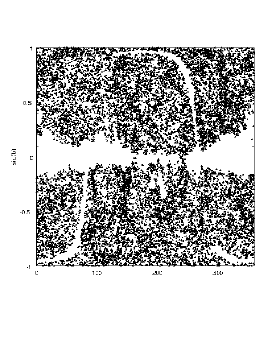
Figure 2: Sky distribution of PSCz galaxies

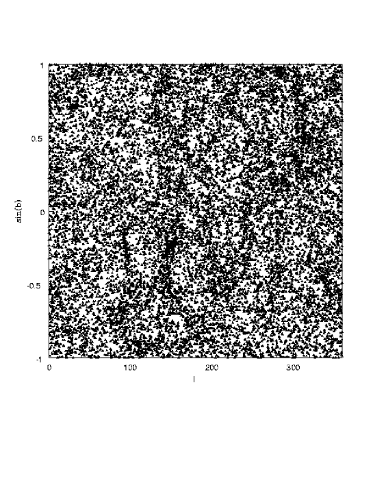
Figure 3: Sky distribution of PSCz galaxies, with mask filled by sampling average sky

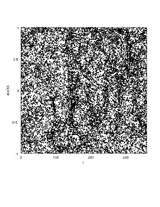
Figure 4: Sky distribution of PSCz galaxies, with mask filled by sampling neighbouring bins

Figure 5: Sky distribution of PSCz galaxies without measured redshift.

4 Dipole in local and CMB frames

Figure 6: Observed dipole amplitude in Local Group (x’s) and CMB (filled triangles) frames, and with crude flow model (see text - filled circles).

In linear theory the peculiar velocity at position $\bf{r}$ can be derived as (Peebles 1980)

$\bf{V(r)}$ = $(H_{o}\beta/4\pi)\int\delta(\bf{r^{\prime}})(\bf{r}-\bf{r^{\prime}})/|\bf{r}-\bf{r^{\prime}}|^{3}$ $d^{3}r^{\prime}$ , (1)

where $\delta=\delta\rho/\rho$.

For a redshift survey of a galaxy population which samples the density field and satisfies a universal luminosity function $\eta$(L,z), independently of $\delta(\bf{r^{\prime}})$, the RHS of eqn (1) can be evaluated as

$(H_{o}\beta/4\pi n)\Sigma(\bf{r}-\bf{r^{\prime}})/(\phi(|\bf{r}-\bf{r^{\prime}}|)|\bf{r}-\bf{r^{\prime}}|^{3})$ , (2)

where n is the average density of galaxies and $\phi(r)$ is the selection function. We refer to $\bf{V(0)}$, the predicted velocity of the Local Group, as the cosmological dipole. The problem is that eqn (2) requires us to know the true distance of galaxies, whereas we know only the observed radial velocity, which includes the effect of the galaxy’s peculiar velocity.

We have first calculated the dipole as in Rowan-Robinson et al (1990) for several different assumptions about the velocity field.

(1) In the Local Group frame, correcting only for the effects of Galactic rotation. This would be valid if the CMB dipole was generated at distances beyond those sampled by the PSCz data.

(2) In the CMB frame. This would be valid if the CMB dipole were generated very locally.

(3) In a crude model for the velocity field, in which no correction (apart from Galactic rotation) is applied to galaxies with recession velocity V $<V_{o}$, whereas galaxies with V $>V_{o}$ are corrected for the CMB motion. This assumes that galaxies with V $<V_{o}$ move together as a block. $V_{o}$ was taken as 3000 km/s.

Figs 6 show the dipole amplitude, summed out to distance d, as a function of d, in these 3 models for the augmented data with the masked area filled according to prescription (D) (spherical harmonics).

Clearly different flow models can dramatically affect the dipole amplitude.

We use model (3) as the starting point for our iterative derivation of the dipole in real space in section 6.

5 Cluster and void model for observed density distribution

In order to correct the observed redshifts for peculiar motions and convert to real space, we follow an approach similar in spirit to that of Rowan-Robinson et al (1990). We seek to make an analytic model of the density field, from which the implied peculiar velocities can be calculated and corrected.

The quality of the PSCz data allows us to be far more ambitious with this model than Rowan-Robinson et al (1990), whose model used only 10 clusters (and no voids). Here we try to use all prior knowledge about galaxy clustering out to 30,000 km$/$s. Our initial input cluster lists consists of

• (1) the galaxy groups with V $<$ 2500 km/s from Rowan-Robinson (1988), which are in turn based on group lists by de Vaucouleurs (1976) and Geller and Huchra (1983). These are included to try to give some resolution of nearby structure.

• (2) a compilation of Abell clusters with V $<$ 30000 km/s (Abell et al 1989, Postman et al 1992, Dalton et al 1994).

• (3) an additional list of clusters for which distance estimates have been given in the literature (Sandage 1975, Lucey and Carter 1988, Mould et al 1991, 1993).

Because of the good all-sky sampling of the PSCz survey it is worthwhile to supplement these lists with clusters and voids found in the PSCz data set itself as follows. The data binned in 100 sq deg bins as in section 3 is further binned in 40 velocity bins, whose boundaries are chosen using the selection function to give the same number of galaxies in each velocity bin (on average about 1 per bin). The 413 x 40 array is then searched for bins in which the number of galaxies exceeds a threshold (taken to be 4 galaxies in a bin) to yield a supplementary list of clusters. The array is also searched for voids, which are defined to be sequences of 5 contiguous velocity bins containing no galaxies. A few (25) additional potential clusters which seemed to be visible in the 3-dimensional distribution, but which were missed by this procees, were inserted by hand (numbered PC1000 onwards).

The complete list of clusters and voids is subject to a neighbours search to weed out duplicates.

(a) d $<$ 25 $h^{-1}$ Mpc

• rationalize all cluster or group pairs within 2 $h^{-1}$ Mpc of each other (this eliminates 6 nearby groups)

• eliminate all PSCz-selected clusters within 4 $h^{-1}$ Mpc of known groups or clusters

• rationalize void pairs within 4 $h^{-1}$ Mpc of each other

(b) d $>$ 25 $h^{-1}$ Mpc

• rationalize all cluster pairs within 4 $h^{-1}$ Mpc of each other (this eliminates 21 clusters)

• eliminate all PSCz-selected clusters within 8 $h^{-1}$ Mpc of a known cluster

• rationalize void pairs within 8 $h^{-1}$ Mpc of each other

This procedure is necessary to avoid clusters disrupting their neighbours during the iteration. The final input cluster list contains 88 nearby groups, 854 clusters and 163 voids (cluster/void list and parameters for final flow model available by ftp). An iterative least-squares process now selects the PSCz galaxies within a specified distance of the cluster or void centres and looks for infall (clusters)

$V=Ar^{-\alpha}$, (3)

(equivalent to a characterist density profile $\rho(r)\propto r^{-1-\alpha}$)

or outflows (voids)

$V=Ar$.

(valid for a region of constant below-average density)

If a void is found to be completely empty of galaxies, so A can not be estimated in this way, then A is set to be

A = 100 $h\beta/3$

which is the relevant value for an empty void.

From a least-squares analysis we find $\alpha=0.6\pm 0.1$ for cluster infall and we adopt the value $\alpha$ = 0.6.

We set a limit for the size of clusters and voids defined as follows:

• for nearby groups (and voids) within 25 $h^{-1}$Mpc, a maximum radius of 4 $h^{-1}$Mpc, except for the Virgo, Fornax and Puppis clusters, and the Local Void (see below):

• for all other clusters within 100 $h^{-1}$Mpc, a maximum radius of 16 $h^{-1}$Mpc:

• for all other voids within 100 $h^{-1}$Mpc, a maximum radius of 8 $h^{-1}$Mpc:

• for clusters with distances greater than 100 $h^{-1}$Mpc, a maximum radius of 32 $h^{-1}$Mpc:

• for voids with distances greater than 100 $h^{-1}$Mpc, a maximum radius of 16 $h^{-1}$Mpc.

A maximum size has to be set to prevent clusters swallowing their neighbours. The increase in maximum size with distance reflects the worsening resolution of the model.

The cluster-void model is then used to predict the peculiar velocity field and the radial distance of each PSCz galaxy is adjusted accordingly before entering the next iteration. The triple-valued zone around each cluster is treated as follows. For a cluster with amplitude A, a core radius $(A/100)^{1/(1+\alpha)}h^{-1}$Mpc is defined within which infall to the cluster can overwhelm the Hubble flow. Within this zone there is ambiguity about which side of the cluster the galaxy lies on (in front or behind). If the cluster model places the galaxy within this distance of the centre of the cluster, the galaxy is assigned a distance equal to that of the cluster centre and then is not included in the infall solution. To avoid excessive feedback, the core radius is in practice damped by multiplying by 0.75. Without this, clusters tend to grow in size and swallow all the galaxies around them into their core, thereby disappearing from the solution.

The local volume, d $<$ 25 h^-1 Mpc, requires especial care, as the resolution of the IRAS sample is not adaquate for arriving at an accurate model. It is clear that Virgo and Eridanus-Fornax are dominant structures in the local flow. There is the possibility of additional significant structures behind the Galactic plane. For example it has been proposed that there is an important local structure in the direction of Puppis (Lahav et al 1993) and several other groups or clusters within this volume at $|b|<20^{o}$ have been identifed in the PSCz cluster searches described above. Finally, inspection of the 3-dimensional galaxy distribution shows that the Local Void (Saunders et al 1991) occupies most of one quadrant of the local volume. These structures have been treated as follows: Virgo, Eridanus, Puppis and the other clusters/groups at $|b|<20^{o}$ were allowed to grow to a maximum size of 16 $h^{-1}$Mpc, ie they were assumed to be comparable to an Abell cluster. The Local Void was allowed to grow to a maximum size of 8 $h^{-1}$Mpc, ie was assumed to be comparable to other voids at d $<$ 100 $h^{-1}$Mpc . The resulting model of the local flow can be compared with the results form the Least Action analysis of Sharpe et al (1999), in which the orbits of the nearby galaxies are followed in detail. To bring our results into agreement with those of Sharpe et al, we had to move the centre of the Local Void from d = 25 $h^{-1}$Mpc, estimated by Saunders et al (1991) from analaysis of the QDOT sample, to 9 $h^{-1}$Mpc. At this distance it exerts a dynamic effect on our Galaxy comparable to that of the Virgo cluster. The Puppis cluster was not found to have a very strong effect on our Galaxy’s motion. However two other clusters, PC1000 at (l,b) = (310,5), d = 14.5 $h^{-1}$, and PC1001 at (l,b) = (279,10), d = 28.4 $h^{-1}$Mpc, proved to be important new structures, with mass comparable to Virgo (the centre of the former lies in the masked region, and it is less prominent when the mask is filled homogeneously). In order of the peculiar velocity generated at the Local Group (given in brackets in km s^-1), the 10 most significant individual structures are Virgo (162), the Local Void (127), PC1000 (119), PC1001 (67), AWM7 (part of Per-Pis, 62), A3526 (Cen, 42), A2052 (Her, 40), N2997 gp (33), A3565 (N.Cen, 31), and S805 (Pavo, 29).

The goodness of fit of the infall model for clusters can be tested by calculating the change in $\chi^{2}$ when the model is implemented, using the velocity error estimates of Tayor and Valentine (1999). For the spherical harmonic mask-fill, $\chi^{2}$ changes from 8247 to 4583 for 4111 degrees of freedom, demonstrating that the fit to the local infall by eqn (3) is good.

6 Dipole in real space

The cluster-void model is used, as described in the previous section, to convert the PSCz data to a real space data set. Note that this model is fully non-linear, to within the limitations implied by the assumed spherical symmetry of the clusters and voids, although the data to which it is being fitted are based on the linear assumption (eqn (1)). The initial velocity field is defined by the crude model (3) of section 3, and is then improved in a series of iterations until a a self-consistent model of the flow-field is obtained. We have also iterated the value of $\beta$ in eqn (1) in order to arrive at a fully self-consistent flow model.

Figure 7: Observed dipole components in real space, mask filled by spherical harmonics. Solid line shows prediction of cluster+void model.

Figure 8: Observed dipole components in real space, mask filled by average sky. Solid line shows prediction of cluster+void model.

Figure 9: Observed dipole amplitude in real space, mask filled by spherical harmonic model (filled circles). Solid line shows prediction of cluster+void model.

Figure 10: Observed dipole amplitude in real space, mask filled by average sky (filled circles). Solid line shows prediction of cluster+void model. Results from QDOT analysis (Lawrence et al 1999) shown as filled triangles.

Fig 7,8 shows the components of the dipole in real space, with the predictions of the cluster-void model, for the two different mask treatments (C) and (D). The fit of the cluster/void model to the PSCz dipole components is excellent. In calculating the dipole from IRAS galaxies we have excluded the contribution of galaxies within 4 $h^{-1}$ Mpc. Similarly in computing the total dipole contribution of the cluster and group model we have excluded groups within the same volume. The lack of adaquate sampling in the local volume could result in a constant offset vectors between each of the IRAS dipole, the cluster+void model dipole, and the true dipole. The CMB dipole also has to include the not very well determined vector of the sun’s motion with respect to the Local Group of galaxies. We have assumed that the sun’s velocity with respect to the Local Group is 300 km$/$s towards (l,b) = (90,0), consistent with the values measured by Yahil et al (1977). The offset found between the PSCz dipole and the CMB direction is 21.7^o at 150 $h^{-1}$Mpc, 18.0^o at 200 $h^{-1}$Mpc, 15.5^o at 250 $h^{-1}$Mpc, and 13.4^o at 300 $h^{-1}$Mpc. Strauss et al (1992) analyzed the expected offset in a range of models using simulations and compared these predictions with the data for the 1.2 Jy sample. Although the misalignment between the IRAS and CMB dipoles has been advocated as a test of cosmological parameters (Juskiewicz et al 1990, Lahav et al 1990, Strauss et al 1992), the problem is that density structure in the masked region could have a strong effect on the x and y components (especially the x component). It is noticable that the component which shows the greatest discrepancy with the CMB dipole is the x-component. A cluster behind the Galactic centre at the distance of, and with twice the mass of, the Centaurus cluster (A3526) would bring the dipoles to alignment within 5^o. Since such a hypothetical object can not be rules out, there is little cosmological information in the dipole misalignment. Other possible reasons for misalignment are that IRAS galaxies may be subtly biased with respect to the mass distribution or that there may be non-linear corrections to eqn (1).

Fig 9,10 shows the total dipole amplitude as a function of distance for the two assumptions about the mask. The uncertainties in the dipole amplitude for the PSCz sample have been estimated by Taylor and Valentine (1999), including the effects both of cosmic variance and shot noise and these are included in Figs 9, 10. The prediction for the cluster/void model is also shown in each case. There is some difference between the predicted dipole amplitudes for the two mask-filling assumptions, amounting to 140 $km/sec$ at 200 $h^{-1}$ Mpc for an assumed $\beta$ =1. Thus some of the disagreements about values of $\beta$ in different studies stem from different assumptions about how to fill the mask. It is clearly worth investigating other methods of filling the masked sky. However the missing information can not actually be recovered and we have to regard the different amplitudes found from the two methods of filling the mask as indicative of the uncertainty induced by the incomplete sky coverage of PSCz. Also plotted in Fig 10 is the dipole amplitude from the QDOT study by Rowan-Robinson et al (1990, as corrected by Lawrence et al 1999), which should be comparable with the case where the mask is filled by the average sky. The agreement is excellent over the distance range in common.

Other approaches to the problem of dynamical reconstructing include the iterative schemes of Yahil et al (1991) and the spherical harmonic analysis with Wiener filtering of Fisher et al (1995), Heavens and Taylor (1995). Our method is not only stabler than the method of Yahil et al (1991), but it also yields an analytic model of the flow throughout the survey volume. The spherical harmonic approach is less subject to the bias of starting from known cluster and group lists, entailed in our approach. However there is a considerable cosmographic benefit in being able to relate the flow to identifiable structures and in a subsequent paper we will demonstrate the benefit of this for studies of the Hubble constant (and claimed anomalies like the Lauer-Postman effect).

Since we can be sure that some galaxy structures extend across the masked regions, the treatment of filling the mask homogeneously is unlikely to be realistic, so in what follows we give results for the case where the mask is filled using spherical harmonics.

Table 1: PSCz and cluster/void model dipoles as a function of depth, mask filled by average sky

	PSCz						cluster
							model
d($h^{-1}$ Mpc)	$V_{x}$	$V_{y}$	$V_{z}$	$V_{tot}$	l	b	$V_{x}$	$V_{y}$	$V_{z}$	$V_{tot}$	l	b
10.	-68.8	-114.7	43.3	140.6	239.1	18.0	-6.2	-31.6	34.4	47.1	258.9	46.9
20.	-81.7	-220.1	150.4	278.9	249.6	32.6	-39.8	-265.8	241.2	361.2	261.5	41.9
30.	-62.6	-360.4	246.3	440.9	260.1	34.0	-0.4	-392.7	278.5	481.8	269.9	35.3
40.	-66.3	-420.6	262.7	500.3	261.0	31.7	-9.5	-470.7	329.9	575.3	268.8	35.0
50.	-105.3	-429.4	241.0	503.5	256.2	28.6	-73.4	-478.8	267.1	553.6	261.3	28.8
60.	-111.3	-431.0	175.0	478.3	255.5	21.5	-92.0	-465.2	226.9	526.3	258.8	25.5
70.	-131.9	-434.5	194.5	494.0	253.1	23.2	-122.8	-442.6	240.3	518.9	254.5	27.6
80.	-126.9	-430.4	264.4	520.8	253.6	30.5	-120.8	-439.3	285.5	538.1	254.6	32.0
90.	-159.0	-463.2	261.3	555.1	251.1	28.1	-127.8	-418.8	287.4	524.3	253.1	33.2
100.	-149.1	-442.8	299.2	554.8	251.4	32.6	-147.1	-428.7	271.8	529.0	251.1	30.9
110.	-133.9	-438.6	322.0	560.3	253.0	35.1	-138.4	-413.9	325.8	545.1	251.5	36.7
120.	-135.6	-428.9	328.7	557.1	252.5	36.2	-179.2	-433.7	307.1	561.3	247.6	33.2
130.	-168.4	-445.3	363.4	598.9	249.3	37.4	-161.5	-465.8	307.8	581.7	250.9	31.9
140.	-186.6	-435.6	391.0	614.3	246.8	39.5	-173.6	-464.7	308.3	584.5	249.5	31.8
150.	-197.2	-443.2	383.8	618.6	246.0	38.4	-162.9	-491.5	331.8	615.5	251.7	32.6
160.	-200.7	-448.6	405.1	636.8	245.9	39.5	-155.0	-481.9	310.7	594.5	252.2	31.5
170.	-189.3	-464.5	370.7	623.7	247.8	36.5	-165.8	-492.8	334.5	618.7	251.4	32.7
180.	-161.9	-489.3	352.4	624.3	251.7	34.4	-172.8	-509.4	333.8	633.5	251.3	31.8
190.	-152.5	-471.7	354.4	609.4	252.1	35.6	-156.0	-506.8	325.6	622.8	252.9	31.5
200.	-188.9	-494.0	360.9	640.3	249.1	34.3	-168.2	-507.1	309.8	618.1	251.7	30.1
210.	-168.1	-536.8	342.1	658.4	252.6	31.3	-164.9	-504.9	311.2	616.1	251.9	30.3
220.	-200.2	-552.1	348.5	682.9	250.1	30.7	-169.8	-513.2	319.9	628.6	251.7	30.6
230.	-193.3	-552.4	338.1	675.9	250.7	30.0	-161.9	-529.6	303.4	632.0	253.0	28.7
240.	-175.3	-556.5	310.9	661.1	252.5	28.0	-165.1	-533.1	313.9	640.8	252.8	29.3
250.	-203.4	-578.4	312.0	687.9	250.6	27.0	-167.0	-527.9	304.6	632.4	252.5	28.8
260.	-160.1	-567.9	320.4	671.4	254.3	28.5	-168.6	-526.5	309.1	633.9	252.3	29.2
270.	-162.3	-594.9	330.0	699.3	254.7	28.2	-170.0	-527.3	308.1	634.5	252.2	29.1
280.	-167.7	-643.0	391.7	771.4	255.4	30.5	-171.0	-526.8	302.0	631.3	252.0	28.6
290.	-173.7	-565.5	344.4	684.5	252.9	30.2	-171.0	-526.8	302.0	631.3	252.0	28.6
300.	-179.1	-584.3	302.1	681.7	253.0	26.3	-171.0	-526.8	302.0	631.3	252.0	28.6
					CMB		-25.2	-545.4	276.5	612 $\pm$ 22	268 $\pm$ 3	27 $\pm$ 3

7 Convergence of the dipole and the value of $\beta$

Previous studies of the IRAS dipole have been limited to d $\leq$ 150 $h^{-1}$Mpc. Our larger sample allows us to investigate the convergence of the dipole to a significantly greater depth. Although there are massive structures in the distance range 150-300 $h^{-1}$Mpc, it appears that the impact of these structures on the motion of the Local Group is small. The change in dipole amplitude from 150 to 300 $h^{-1}$Mpc is no greater than 70 km$/$s. The Shapley cluster concentration, for example, proposed by Raychaudhury (1989), Scaramella et al (1989), and Plionis and Valdarnini (1991) as a major contributor to the Local Group’s motion, contributes only 21 km$/$s. The results found here for d $>$ 150 $h^{-1}$Mpc appear to differ from those of Strauss et al (1992) based on the 1.2 Jy sample, who saw a steep increase in dipole amplitude between 150 and 200 $h^{-1}$Mpc. However this can probably be attributed to the increased shot noise associated with the smaller sample.

Vittorio and Juskiewicz (1987) raised the question of whether the calculation of eqn (1) can in fact be a convergent process and this has been discussed in many subsequent papers (eg Juskiewicz et al (1990), Lahav et al (1990), Peacock (1992) and Strauss et al (1992)). The growth of the dipole amplitude at large distances clearly depends on the spectrum of density perturbations on large scales. The fact that we empirically find convergence (in the sense that the dipole amplitude changes by no more than 10$\%$) over a range of distances corresponding to an increase in volume of a factor of 8 is itself a significant constraint on the large scale spectrum. Peacock (1992) emphasizes that plateaus of apparent convergence can appear in simulations even when the the dipole amplitude is far from the asymptotic value. However the fact that we are seeing convergence over scales approaching those on which the microwave background radiation is known to be extremely smooth does not leave much scope for significant jumps in the dipole amplitude at larger distances than those surveyed here.

The IRAS selection at 60 $\mu$m undersamples the elliptical galaxy population, and hence the dense cores of rich clusters. However these cores represent only a few percent of the total masses of the clusters characterized here, which tend to be of supercluster dimensions. Strauss et al (1992) have shown that correction for this undersampling of cluster cores changes the dipole amplitude by at most a few percent.

Table 1 gives the dipole components, total amplitude and direction as a function of distance, together with the corresponding quantities for the cluster/void model. The amplitudes and directions can be compared with the results of COBE (Kogut et al 1993, Fixsen et al 1996), which can be combined with the estimate of the velocity of the sun relative to the Local Group to give the values shown in the last line of the Table. From the values at 200 $h^{-1}$Mpc, beyond which we find no evidence for a significant contribution to the dipole, we conclude that $\beta$ = 0.75, with a $1-\sigma$ range of 0.67-0.86 and a $2-\sigma$ range of 0.60-1.01. The uncertainty in $\beta$, derived from the analysis of Taylor and Valentine (1999), includes the effects of shot noise and cosmic variance, but does not include the uncertainties associated with the mask-filling assumptions. From repeated realizations of the average sky mask-filling, we estimate the statistical contribution to the uncertainty in $\beta$ to be only $\pm$0.05, for a given assumption about how the mask should be filled. However changing from the spherical harmonic mask-fill to an average sky mask-fill resulted in a shift of $\beta$ by 20$\%$, which can be taken as an indication of the maximum additional systematic uncertainty associated with the mask. For b = 1, the corresponding value of $\Omega_{o}$ = 0.62, with a $1-\sigma$ range of 0.51-0.78 and a with a $2-\sigma$ range of 0.43-1.02. Values of $\Omega_{o}$ outside this range would probably require pathological behaviour of the density fluctuation spectrum. The present work can not decisively choose between current popular models with $\Omega_{o}=1,\Lambda=0$ and $\Omega_{o}=0.3,\Lambda=0.7$, though the former is slightly preferred.

Our value of $\beta$ can be compared with those derived from other studies of the PSCz sample: 0.7 +0.35, -0.2 from a likelihood analysis of the Local Group acceleration (Schmoldt et al 1999), 0.58 $\pm$ 0.26 from spherical harmonic analysis of the redshift space distortion (Tadros et al 1999), 0.6 +0.22, -0.15 from a study of the cosmic velocity field (Branchini et al 1999). Our result is clearly consistent with all of these, which is impressive given the very different approach to modelling the density field used in these different studies. Our results are also consistent with the earlier results using previous IRAS samples summarized by Rowan-Robinson (1997, summary value 0.85 $\pm$ 0.15), and with subsequent results from da Costa et al (1998) and Sigad et al (1998) (0.6 $\pm$ 0.1 and 0.89 $\pm$ 0.12, respectively).

8 Cluster masses

The mass of each cluster (or mass-deficit of each void) can be calculated from

$M_{cl}=(4\pi/3)\int\rho^{\prime}r^{\prime 2}dr^{\prime}$

= 3 $(\Omega_{o}/\beta)H_{o}(Ar_{cl}^{1.4})/2G$

= 3.6 x 10${}^{10}Ar_{cl}^{1.4}hM_{\odot}$ . (3)

The results are given in Tables 2-12 for each cluster detected with $A/\sigma_{A}>$ 1.0. Fig 11 shows the distribution of cluster masses with distance. The loss of resolution with increasing distance means that only very large structures can be detected at large distances. The masses in the Hydra-Centaurus, Pavo-Indus, Perseus-Pisces-Cetus, Coma-A1367, Hercules and Shapley supercluster complexes are respectively 7.1, 4.4, 11.8, 6.5, 34.2, 16.5 x 10${}^{15}M_{\odot}$ compared to the Virgo cluster mass of 1.3x10${}^{15}M_{\odot}$. Our cluster masses our generally substantially larger than the estimates given for the region within an Abell radius, since they include the extensive halo of galaxies extending out to tens of Mpc around each cluster.

Figure 12 gives a histogram of the number of clusters and groups in the input list (dotted histogram), together with those detected in the PSCz sample (solid, shaded histogram). Out to d = 150 $h^{-1}$ Mpc, about 60 $\%$ of clusters are detected, but beyond this distance there is a steady fall in the percentage of clusters detected, reflecting the selection function of Fig 1.

Figure 13 shows the average density fluctuation

$\delta\rho/\rho=3M/4\pi\rho_{o}r_{cl}^{3}$

as a function of cluster radius $r_{cl}$. If we take the median value as indicative of $<\delta\rho/\rho(r_{cl})$, then we find

$<\delta\rho/\rho>\propto r^{-0.75}$, for 2 $\leq$ d $\leq$ 32 $h^{-1}$ Mpc,

comparable with the findings of Sutherland et al (1999).

Figure 11: Masses of clusters and voids (in units of $10^{14}M_{\odot}$) as a function of distance.

Figure 12: Histogram of clusters in input catalogue (broken curve) and those detected as structures in PSCz (shaded).

Figure 13: The average value of $\delta\rho/\rho$ in a cluster versus cluster radii. The solid line corresponds to $\delta\rho/\rho\propto r^{-0.75}$, corresponding to $P(k)\propto k^{-1.5}$, in agreement with the power spectrum derived by Sutherland et al (1999).

9 The flow field predicted by IRAS

Fig 14 shows the distribution in Supergalactic coordinates (z-axis towards (l,b) = (47, 6), x-axis towards (l,b) = (137, 0)) of galaxies within 22.5^o of the Supergalactic plane, with the direction of their predicted flow (eqn 1) indicated. The strong concentrations towards Virgo, Hydra-Centaurus and Perseus-Pisces are clearly seen. Fig 15 shows the corresponding distribution for cluster centres, with the velocities predicted by the cluster-void model. A detailed discussion of the flow field derived from PSCz is given by Saunders et al (1999).

In a later paper we will use the peculiar velocities of the clusters to study the Hubble diagram for those clusters for which a distance is known and will give an analysis if the Lauer and Postman result.

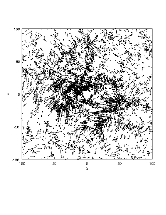
Figure 14: Galaxies within 22.5^o of the Supergalactic plane, with the direction of their predicted motion, in the CMB frame, indicated.

Figure 15: Clusters within 22.5^o of the Supergalactic plane, with the direction of their predicted motion indicated.

10 Summary

(1) We have investigated the convergence of the cosmological dipole using the new PSCz IRAS galaxy redshift survey.

(2) The amplitude of the calculated dipole depends on the assumption used to fill the masked area of the sky and this accounts for some of the differences between previous results.

(3) The PSCz identifications appear to be substantially complete to d = 300 $h^{-1}$ Mpc for areas of the sky with I(100) $>$ 12.5 MJy$/$sr. Between I(10) = 12.5 and 25 MJy$/$sr, the completeness limit declines to 150 $h^{-1}$ Mpc. This effect was corrected by adding additional sources in this zone based on a spherical harmonic analysis of the unmasked sky.

(4) The dipole appears to have converged by 200 $h^{-1}$ Mpc. Between 200 and 300 $h^{-1}$ Mpc, the additional contribution to the dipole amplitude is estimated to be $\leq$ 40 km$/$s. Rather special and pathological assumptions about the power spectrum of density fluctuations would be required to achieve consistency with the present data and the CMB fluctuations, yet result in a very different asymptotic dipole amplitude.

(5) The direction of the dipole calculated from IRAS galaxies (the direction in which the Local Group is being pulled) is 13^o away from the CMB dipole (the direction in which the Local Group is moving), the main uncertainty in direction being associated with the masked area behind the Galactic plane. The improbability that further major contributions to the dipole amplitude will come from volumes larger than those surveyed here means that the question of the origin of the CMB dipole is essentially resolved.

(6) The correction of the observed (heliocentric) velocities to real space distances is performed using an analytic model of the flow field involving 842 clusters and 163 voids, with all Abell clusters within 300 $h^{-1}$ Mpc involved in the solution. About 60 $\%$ of clusters with d $<$ 150 $h^{-1}$ Mpc are detected as significant dynamical objects. Inferred masses for Abell clusters are in the range 1 - 300 x 10${}^{14}M_{o}$. The Local Void and two new nearby (d $<$ 30 Mpc) clusters identified close to the Galactic plane at (l,b) = (310,5), (279,10) have a major effect on the Local Group motion. It will be interesting to see if redshift surveys within the masked area of the Galactic plane can confirm the scale of these structures.

(7) When the mask is filled with a Poissonian distribution of sources typical of the average unmasked sky, a value for $\beta$ = 0.90 $\pm$ 0.15 is found, in excellent agreement with the results found from QDOT (Rowan-Robinson et al 1990, Lawrence et al 1999). For a spherical harmonic mask-fill, which is probably the most realistic assumption to make about how the mask should be filled, we find the value of $\beta$ = 0.75 +0.11,-0.08. For b =1 this corresponds to $\Omega_{o}$ = 0.62, with a 2-$\sigma$ range of 0.43-1.02. Alternatively $\Omega_{o}$ = 1 requires a bias factor b = 1.33 $\pm$ 0.17. The maximum additional systematic uncertainty associated with our ignorance of the masked region is estimated to be $\pm$20$\%$.

Table 2: Groups and clusters with $V_{obs}<2500km/s$

name	l	b	$V_{obs}$	$V_{CMB}$	A	$r_{cl}$	$S/N$	$V_{LG}$	$M_{cl}(10^{12})M_{\odot}$	other name
R1 N134	21.8	-86.1	1609.0	1462.6	492.4	3.	4.7	11.6	89.3
R3 N448	136.6	-63.9	1748.0	1309.4	305.7	4.	2.6	12.4	76.6
R6 CETII	152.6	-67.7	1827.0	1653.0	203.5	4.	4.9	5.2	51.0
R8 CETI	169.0	-55.3	1433.0	1050.2	134.5	2.	3.7	3.2	12.8	R10
R11 N1248	180.1	-46.5	2088.0	1943.1	306.8	4.	3.1	5.7	76.9
R12 ERIDAN	207.3	-51.8	1549.0	1619.9	441.9	5.	6.8	16.2	153.1
R13 FORNAX	236.4	-54.3	1311.0	1535.9	367.4	4.	2.3	10.8	92.1
R17 N1800	234.4	-35.1	841.0	1035.4	277.6	4.	3.1	18.0	69.6
R21 N2577	201.1	29.6	2000.0	2604.1	99.6	4.	1.3	1.0	25.0
R25 N2964	194.6	49.0	1537.0	2046.9	365.8	3.	7.0	4.4	66.4
R28 N2997	263.9	20.0	684.0	905.0	389.6	4.	4.1	33.1	97.7
R29 N3166	238.2	45.5	1118.0	1723.7	180.6	4.	2.3	4.2	45.3
R31 N3190	213.0	54.9	1246.0	1786.4	142.0	3.	4.3	2.2	25.8
R33 LEO	232.6	61.3	1012.0	1452.0	275.8	4.	6.8	9.1	69.1
R35 N3504	204.6	66.0	1392.0	1936.9	212.7	4.	6.4	3.9	53.3
R39 UMAI(N	144.5	58.7	1320.0	1549.4	210.1	3.	2.7	4.4	38.1
R41 N4027	286.1	41.6	1439.0	1813.2	415.3	4.	11.7	8.8	104.1
R44 N4120	129.3	49.2	2407.0	2547.2	146.6	4.	1.1	1.6	36.8
R45 COMAI	192.0	82.6	827.0	793.7	210.2	4.	6.5	23.2	52.7
R47 VIRGO	283.8	74.5	1016.0	1312.7	760.4	16.	12.3	162.2	1327.7
R49 N4729	302.6	21.6	1893.0	2113.8	380.0	4.	2.5	5.9	95.3
R51 N5033	99.2	79.9	981.0	1282.4	285.8	3.	5.7	8.8	51.9
R52 N5061	310.3	35.7	1803.0	2019.7	347.6	2.	5.5	2.2	33.0
R56 N5336	89.5	69.7	2352.0	2534.9	196.4	3.	1.8	1.1	25.8
R58 N5422	103.5	59.3	2057.0	2273.9	77.4	4.	1.1	1.0	19.4
R59 N5483	317.8	17.3	1277.0	1575.3	402.8	3.	9.9	5.9	52.9
R62 VIRGOI	354.4	56.7	1614.0	2125.7	236.5	2.	3.0	1.4	22.5
R70 GRUS	348.1	-65.2	1614.0	1606.2	88.3	2.	1.0	0.9	8.4
PUPPIS	240.0	0.0	1500.0	2032.8	614.8	5.	13.0	14.3	213.0

Table 3: PSCz groups with $V_{obs}<2500km/s$

name	l	b	$V_{obs}$	$V_{CMB}$	A	$r_{cl}$	$S/N$	$V_{LG}$	$M_{cl}(10^{12})M_{\odot}$	other name
PC190	210.0	-16.0	1906.9	2295.6	405.0	5.	4.6	7.4	140.3
PC222	245.0	0.0	2218.1	3075.0	495.9	10.	3.4	13.3	453.4
PC291	248.8	20.0	1807.2	2535.2	375.5	4.	3.5	4.1	94.1
PC315	249.7	30.0	2246.3	3066.3	273.5	3.	3.7	1.5	49.6
PC322	307.7	30.0	2284.4	2637.4	594.5	3.	13.3	3.1	78.1
PC328	319.4	30.0	2320.9	2697.3	202.2	3.	13.8	1.0	26.5
PC364	353.6	40.0	2044.4	2588.7	264.8	4.	6.6	2.8	66.4
PC388	305.2	50.0	1422.4	1901.0	162.0	3.	8.6	1.6	21.3
PC415	290.0	60.0	2349.0	2959.7	110.6	3.	3.2	0.6	20.1
PC436	285.0	70.0	2280.0	2836.5	151.1	3.	7.7	0.9	27.4
PC1000	310.0	5.0	1255.2	1451.3	592.8	16.	5.9	119.1	1035.1
PC1001	279.0	10.0	2207.2	2839.5	1112.1	16.	14.7	66.9	1941.8

Table 4: Abell and other clusters with $V_{obs}=2500-15000km/s$

name	l	b	$V_{obs}$	$V_{CMB}$	A	$r_{cl}$	$S/N$	$V_{LG}$	$M_{cl}(10^{12})M_{\odot}$	other name
A2731	313.9	-59.3	9354.0	9531.8	817.7	10.	2.8	2.3	747.7
N80	114.0	-40.0	6268.0	5912.4	541.4	8.	5.5	2.8	358.2	GH3
N128	112.0	-60.0	4657.0	3703.8	329.0	16.	2.4	11.6	574.5	GH6
N194	117.0	-60.0	5298.0	4789.5	1600.2	6.	8.4	9.3	766.2
A76	117.8	-56.0	11990.0	11580.9	1098.6	25.	1.8	7.6	3663.3
S109	284.7	-86.0	9473.0	9494.2	1154.6	16.	4.4	6.2	2016.1
PISC	127.0	-30.0	5306.0	5143.8	445.6	16.	1.9	8.2	778.1	GH8,GH9,N383,3C3
A2870	294.8	-70.0	6593.0	6473.4	272.2	8.	13.0	1.2	180.1
A2877	293.1	-70.9	7105.0	7207.9	416.6	16.	2.4	3.9	727.4
A2881	148.5	-79.0	13311.0	12970.4	893.8	32.	2.2	6.8	4118.6
A189	139.3	-60.2	9840.0	9505.9	1275.6	8.	9.5	2.6	844.0
A193	136.9	-53.3	14453.0	14501.4	617.0	20.	1.8	2.0	1488.8
A194	142.1	-63.1	5479.0	5142.4	1222.6	16.	9.4	22.4	2134.8	GH15,N547,3C40
0131-36	261.0	-77.0	8940.0	8995.2	420.3	8.	18.5	1.0	278.1
A260	137.2	-28.0	11062.0	11282.7	647.9	32.	1.2	6.5	2985.5
A262	136.6	-25.1	5094.0	4087.9	1735.0	10.	9.8	26.4	1586.4
N741	151.0	-54.0	5637.0	5410.8	436.0	13.	1.4	5.2	550.9	GH23
S250	273.4	-60.5	14510.0	14667.8	999.1	25.	2.3	4.3	3331.5
A347	141.2	-17.6	5875.0	6313.8	2232.2	16.	7.6	27.2	3897.7
S274	280.2	-54.6	9264.0	9635.9	325.6	16.	1.4	1.7	568.5
N1016	168.5	-51.0	6236.0	6016.1	574.4	16.	2.6	7.7	1003.0	GH30
A376	147.1	-20.6	14843.0	15145.3	1631.7	13.	3.2	2.5	2061.7
A400	170.2	-44.9	7171.0	7148.8	586.1	13.	1.9	4.0	740.6
A426	150.4	-13.4	5510.0	6019.1	409.2	16.	1.3	5.5	714.5	PERSEUS
A3193	262.0	-47.2	10193.0	10381.2	501.1	13.	2.5	1.6	633.2
S463	262.4	-42.3	11812.0	12166.9	1285.6	16.	2.9	4.2	2244.8
N1600	200.0	-33.0	4797.0	4880.1	612.8	16.	6.4	12.5	1070.0
A496	209.6	-36.5	9804.0	9960.2	1126.9	20.	2.1	7.6	2719.2
S487	249.9	-41.5	11152.0	11581.1	1060.3	10.	4.5	2.0	969.5
S497	250.0	-40.5	9863.0	9945.0	436.1	10.	2.0	1.1	398.7
S500	272.7	-38.1	5696.0	6285.8	226.8	4.	1.0	0.4	56.9
A539	195.7	-17.7	8757.0	9385.5	3346.1	13.	4.6	13.3	4227.9
S521	241.1	-34.0	4497.0	4938.5	462.6	16.	2.0	9.2	807.7
S540	246.4	-30.3	10733.0	11116.1	1268.7	25.	2.4	9.5	4230.5
A548	230.3	-24.8	12231.0	12993.8	1346.1	25.	2.3	7.4	4488.6
A3374	226.7	-21.2	14156.0	15179.2	813.0	20.	2.2	2.4	1961.7
A3376	246.5	-26.3	13641.0	14644.0	1200.8	16.	1.5	2.7	2096.7
S584	262.2	-25.6	14180.0	14896.5	1679.1	20.	3.3	5.1	4051.6
A569	168.6	22.8	5871.0	6093.9	559.0	16.	3.8	7.3	976.1
A576	161.4	26.2	11508.0	11845.1	2428.6	32.	4.2	22.2	11191.0
A634	159.4	33.6	7883.0	7970.4	307.1	16.	1.5	2.3	536.2
CANC	203.0	29.0	4790.0	5323.5	455.0	16.	4.8	7.8	794.5	N2563
A779	191.1	44.4	6854.0	7282.8	648.7	16.	4.6	5.9	1132.7	N2832
A957	243.0	42.9	13235.0	14012.3	2098.5	20.	3.3	7.2	5063.6
A999	227.9	52.6	9428.0	10035.4	622.1	20.	1.6	4.1	1501.1	A1016
S636	272.9	19.2	2608.0	3519.1	478.1	16.	3.0	18.7	834.8	ANTLIA,N3528
A1060	269.6	26.5	3449.0	4498.0	1046.4	16.	10.3	25.1	1827.1	HYDRA,N3311
A1139	251.5	52.7	11730.0	12079.8	2670.9	32.	6.2	23.4	12307.5
A1142	240.1	59.2	10827.0	11317.1	813.8	32.	1.1	8.1	3750.0
N3478	166.0	62.0	7645.0	8064.5	1296.2	10.	4.4	5.1	1185.2	GH73
A1177	220.5	66.2	9484.0	10050.1	337.8	13.	1.0	1.2	426.8
N3735	131.8	45.3	2998.0	3193.0	134.6	3.	13.4	0.7	24.4
S665	283.9	24.3	9533.0	10487.0	344.6	32.	1.5	4.0	1587.9
A1267	209.0	71.4	9877.0	10623.1	832.1	32.	3.6	9.4	3834.3
A1308	268.5	53.6	14422.0	15188.4	1349.5	25.	2.0	5.4	4499.9
A1367	234.8	73.0	6344.0	6752.5	1202.7	10.	9.6	6.7	1099.7	GH81,GH90
N4169	197.4	81.1	3957.0	4189.3	185.7	16.	1.9	5.1	324.3	GH101
A3526	302.4	21.6	2792.0	3509.1	1067.4	16.	13.2	42.0	1863.8	CENT,N4696,N4373
A1656	58.1	88.0	6916.0	7494.6	2408.5	16.	12.5	20.8	4205.5	COMA,GH113,N4889
A3537	305.3	30.4	4826.0	5700.7	280.6	16.	2.0	4.2	490.0	N4936
N5044	311.0	46.0	2600.0	3127.7	355.4	10.	7.1	9.2	325.0	GH63,N5077

Table 5: Abell and other clusters with $V_{obs}=2500-15000km/s$ (cont.)

name	l	b	$V_{obs}$	$V_{CMB}$	A	$r_{cl}$	$S/N$	$V_{LG}$	$M_{cl}(10^{12})M_{\odot}$	other name
N5056	67.1	81.7	6865.0	7167.4	965.4	13.	1.8	6.6	1219.8	GH119
A1736	312.6	35.1	13639.0	14755.0	4944.0	25.	1.6	21.0	16485.8	SHAPLEY
A3565	313.5	28.0	3376.0	4114.1	1069.2	16.	12.3	30.6	1866.9	IC4296,N.CEN
S740	314.1	23.6	10073.0	10172.2	720.3	32.	1.9	8.9	3319.1
A3571	316.3	28.6	11518.0	12506.1	3263.3	16.	5.7	10.1	5698.1	A3572
A3575	317.5	28.3	10802.0	10404.5	1514.9	13.	2.9	4.9	1914.1
A3676	0.8	-34.3	12120.0	12270.7	2139.8	25.	2.3	13.2	7135.2
A3677	9.2	-33.4	13830.0	14385.3	2020.5	10.	1.1	2.5	1847.4
N5322	110.3	55.5	2848.0	3143.0	65.4	4.	2.9	0.5	16.4	GH122
Z74-23	350.0	66.0	6025.0	6013.9	310.9	5.	3.0	0.8	107.7	N5416
S754	319.6	26.5	4137.0	5004.4	913.1	6.	9.5	4.8	437.2	N5419,1400-33
A3581	323.1	32.9	6265.0	6698.3	983.2	16.	7.3	10.6	1716.8
N5557	65.3	69.4	3927.0	4070.9	454.2	8.	4.0	5.0	300.5	GH141
A1983	18.9	60.1	13359.0	14370.6	1856.8	25.	2.3	8.3	6191.5
S778	328.7	18.9	7105.0	7538.6	703.8	8.	4.2	2.3	465.7
A2052	9.4	50.1	10614.0	10691.3	3575.2	32.	10.4	40.0	16474.5
A2063	12.8	49.7	10686.0	12046.5	1745.8	25.	2.1	11.1	5821.4
A2147	28.8	44.5	10686.0	10586.7	5539.2	10.	28.0	12.6	5064.7	HERC
A2152	29.9	44.0	11200.0	12700.2	1376.0	32.	2.4	10.9	6340.6	HERC,A2151
A2162	48.4	46.0	9689.0	9794.4	785.9	8.	3.5	1.5	520.0
A3627	325.3	-7.3	4287.0	5038.0	790.9	10.	4.3	7.9	723.2
A2197	64.8	43.8	9220.0	9390.3	2513.0	16.	4.8	13.8	4388.0	A2197
S805	332.3	-23.6	4227.0	4644.9	1275.5	16.	6.3	28.7	2227.2	PAVO II,S129-1
I4797	342.0	-22.0	2653.0	2798.0	527.5	3.	5.3	3.4	95.7
A3656	2.0	-29.4	5777.0	5913.4	1239.5	10.	5.3	9.0	1133.3
S840	341.9	-32.1	4557.0	4804.3	688.3	16.	2.6	14.5	1201.8
PAVO	324.0	-32.0	3785.0	3910.9	796.2	5.	1.6	5.0	275.9	V38,N6876
N6861	355.0	-33.0	2733.0	2703.1	437.6	10.	6.5	15.2	400.1	TEL,V52,GH80
S866	349.5	-34.7	5486.0	5914.2	1176.4	4.	2.9	2.3	294.9
A3698	19.2	-33.3	6018.0	5856.4	476.7	6.	1.1	1.8	228.2
S889	345.3	-37.5	13101.0	12838.7	2506.8	20.	3.2	10.2	6048.8
S894	18.5	-35.3	12261.0	12589.5	687.4	20.	1.0	2.9	1658.7
A3733	17.8	-39.6	11572.0	11467.3	1823.8	25.	3.0	12.8	6081.5
A3742	352.6	-42.2	4813.0	4731.2	887.6	16.	3.5	19.2	1549.8	N7014,INDUS
A3744	21.4	-40.2	9048.0	8702.5	589.9	16.	1.6	3.8	1030.0
A3747	357.5	-42.7	9174.0	8903.0	2094.0	13.	8.4	9.3	2645.9
N7242	91.6	-15.9	6116.0	5902.7	815.7	16.	6.7	11.4	1424.3
S1065	3.2	-62.4	8634.0	8484.0	300.2	16.	1.2	2.0	524.2
N7385	82.0	-41.0	7738.0	7177.9	912.2	10.	2.4	4.5	834.1
A2572	94.2	-38.9	12315.0	11215.6	763.2	16.	1.4	2.9	1332.6
PEGI	88.0	-48.0	4017.0	3383.4	91.9	16.	1.1	3.9	160.5	N7619,GH166
A2589	94.7	-41.2	12696.0	13379.1	1538.0	20.	2.2	5.8	3711.1
A2592	95.5	-40.0	14109.0	14729.6	717.3	20.	1.9	2.2	1730.8
A2593	93.5	-43.2	12509.0	12120.9	4283.7	25.	12.5	27.0	14284.0
A2634	103.5	-33.1	9508.0	9176.6	772.5	8.	5.3	1.7	511.1	3C465
A2657	96.7	-50.3	12182.0	11627.9	1554.2	25.	2.1	10.6	5182.5
A4038	25.1	-75.9	8484.0	8323.3	837.8	10.	1.6	3.1	766.0	KLEM44,2345-28
A2666	106.7	-33.8	8333.0	7913.6	760.6	16.	2.9	5.9	1328.1	GH173
DC0410-62	274.8	-41.9	4873.0	5251.8	784.8	16.	3.0	13.8	1370.3
MKW1	242.2	39.0	6056.0	6689.4	282.0	16.	3.1	3.1	492.4
MKW5	334.7	55.7	7345.0	7695.4	467.1	16.	1.3	3.8	815.6
ZW499-13	113.9	-32.5	7006.0	6719.1	449.3	16.	1.5	4.8	784.5
ZW437-8	143.3	-47.9	5127.0	4633.3	266.2	3.	5.6	0.6	48.3
CETUS	159.1	-56.0	6985.0	6949.0	538.6	8.	1.3	2.0	356.4
AWM7	146.3	-15.6	5276.0	4654.7	2776.0	16.	13.8	62.1	4847.2
3C129	160.3	0.1	6536.0	6859.9	629.5	16.	3.1	6.5	1099.2
MKW4	277.0	62.4	5846.0	6368.6	538.1	16.	3.1	6.4	939.6
AWM2	232.3	81.1	6536.0	6842.0	1156.9	16.	4.2	12.0	2020.1
MKW11	334.5	72.0	6685.5	7078.3	1058.4	13.	9.6	7.4	1337.3
TG77	81.2	71.6	2728.0	3035.3	301.1	13.	3.5	11.5	380.5
AWM3	35.3	68.8	4587.0	4608.6	394.7	13.	3.7	6.5	498.7
Herc-fore	32.6	45.8	4707.0	4646.7	577.5	10.	7.6	6.8	528.0

Table 6: Abell clusters with $V_{obs}=15000-30000km/s$

name	l	b	$V_{obs}$	$V_{CMB}$	A	$r_{cl}$	$S/N$	$V_{LG}$	$M_{cl}(10^{12})M_{\odot}$	other name
A85	115.0	-72.1	15703.6	15835.2	2136.6	32.	1.5	10.9	9845.5
A102	121.5	-61.5	18949.4	19075.7	2687.4	32.	2.4	9.5	12383.5
A104	122.4	-38.3	24433.7	24361.1	4351.0	32.	2.0	9.4	20049.4
A150	129.6	-49.5	17868.1	17921.2	1444.8	20.	1.6	3.0	3486.3
A151	142.9	-77.6	16108.3	16539.5	1081.5	13.	3.5	1.4	1366.5
A450	166.0	-24.8	18293.8	18544.5	610.3	25.	1.7	1.6	2035.1
A505	132.5	22.2	16279.1	16531.4	3589.5	32.	7.1	16.8	16540.4
A582	176.5	24.2	17435.4	17978.0	1741.8	25.	1.4	5.0	5808.0
A595	166.2	29.7	20718.2	21304.7	2052.8	32.	2.1	5.8	9459.3
A780	243.2	25.1	15649.6	16781.2	2166.3	32.	2.3	9.8	9982.3
A841	239.3	33.9	20864.9	22085.4	1029.3	32.	1.0	2.7	4743.0
A979	251.3	39.4	16478.9	17716.4	2479.3	25.	1.4	7.3	8267.2
A1003	161.9	53.6	14990.0	15615.4	1075.8	32.	1.7	5.6	4957.3
A1020	232.3	52.3	19312.0	20597.2	2172.5	25.	3.9	4.7	7244.2
A1254	132.4	44.5	18827.4	19312.0	821.2	32.	1.4	2.8	3784.1
A1270	146.5	59.1	20651.3	21227.6	1470.9	32.	1.3	4.2	6777.9
A1275	178.8	70.3	18050.0	18827.0	391.0	32.	1.2	1.4	1801.7
A1356	255.4	66.7	20926.0	21941.2	6357.1	32.	4.6	16.9	29293.5
A1377	140.7	59.1	15417.8	15911.6	5628.3	16.	11.0	10.8	9827.6
A1468	139.5	64.2	25298.2	25892.8	2621.7	32.	1.9	5.0	12080.8
A1709	311.3	41.0	15629.5	16988.8	1679.4	32.	2.0	7.4	7738.7
A1749	87.9	76.8	17576.3	18417.5	1776.1	32.	1.4	6.7	8184.3
A1793	59.0	76.6	25453.1	26126.2	1188.5	32.	1.1	2.2	5476.6
A1795	33.9	77.2	18684.6	19547.6	2700.4	25.	1.3	6.5	9004.5
A2020	7.6	53.3	17322.5	18210.5	2388.9	25.	3.2	6.7	7965.8
A2022	43.3	60.7	17339.5	17832.2	1111.0	10.	2.9	0.9	1015.8
A2079	45.2	55.5	19787.9	20377.0	2726.2	32.	1.9	8.4	12562.3
A2184	77.8	44.2	16848.9	17069.9	1016.3	32.	1.3	4.5	4683.1
A2250	64.0	35.6	19616.1	19847.1	1206.8	25.	1.0	2.8	4024.1
A2271	110.1	31.3	17029.8	17250.4	866.9	32.	1.4	3.7	3994.7
A2308	101.6	27.0	23766.3	23819.6	1316.3	32.	1.3	3.0	6065.5
A2309	109.1	27.0	15752.7	15787.7	291.1	16.	1.0	0.6	508.3
A2319	75.7	13.6	16921.9	16847.7	1184.7	32.	1.3	5.3	5459.1
A2388	65.9	-34.3	18423.9	18291.9	1078.7	25.	1.7	3.0	3596.9
A2401	33.5	-50.0	17254.6	17127.6	1663.2	32.	1.2	7.3	7664.0
A2469	79.8	-39.4	19666.9	19633.8	945.5	20.	4.3	1.6	2281.5
A2626	100.5	-38.4	17169.7	17113.6	1570.5	32.	1.3	6.9	7236.9
A2660	33.7	-75.2	15752.5	15727.7	2082.8	20.	20.8	5.6	5025.7
A2764	316.0	-67.1	19217.2	19412.3	3907.1	20.	11.0	6.9	9427.7
A3158	265.2	-49.2	17193.4	17673.1	1983.8	16.	4.0	3.1	3463.9
A3380	257.1	-27.3	16998.7	18115.2	1863.6	20.	1.8	3.8	4496.8
A3651	342.8	-30.5	17628.2	18517.8	4020.2	25.	3.3	10.9	13405.4
A3667	340.9	-33.4	15889.4	16165.2	2423.7	25.	1.3	8.6	8081.8
A3880	18.0	-58.3	17039.6	17164.7	2027.8	13.	7.3	2.4	2562.2
A3925	345.4	-59.5	15469.6	15634.5	1543.2	32.	2.1	8.1	7111.1

Table 7: Dalton clusters with $V_{obs}=15000-30000km/s$

name	l	b	$V_{obs}$	$V_{CMB}$	A	$r_{cl}$	$S/N$	$V_{LG}$	$M_{cl}(10^{12})M_{\odot}$	other name
D0024-4849	313.9	-68.1	21504.8	22194.7	1226.7	32.	2.1	3.2	5652.6
S210	291.6	-51.2	21411.0	22095.1	4798.9	32.	2.6	12.6	22113.3
S311	285.7	-46.4	21086.7	21853.4	2312.2	16.	2.8	2.3	4037.3
D0320-2459	217.7	-56.1	25980.2	26373.4	2882.3	25.	3.1	3.8	9611.1
A3175	209.8	-48.3	11293.2	11842.1	1019.5	20.	2.1	4.9	2460.0
A3260	218.7	-39.6	19042.8	19668.4	4147.4	32.	1.3	13.7	19111.2
A3809	356.1	-49.6	18574.3	18901.0	908.4	25.	1.0	2.4	3029.1
D2155-7206	318.9	-39.5	20534.0	21073.1	5381.0	20.	12.7	8.1	12984.2
D2203-4600	352.0	-52.6	24558.2	24945.2	1522.1	32.	1.5	3.1	7013.8
S1166	310.8	-49.8	21738.8	22388.4	2041.8	32.	1.0	5.2	9408.6

Table 8: PSCz clusters with $V_{obs}=2500-30000km/s$

name	l	b	$V_{obs}$	$V_{CMB}$	A	$r_{cl}$	$S/N$	$V_{LG}$	$M_{cl}(10^{12})M_{\odot}$	other name
PC 03	150.0	-80.0	27606.0	27713.4	3709.2	32.	5.1	6.2	17092.0
PC 10	45.0	-70.0	9712.6	9768.3	868.7	10.	4.9	2.3	794.3
PC 15	105.0	-70.0	7939.1	7627.6	534.5	16.	2.7	4.5	933.3
PC 17	135.0	-70.0	15112.6	15053.7	986.3	20.	1.0	2.9	2379.9
PC 21	165.0	-70.0	15066.6	15338.6	2076.1	25.	3.6	8.2	6922.8
PC 27	90.0	-60.0	6820.0	6353.1	490.3	5.	8.0	1.2	169.9
PC 29	110.0	-60.0	13481.0	13449.6	1468.3	32.	2.0	10.4	6765.9
PC 33	170.0	-60.0	12616.0	12680.7	2138.1	16.	2.5	6.4	3733.3
PC 37	190.0	-60.0	9614.0	9670.7	873.2	16.	2.7	4.5	1524.7
PC 46	54.8	-50.0	18697.6	18694.9	2999.0	25.	10.3	7.9	10000.2
PC 48	86.1	-50.0	8882.4	8278.4	832.6	16.	3.1	5.9	1453.8
PC 51	133.0	-50.0	11431.0	11265.1	753.3	8.	1.9	1.1	498.4
PC 57	180.0	-50.0	8690.0	8666.3	1398.7	16.	4.1	9.0	2442.3
PC 61	195.7	-50.0	10107.8	10618.7	924.0	32.	3.8	10.5	4257.8
PC 69	32.1	-40.0	11412.1	11344.7	2187.7	16.	4.9	8.2	3820.0
PC 72	83.6	-40.0	11518.4	10774.3	1245.8	13.	2.1	3.8	1574.1
PC 83	263.6	-40.0	16971.6	17703.0	5129.7	32.	5.1	21.0	23637.7
PC 90	340.7	-40.0	14964.0	15083.9	6648.4	16.	14.7	14.2	11608.8
PC 96	40.6	-30.0	8429.1	8328.4	1039.5	16.	3.6	7.3	1815.1
PC 99	110.3	-30.0	5163.7	4568.5	467.3	13.	2.7	7.9	590.5
PC105	168.4	-30.0	10212.2	10629.2	1405.9	13.	3.5	4.4	1776.4
PC112	214.8	-30.0	12441.7	13260.2	1321.4	32.	1.6	9.6	6089.0
PC113	226.5	-30.0	8971.5	9096.1	852.9	16.	2.1	5.0	1489.3
PC115	284.5	-30.0	11038.5	11597.1	852.2	10.	2.5	1.6	779.2
PC119	319.4	-30.0	21820.9	22551.1	3472.5	25.	1.9	6.3	11579.1
PC125	15.9	-20.0	11997.2	12195.5	1488.2	20.	2.4	6.7	3591.0
PC126	26.5	-20.0	7965.8	7988.6	468.6	16.	2.0	3.6	818.2
PC128	58.2	-20.0	4989.6	4704.2	536.2	13.	4.4	8.5	677.5
PC129	68.8	-20.0	15302.8	15079.2	1687.8	25.	2.1	6.9	5628.0
PC135	142.9	-20.0	4420.0	3415.9	307.0	6.	1.1	3.5	147.0
PC147	217.1	-20.0	6500.0	6875.0	337.4	6.	1.4	0.9	161.5
PC164	77.1	-10.0	15328.0	15121.8	2223.1	16.	3.0	4.7	3881.8
PC175	138.9	-10.0	7624.2	8055.4	1088.9	16.	3.7	8.1	1901.3
PC181	149.1	-10.0	8411.7	8847.6	514.5	16.	1.5	3.2	898.4
PC188	221.1	-10.0	9965.8	10691.6	782.6	10.	6.6	1.7	715.6
PC191	241.7	-10.0	7169.9	7729.0	1108.1	16.	5.4	9.0	1934.9
PC192	262.3	-10.0	12297.2	13373.4	410.5	32.	1.2	2.9	1891.6
PC196	293.1	-10.0	4988.2	5817.0	319.7	10.	1.9	2.4	292.3
PC202	354.9	-10.0	7013.7	7429.1	972.5	13.	3.0	6.2	1228.8
PC217	175.0	0.0	7866.1	8659.1	921.2	13.	2.6	4.3	1164.0
PC220	235.0	0.0	2984.3	3917.3	281.8	10.	1.0	4.7	257.7
PC223	245.0	0.0	11648.1	12634.4	1338.2	25.	2.3	7.8	4462.2
PC224	265.0	0.0	10991.1	11960.7	1167.7	32.	3.1	10.4	5380.8
PC239	46.3	10.0	5473.6	5385.6	442.0	16.	3.3	7.4	771.8
PC241	66.9	10.0	4851.8	4776.6	555.5	5.	3.5	2.3	192.5
PC244	87.4	10.0	7930.1	7858.7	395.6	16.	1.4	3.1	690.8
PC251	138.9	10.0	10354.2	10491.5	731.4	10.	2.8	1.7	668.8
PC252	149.1	10.0	5071.7	5045.8	842.4	6.	8.9	4.4	403.3
PC255	159.4	10.0	8153.9	8507.5	908.3	16.	2.7	6.1	1586.0
PC258	200.6	10.0	8156.1	8885.1	1442.2	16.	3.7	8.9	2518.2
PC260	241.7	10.0	14779.9	15891.2	1402.6	13.	1.6	1.9	1772.2
PC261	262.3	10.0	10997.2	12036.5	1385.7	32.	2.4	12.2	6385.3
PC271	15.9	20.0	7117.2	7183.5	1082.6	13.	4.7	7.4	1367.9
PC272	15.9	20.0	8767.2	9261.3	1582.0	16.	4.1	8.9	2762.3
PC275	37.1	20.0	6470.0	6553.2	440.3	13.	2.3	3.6	556.3
PC277	58.2	20.0	7279.6	7441.0	586.8	16.	2.5	5.1	1024.6
PC278	79.4	20.0	12867.1	12824.4	459.8	32.	1.2	3.6	2118.8
PC279	132.4	20.0	2698.2	2488.7	300.6	3.	14.2	2.4	54.5
PC280	132.4	20.0	4458.2	4360.4	616.0	16.	7.2	15.7	1075.6
PC283	153.5	20.0	12715.8	13231.3	2615.8	8.	3.9	2.7	1730.7

Table 9: PSCz clusters with $V_{obs}=2500-30000km/s$ (cont.)

name	l	b	$V_{obs}$	$V_{CMB}$	A	$r_{cl}$	$S/N$	$V_{LG}$	$M_{cl}(10^{12})M_{\odot}$	other name
PC285	174.7	20.0	13366.0	13963.1	1698.0	25.	3.1	8.1	5662.0
PC288	185.3	20.0	18514.0	19183.2	3644.0	20.	3.0	6.6	8792.8
PC289	217.1	20.0	8990.0	9764.1	1023.8	16.	3.1	5.2	1787.7
PC293	259.4	20.0	8412.9	9100.3	685.8	16.	3.0	4.0	1197.5
PC294	259.4	20.0	12312.9	13510.5	621.7	16.	1.4	1.7	1085.6
PC302	312.4	20.0	14831.8	16122.5	3065.2	16.	6.4	5.7	5352.2
PC303	322.9	20.0	7670.0	8215.8	387.3	16.	2.0	2.8	676.3
PC304	333.5	20.0	10874.2	11692.1	2944.2	16.	4.3	10.4	5140.9
PC306	87.1	30.0	8949.5	8970.3	1173.3	16.	5.1	7.1	2048.7
PC313	191.6	30.0	5260.0	5698.6	103.6	10.	1.1	0.8	94.7
PC316	249.7	30.0	9396.3	10153.9	722.0	10.	2.5	1.8	660.2
PC317	249.7	30.0	15806.3	16957.3	1235.4	32.	1.3	5.5	5692.7
PC319	261.3	30.0	9903.2	10802.4	423.4	20.	1.4	2.4	1021.6
PC339	83.6	40.0	9388.4	9649.0	938.5	16.	2.4	4.9	1638.7
PC345	135.0	40.0	6832.5	6859.8	442.5	6.	2.4	1.3	211.9
PC347	147.9	40.0	11732.1	12139.8	1788.2	32.	5.1	15.5	8240.0
PC349	173.6	40.0	8285.6	8700.1	1212.5	16.	4.7	7.8	2117.2
PC352	212.1	40.0	8567.9	9292.0	1548.2	13.	6.9	6.3	1956.2
PC362	315.0	40.0	9997.5	10423.7	1036.9	32.	2.7	12.2	4778.0
PC365	353.6	40.0	7814.4	8002.6	983.0	16.	3.9	7.4	1716.4
PC373	164.3	50.0	9692.2	10158.9	441.5	8.	4.3	0.8	292.1
PC377	211.3	50.0	7329.8	7871.5	747.1	8.	2.6	2.2	494.3
PC382	258.3	50.0	7241.2	7875.4	1233.5	16.	5.8	9.6	2153.8
PC384	258.3	50.0	13951.2	14904.8	1193.9	25.	1.3	5.0	3981.1
PC385	289.6	50.0	4068.3	4660.7	324.8	16.	3.5	7.3	567.1
PC386	289.6	50.0	5078.3	5743.4	348.3	6.	2.7	1.4	166.8
PC391	305.2	50.0	4762.4	5337.1	179.4	10.	1.8	1.6	164.0
PC396	10.0	60.0	8716.0	8574.8	1094.9	16.	2.2	7.2	1911.8
PC401	150.0	60.0	2870.0	3190.9	409.7	13.	8.6	14.1	517.7
PC405	210.0	60.0	6225.0	6601.9	665.4	10.	8.5	3.9	608.4
PC407	230.0	60.0	2870.0	3425.3	296.6	16.	4.9	12.3	517.9
PC408	230.0	60.0	17085.1	17888.0	3216.5	32.	3.0	12.9	14821.6
PC413	270.0	60.0	21840.0	23152.2	4212.4	32.	3.1	10.1	19410.7
PC424	75.0	70.0	6049.1	5993.6	1263.8	8.	11.3	6.5	836.2
PC426	105.0	70.0	8359.1	8786.7	819.3	6.	2.5	1.4	392.3
PC441	90.0	80.0	16102.1	16428.0	1989.3	32.	3.3	9.4	9166.7
PC1003	16.0	-54.0	4548.6	4293.0	178.6	10.	1.2	2.5	163.3
PC1004	52.0	13.0	3730.3	3644.3	298.5	3.	2.6	1.1	54.2
PC1006	150.0	-43.0	4109.7	3352.9	362.9	8.	3.8	5.9	240.1
PC1012	43.0	-24.0	5686.9	5460.9	365.9	13.	2.4	4.3	462.3
PC1013	186.0	13.0	5469.4	5873.3	817.0	16.	4.0	11.5	1426.6
PC1014	189.0	-33.0	5460.6	5625.2	324.3	16.	1.1	5.0	566.3
PC1015	197.0	-45.0	9438.0	9542.9	1238.7	16.	2.7	6.6	2162.9
PC1017	288.0	2.0	5214.9	6110.3	770.1	6.	5.5	2.7	368.7
PC1019	352.0	58.0	8477.9	8734.3	750.2	16.	2.0	4.8	1309.9
PC1020	30.0	65.0	13063.4	13632.5	2037.9	32.	5.8	14.0	9390.6
PC1021	128.0	38.0	10686.3	10757.8	1427.4	32.	3.9	15.8	6577.5
PC1022	147.0	-31.0	10640.1	10737.7	2720.4	25.	5.8	21.9	9071.2
PC1023	155.0	-7.0	11625.8	11965.0	754.9	32.	1.6	6.7	3478.6
PC1024	209.0	-34.0	11379.4	12034.2	2381.0	10.	11.4	4.2	2177.1
PC1025	227.0	-30.0	10310.0	10709.3	1136.1	10.	2.9	2.5	1038.8
PC1026	245.0	-17.0	11240.0	11965.8	1268.0	32.	2.7	11.3	5842.9
PC1026A	305.0	70.0	14416.0	15223.2	1744.5	25.	3.0	7.0	5817.0
PC1027	130.0	-32.0	15694.9	15755.0	831.0	13.	3.1	1.2	1050.0
PC1029	144.0	23.0	16662.3	17169.4	3648.7	16.	6.5	6.0	6371.0
PC1030	220.0	11.0	15310.7	16158.8	1661.5	32.	2.5	8.1	7656.2
PC1031	220.0	18.0	15316.6	16254.3	1222.6	32.	1.7	5.9	5633.7

Table 10: PSCz voids

name	l	b	$V_{obs}$	$V_{CMB}$	A	$r_{cl}$	$S/N$	$V_{LG}$	$M_{cl}(10^{12})M_{\odot}$	other name
PV 01	30.0	-80.0	4776.0	4571.8	-24.8	8.	0.0	6.1	-457.1
PV 02	90.0	-80.0	11342.1	11131.4	-24.8	16.	0.0	8.2	-3656.9
PV 03	150.0	-80.0	3256.0	2907.8	-24.8	5.	0.0	3.8	-114.3
PV 04	15.0	-70.0	5286.6	5012.0	-24.8	8.	0.0	5.1	-457.1
PV 05	45.0	-70.0	12322.6	12183.8	-24.8	16.	0.0	6.8	-3656.9
PV 06	75.0	-70.0	4269.1	3851.0	-1.0	8.	0.0	0.3	-18.4
PV 07	285.0	-70.0	3310.9	3436.0	-18.9	6.	-1.6	4.1	-174.2
PV 08	345.0	-70.0	5923.4	5681.3	-24.8	8.	0.0	3.9	-457.1
PV 09	345.0	-70.0	21023.4	21401.2	-24.8	16.	0.0	2.2	-3656.9
PV 10	70.0	-60.0	14281.0	14175.0	-24.8	16.	0.0	5.1	-3656.9
PV 11	110.0	-60.0	2631.0	2112.4	-24.8	4.	0.0	3.6	-57.1
PV 13	250.0	-60.0	12449.0	12728.1	-24.8	16.	0.0	6.3	-3656.9
PV 14	270.0	-60.0	3600.0	3704.3	-24.8	8.	0.0	9.3	-457.1
PV 15	290.0	-60.0	11469.0	11670.1	-24.8	16.	0.0	7.5	-3656.9
PV 16	330.0	-60.0	5015.0	5025.8	-4.3	8.	-0.4	0.9	-79.3
PV 17	350.0	-60.0	4224.0	4168.5	-24.8	8.	0.0	7.3	-457.1
PV 18	117.4	-50.0	8011.2	7594.8	-24.8	8.	0.0	2.2	-457.1
PV 19	211.3	-50.0	5849.8	5930.2	-24.8	8.	0.0	3.6	-457.1
PV 20	227.0	-50.0	8119.0	8201.1	-24.8	8.	0.0	1.9	-457.1
PV 21	242.6	-50.0	6498.8	6729.9	-24.8	8.	0.0	2.8	-457.1
PV 23	32.1	-40.0	4542.1	4194.9	-24.8	8.	0.0	7.2	-457.1
PV 24	45.0	-40.0	4242.5	3965.2	-24.8	8.	0.0	8.1	-457.1
PV 25	57.9	-40.0	13534.7	13381.5	-24.8	16.	0.0	5.7	-3656.9
PV 26	70.7	-40.0	5136.9	4670.1	-24.8	6.	0.0	2.9	-228.6
PV 28	135.0	-40.0	6462.5	6409.9	-24.8	8.	0.0	3.1	-457.1
PV 32	282.9	-40.0	3186.0	3540.3	-24.8	8.	0.0	10.1	-457.1
PV 34	315.0	-40.0	5617.5	6128.4	-24.8	6.	0.0	1.7	-228.6
PV 35	29.0	-30.0	11416.0	11480.3	-24.8	16.	0.0	7.7	-3656.9
PV 36	40.6	-30.0	969.1	1000.1	-24.8	8.	0.0	127.0	-457.1	LOCAL VOID
PV 37	63.9	-30.0	14373.3	14121.1	-24.8	16.	0.0	5.1	-3656.9
PV 38	87.1	-30.0	3669.5	3112.3	-10.6	8.	-1.0	5.6	-195.4
PV 42	168.4	-30.0	2542.2	2223.2	-24.8	4.	0.0	3.2	-57.1
PV 44	238.1	-30.0	6079.4	6479.6	-24.8	8.	0.0	3.0	-457.1
PV 45	249.7	-30.0	6606.3	6948.2	-24.8	8.	0.0	2.6	-457.1
PV 46	284.5	-30.0	2238.5	3003.7	-11.2	8.	-1.5	6.4	-206.4
PV 47	296.1	-30.0	6436.7	7081.2	-24.8	8.	0.0	2.5	-457.1
PV 48	307.7	-30.0	6834.4	7391.9	-24.8	8.	0.0	2.3	-457.1
PV 49	331.0	-30.0	7304.0	7711.2	-24.8	8.	0.0	2.1	-457.1
PV 50	354.2	-30.0	14563.7	14981.9	-24.8	16.	0.0	4.5	-3656.9
PV 51	5.3	-20.0	4106.0	4075.2	-24.8	8.	0.0	7.6	-457.1
PV 53	15.9	-20.0	7917.2	7992.1	-24.8	8.	0.0	2.0	-457.1
PV 57	90.0	-20.0	12541.9	12362.2	-24.8	16.	0.0	6.6	-3656.9
PV 58	111.2	-20.0	3312.8	2747.9	-24.8	8.	0.0	16.8	-457.1
PV 59	111.2	-20.0	7302.8	7209.8	-24.8	8.	0.0	2.4	-457.1
PV 61	164.1	-20.0	9977.2	10468.1	-24.8	16.	0.0	9.3	-3656.9
PV 62	174.7	-20.0	11636.0	12115.9	-24.8	16.	0.0	6.9	-3656.9
PV 64	243.5	-20.0	3837.7	4483.4	-24.8	6.	0.0	3.2	-228.6
PV 65	270.0	-20.0	4638.1	5304.3	-24.8	8.	0.0	4.5	-457.1
PV 66	291.2	-20.0	8897.2	9540.8	-24.8	8.	0.0	1.4	-457.1
PV 67	301.8	-20.0	6620.4	7367.0	-24.8	8.	0.0	2.3	-457.1
PV 68	312.4	-20.0	6831.8	7545.7	-24.8	8.	0.0	2.2	-457.1
PV 72	36.0	-10.0	4753.7	4669.5	-24.8	8.	0.0	5.8	-457.1
PV 73	56.6	-10.0	3116.6	2967.7	-24.8	8.	-2.1	14.4	-457.1
PV 74	66.9	-10.0	5871.8	5849.1	-24.8	8.	0.0	3.7	-457.1
PV 75	77.1	-10.0	3518.0	3179.1	-24.8	8.	-2.9	12.6	-457.1
PV 76	77.1	-10.0	7328.0	7241.1	-24.8	8.	0.0	2.4	-457.1
PV 78	97.7	-10.0	7932.8	7873.1	-24.8	8.	0.0	2.0	-457.1
PV 80	118.3	-10.0	3840.1	3146.6	-24.8	8.	-4.2	12.8	-457.1
PV 82	180.0	-10.0	2680.0	2655.5	-24.8	8.	-2.6	18.0	-457.1
PV 83	180.0	-10.0	24390.0	24691.1	-24.8	16.	0.0	1.7	-3656.9
PV 84	190.3	-10.0	12917.2	13616.9	-24.8	16.	0.0	5.5	-3656.9
PV 85	210.9	-10.0	4268.3	4774.8	-24.8	8.	0.0	5.6	-457.1

Table 11: PSCz voids (cont.)

name	l	b	$V_{obs}$	$V_{CMB}$	A	$r_{cl}$	$S/N$	$V_{LG}$	$M_{cl}(10^{12})M_{\odot}$	other name
PV 86	210.9	-10.0	7898.3	8529.2	-24.8	8.	0.0	1.7	-457.1
PV 87	210.9	-10.0	13988.3	14810.7	-24.8	16.	0.0	4.6	-3656.9
PV 88	221.1	-10.0	4385.8	4945.9	-24.8	8.	0.0	5.2	-457.1
PV 89	231.4	-10.0	4689.1	5226.5	-24.8	8.	0.0	4.6	-457.1
PV 90	231.4	-10.0	9669.1	10359.3	-24.8	16.	0.0	9.5	-3656.9
PV 91	262.3	-10.0	6567.2	7173.0	-24.8	8.	0.0	2.5	-457.1
PV 92	272.6	-10.0	4284.9	5138.2	-24.8	8.	-3.3	4.8	-457.1
PV 93	303.4	-10.0	3673.4	4510.5	-24.8	8.	0.0	6.2	-457.1
PV 94	303.4	-10.0	9153.4	10000.2	-24.8	8.	0.0	1.3	-457.1
PV 95	313.7	-10.0	9946.4	10659.6	-24.8	16.	0.0	8.9	-3656.9
PV 96	334.3	-10.0	10301.9	10860.3	-24.8	16.	0.0	8.6	-3656.9
PV 97	344.6	-10.0	2791.5	3090.7	-13.6	8.	-1.6	7.3	-250.7
PV 98	344.6	-10.0	7561.5	8186.2	-24.8	8.	0.0	1.9	-457.1
PV 99	5.0	0.0	4106.1	4206.2	-15.4	8.	-1.6	4.5	-283.9
PV100	15.0	0.0	3307.6	3569.7	-24.8	8.	-5.8	10.0	-457.1
PV102	35.0	0.0	5092.1	4991.9	-12.5	8.	-0.9	2.6	-230.4
PV103	35.0	0.0	23362.1	23356.8	-24.8	16.	0.0	1.9	-3656.9
PV105	65.0	0.0	6761.9	6776.2	-24.8	6.	0.0	1.4	-228.6
PV106	65.0	0.0	11471.9	11446.5	-24.8	16.	0.0	7.8	-3656.9
PV109	165.0	0.0	17947.6	18337.9	-24.8	16.	0.0	3.0	-3656.9
PV110	175.0	0.0	10186.1	10863.8	-24.8	16.	0.0	8.6	-3656.9
PV111	185.0	0.0	17173.9	17724.5	-24.8	16.	0.0	3.2	-3656.9
PV112	195.0	0.0	20972.4	21510.1	-24.8	16.	0.0	2.2	-3656.9
PV113	205.0	0.0	14913.2	15653.3	-24.8	16.	0.0	4.1	-3656.9
PV114	225.0	0.0	13527.9	14366.8	-24.8	16.	0.0	4.9	-3656.9
PV115	235.0	0.0	4334.3	5077.6	-8.2	8.	-1.2	1.6	-151.1
PV116	255.0	0.0	4970.2	5723.9	-6.7	8.	-3.1	1.0	-123.5
PV120	25.7	10.0	10828.1	11192.6	-24.8	16.	0.0	8.1	-3656.9
PV121	36.0	10.0	5093.7	5014.5	-24.8	8.	0.0	5.0	-457.1
PV122	46.3	10.0	9853.6	10094.3	-24.8	16.	0.0	10.0	-3656.9
PV123	56.6	10.0	9646.6	9949.0	-24.8	8.	0.0	1.3	-457.1
PV124	66.9	10.0	12861.8	12678.6	-24.8	16.	-9.9	6.3	-3656.9
PV125	77.1	10.0	6588.0	6501.2	-24.8	8.	0.0	3.0	-457.1
PV126	87.4	10.0	5895.1	5827.3	-24.8	8.	0.0	3.7	-457.1
PV127	108.0	10.0	8121.0	8162.9	-24.8	8.	0.0	1.9	-457.1
PV128	118.3	10.0	9900.1	9897.2	-24.8	8.	0.0	1.3	-457.1
PV129	128.6	10.0	9870.9	9926.4	-24.8	8.	0.0	1.3	-457.1
PV130	138.9	10.0	14784.2	14958.0	-24.8	6.	0.0	0.3	-228.6
PV131	149.1	10.0	3021.7	2728.3	-10.6	8.	-2.0	7.3	-195.4
PV132	180.0	10.0	17200.0	17748.3	-24.8	16.	0.0	3.2	-3656.9
PV133	190.3	10.0	2627.2	2905.8	-0.4	6.	0.0	0.1	-3.7
PV134	221.1	10.0	5585.8	6288.9	-24.8	8.	0.0	3.2	-457.1
PV135	231.4	10.0	7409.1	8134.8	-24.8	8.	0.0	1.9	-457.1
PV136	5.3	20.0	4106.0	4346.4	-24.8	8.	0.0	6.7	-457.1
PV139	58.2	20.0	3469.6	3464.7	-24.8	5.	0.0	2.6	-114.3
PV140	58.2	20.0	12159.6	12239.5	-24.8	16.	0.0	6.8	-3656.9
PV141	100.6	20.0	9437.1	9464.0	-24.8	8.	0.0	1.4	-457.1
PV142	111.2	20.0	2752.8	2618.8	-3.2	6.	-0.4	1.2	-29.5
PV143	111.2	20.0	9662.8	9648.0	-24.8	8.	0.0	1.4	-457.1
PV144	121.8	20.0	8079.6	8143.9	-24.8	8.	0.0	1.9	-457.1
PV145	169.4	20.0	3461.9	3472.4	-11.9	8.	-3.5	5.1	-219.3
PV147	206.5	20.0	2744.2	3267.5	-20.5	8.	-1.5	9.8	-377.9
PV148	206.5	20.0	6734.2	7283.7	-24.8	8.	0.0	2.4	-457.1
PV149	217.1	20.0	6130.0	6786.6	-24.8	8.	0.0	2.8	-457.1
PV150	238.2	20.0	2440.4	3314.2	-10.5	8.	-1.2	4.9	-193.5
PV151	270.0	20.0	5848.1	6687.6	-24.8	8.	0.0	2.8	-457.1
PV152	322.9	20.0	5960.0	6458.7	-24.8	8.	0.0	3.0	-457.1
PV153	5.8	30.0	4446.3	4518.3	-24.8	8.	0.0	6.2	-457.1
PV154	29.0	30.0	4706.0	4676.2	-24.8	8.	0.0	5.8	-457.1
PV155	40.6	30.0	4749.1	4674.8	-24.8	8.	0.0	5.8	-457.1
PV156	75.5	30.0	3301.5	3414.5	-8.6	8.	-0.6	3.8	-158.5

Table 12: PSCz voids (cont.)

name	l	b	$V_{obs}$	$V_{CMB}$	A	$r_{cl}$	$S/N$	$V_{LG}$	$M_{cl}(10^{12})M_{\odot}$	other name
PV157	121.9	30.0	9860.6	9795.3	-24.8	8.	0.0	1.3	-457.1
PV158	133.5	30.0	7828.5	7809.5	-24.8	8.	0.0	2.1	-457.1
PV159	214.8	30.0	6341.7	6928.8	-24.8	8.	0.0	2.6	-457.1
PV160	261.3	30.0	15293.2	16460.6	-24.8	16.	0.0	3.7	-3656.9
PV161	284.5	30.0	3998.5	5072.9	-24.8	8.	0.0	4.9	-457.1
PV162	307.7	30.0	6094.4	6769.7	-24.8	8.	0.0	2.8	-457.1
PV163	354.2	30.0	3723.7	4167.8	-24.8	8.	0.0	7.3	-457.1
PV164	6.4	40.0	5285.6	5206.8	-24.8	8.	0.0	4.7	-457.1
PV165	45.0	40.0	2842.5	3228.1	-1.0	6.	0.0	0.2	-9.2
PV166	57.9	40.0	3604.7	3836.3	-24.8	8.	0.0	8.6	-457.1
PV167	70.7	40.0	4466.9	4328.8	-24.8	8.	0.0	6.8	-457.1
PV168	109.3	40.0	4136.9	4278.0	-24.8	8.	0.0	6.9	-457.1
PV169	122.1	40.0	4614.7	4647.4	-7.6	8.	-1.8	1.8	-140.1
PV170	212.1	40.0	5757.9	6322.3	-24.8	8.	0.0	3.2	-457.1
PV171	54.8	50.0	4077.6	4085.1	-24.8	8.	0.0	7.6	-457.1
PV172	54.8	50.0	7197.6	7022.7	-24.8	8.	0.0	2.6	-457.1
PV173	70.4	50.0	13521.7	13853.5	-24.8	16.	0.0	5.3	-3656.9	BOOTES
PV174	101.7	50.0	4768.8	4820.8	-24.8	8.	0.0	5.5	-457.1
PV175	117.4	50.0	5771.2	5760.8	-24.8	8.	0.0	3.8	-457.1
PV176	242.6	50.0	4078.8	4666.3	-10.1	8.	-6.2	2.4	-186.2
PV177	242.6	50.0	10528.8	10870.9	-24.8	16.	0.0	8.6	-3656.9
PV178	336.5	50.0	5013.1	5221.5	-24.8	8.	0.0	4.7	-457.1
PV179	352.2	50.0	4223.8	4499.9	-24.8	8.	0.0	6.3	-457.1
PV180	10.0	60.0	3776.0	3968.7	-10.9	8.	-1.5	3.5	-200.9
PV181	30.0	60.0	2755.0	3103.4	-4.8	8.	-0.8	2.6	-88.5
PV182	50.0	60.0	4364.9	4372.6	-24.8	6.	0.0	3.3	-228.6
PV183	50.0	60.0	5714.9	5687.6	-24.8	8.	0.0	3.9	-457.1
PV184	70.0	60.0	21191.0	21725.3	-24.8	16.	0.0	2.2	-3656.9
PV185	90.0	60.0	6100.0	6092.1	-24.8	8.	0.0	3.4	-457.1
PV186	130.0	60.0	6784.9	6904.8	-24.8	8.	0.0	2.7	-457.1
PV187	190.0	60.0	3204.0	3690.5	-11.3	8.	-1.6	4.2	-208.3
PV188	230.0	60.0	8815.1	9297.6	-24.8	8.	0.0	1.5	-457.1
PV189	270.0	60.0	3600.0	4111.6	-24.8	6.	0.0	3.8	-228.6
PV190	105.0	70.0	5019.1	5058.0	-24.8	8.	0.0	5.0	-457.1
PV191	165.0	70.0	4606.6	4735.5	-24.8	8.	0.0	5.7	-457.1
PV192	165.0	70.0	12286.6	12895.9	-24.8	16.	0.0	6.1	-3656.9
PV193	195.0	70.0	4223.4	4498.3	-24.8	8.	0.0	6.3	-457.1
PV194	225.0	70.0	13667.4	14383.1	-24.8	16.	0.0	4.9	-3656.9
PV195	150.0	80.0	2896.0	3269.6	-24.8	5.	-12.9	3.0	-114.3
PV196	330.0	80.0	10974.0	11627.1	-24.8	16.	0.0	7.5	-3656.9

References

- [1] Abell G.O., Corwin H.G. Jr and Olowin P., ApJS 70, 1
- [2] Branchini E., Toedoro L., Frenk C.S., Schmodl I., Efstathiou G., White S.D.M., Saunders W., Sutherland W., Rowan-Robinson M., Keeble O., Tadors H., Maddox S., Oliver S., 1999, MN (in press)
- [3] Canavezes A., Springel V., Oliver S.J., Rowan-Robinson M., Keeble O., White S.D.M., Saunders W., Efstathiou G., Frenk C.S., McMahon R.G., Maddox S., Sutherland W., Tadros H., 199, MN (in press)
- [4] Dalton G.B., Efstathiou G., Maddox S.J., Sutherland W.J., 1994, MN 269, 151
- [5] Freedman W.L. et al, 1994, Nature 371, 757
- [6] de Vaucouleurs G., 1976, in ’Galaxies and the Universe, Stars and Stellar Systems Vol IX’, eds A.sandage, M.Sandage, J.Christian (University of Chicago Press) p.557
- [7] Dekel A., 1994, ARAA 32, 371
- [8] Fisher K.B., Lahav O., Hoffman Y., Lynden-Bell D., Zaroubi S., 1995, MN 272, 885
- [9] Fixsen D.J., Cheng E.S., Gales J.M., Mather J.C., Shafer R.A. and Wright E.L., 1996, ApJ473, 576
- [10] Geller M.J. and Huchra J.P., 1983, ApJS 52, 61
- [11] Heavens A.F., abd Taylor A.N., 1995, MN 275, 483
- [12] Huchra J. in ’Extragalactic Distance Scale, eds S.van den Bergh, C.J.Pritchet, 1988, PASP Conf.Ser. 4, 257
- [13] Juszkiewicz R., Vittorio N., Wyse R.F.G., 1990, ApJ 349, 408
- [14] Keeble O., 1996, PhD thesis (University of London)
- [15] Kogut A. et al, 1993, ApJ 419, 1
- [16] Lahav O., Kaiser N., Hoffman Y., 1990, ApJ 352, 448
- [17] Lahav O., Yamada T., Scharf C., Kraan-Korteweg R.C., 1993, MN 262, 711
- [18] Lahav O., Fisher K.B., Hoffman Y., Scharf C.A., Zarouibi S., 1994, ApJ 423, L93
- [19] Lauer and Postman, 1994, ApJ 425, 418
- [20] Lawrence A. et al, 1999, MN (in press)
- [21] Lucey J.R. and Carter D., 1988, MN 235, 1177
- [22] Lynden-Bell D., Lahav O., Burstein D., 1989, MN 241, 325
- [23] Mould J., 1991, ApJ 383, 407
- [24] Mould J., 1993, ApJ 409, 14
- [25] Peacock J.A., 1992, MN 258, 581
- [26] Plionis M., and Valdarnini R., 1991, MN249, 46
- [27] Postman M., Huchra J.P., Geller M.J., 1992, ApJ 384, 404
- [28] Raychaudhury S., 1990, Nature 342, 251
- [29] Rowan-Robinson M., 1988, Space Science Reviews 48,1
- [30] Rowan-Robinson M., Lawrence A., Saunders W., Crawford J., Ellis R., Frenk C.S., Parry I., Xiaoyang X., Allington-Smith J., Efstathiou G., and Kaiser N., 1990, MN 247, 1
- [31] Sharpe J., Rowan-Robinson M., Canavezes A., Saunders W., Efstathiou G., Frenk C.S., Keeble O., McMahon R.G., Maddox S., Oliver S.J., Sutherland W., Tadros H., White S.D.M., 1999, MN (in press)
- [32] Sandage A.R., 1975, ApJ 202, 563
- [33] Sandage A.R. and Tammmann G.A., 1993, ApJ 415, 1
- [34] Saunders W., Sutherland W., Efstathiou G., Tadros H., Maddox S., White S., Oliver S., Keeble O., Rowan-Robinson M., Frenk C., 1995, in ’Wide Field Spectroscopy and the Distant Universe’, eds S.J.Maddox, A.Aragon-Salamanca (World Scientific) p.88
- [35] Saunders W., Taylor A., Ballinger W., Heavens A., Oliver S., Keeble O., Rowan-Robinson M., Maddox S., Sutherland W., Efstathiou G., McMahon R., Springel V., White S., Tadros H., Frenk C., 1997, in ’Extragalactic Astronomy in the Infrared’, eds G.A.Mamon, T.X.Thuan, and J.T.Thanh Van (Editions Frontieres) p.431
- [36] Saunders W., Oliver S.J., Keeble O., Rowan-Robinson M., Canavezes A., Maddox S., Sutherland W., Efstathiou G., McMahon R., Springel V., White S., Tadros H., Frenk C.S., Branchini E., Taylor A., Ballinger W., Heavens A.F.,, 1998, in ’Wide Field Surveys in Cosmology’, eds S.Columbi, Y.Mellier, B.Raban., (Editions Frontieres)
- [37] Saunders,W., Branchini,E., Teodoro,L., Heavens,A.F., Taylor,A.N., Valentine.H.E.M., D’Mellow,K., Oliver,S.J., Keeble,O., Rowan-Robinson.M., Sharpe,J., Maddox,S.J., McMahon,R.G., Efstathiou,G.P., Sutherland,W.J., Tadros,H., Ballinger,W.E., Schmolt,I., Frenk,C.S., White,S.D.M., 1999, in ’Towards an Understanding of Cosmic Flows of Large- Scale Structure’, Victoria, eds Courteau, S., Strauss, M., Willick, J., PASP (in press)
- [38] Scaramella R., Baiesi-Pillastrini G., Chincharini G., Vettolani G., Zamorani G., 1989, Nature 338, 562
- [39] Scharf C., Hoffman Y., Lahav O., Lynden-Bell D., 1992, MN 256, 229
- [40] Schmoldt I., Branchini E., Teodoro L., Efstathiou G., Frenck C.S., Keeble O., Maddox S., Oliver S., Rowan-Robinson M., Saunders W., Sutherland W., Tadros H., White S.D.M., 1999, MN (in press)
- [41] Strauss M.A. and Davis M., 1988, in ’Large-Scale Motions in the Universe’, eds V.C.Rubin and G.V.Coyne (Princeton University Press), p.255
- [42] Strauss M.A., Yahil A., Davis M., Huchra J.P., and Fisher K., 1992, ApJ 397, 395
- [43] Strauss M.A. and Willick J.A., 1995, Phys. Rep. 261, 271
- [44] Sutherland W., Tadros H., Efstathiou G., Frenk C.S., Keeble O., Maddox S., McMahon R.G., Oliver S., Rowan-Robinson M., Saunders W., White S.D.M., 1999, MN 308, 289
- [45] Tadros H., Ballinger W.E., Taylor A.N., Heavens A.F., Efstathiou G., Saunders W., Frenck C.S., Keeble O., McMahon R., Maddox S.J., Oliver S., Rowan-Robinson M., Sutherland W., White S.D.M., 1999, MN 305, 527
- [46] Taylor A.N. and Valentine H., 1999, MN (in press)
- [47] Vittorio N. and Juszkiewicz R., 1987, in ’Nearly Normal Galaxies’, ed S.M.Faber (Springer) p.451
- [48] Yahil A., Tammann G.A. and Sandage A., 1977, ApJ 217, 903
- [49] Yahil A., Strauss M.A., Davis M., Huchra J.P., 1991, ApJ 372, 380