Comparison of AGASA data with
CORSIKA simulation

Abstract

An interpretation of AGASA (Akeno Giant Air Shower Array) data by comparing the experimental results with the simulated ones by CORSIKA (COsmic Ray SImulation for KASCADE) has been made. General features of the electromagnetic component and low energy muons observed by AGASA can be well reproduced by CORSIKA. The form of the lateral distribution of charged particles agrees well with the experimental one between a few hundred metres and 2000 m from the core, irrespective of the hadronic interaction model studied and the primary composition (proton or iron). It does not depend on the primary energy between 10^17.5 and 10²⁰ eV as the experiment shows. If we evaluate the particle density measured by scintillators of 5 cm thickness at 600 m from the core ($S_{0}$(600), suffix 0 denotes the vertically incident shower) by taking into account the similar conditions as in the experiment, the conversion relation from $S_{0}$(600) to the primary energy is expressed as $E[\mbox{eV}]=2.15\times 10^{17}S_{0}(600)^{1.015},$ within 10% uncertainty among the models and composition used, which suggests the present AGASA conversion factor is the lower limit. Though the form of the muon lateral distribution fits well to the experiment within 1000 m from the core, the absolute values change with hadronic interaction model and primary composition. The slope of the $\rho_{\mu}$(600) (muon density above 1 GeV at 600 m from the core) vs. $S_{0}$(600) relation in experiment is flatter than that in simulation of any hadronic model and primary composition. Since the experimental slope is constant from $10^{15}$ eV to $10^{19}$ eV, we need to study this relation in a wide primary energy range to infer the rate of change of chemical composition with energy.

1 Introduction

After the observation of cosmic rays with energies greatly exceeding the Greisen-Zatsepin-Kuzmin (GZK) cutoff energy [1] by the Fly’s Eye [2] and the Akeno Giant Air Shower Array (AGASA) [3], seven events exceeding 10²⁰ eV have been reported by the AGASA group [4].

To estimate the primary energy of giant air showers observed by the AGASA, the particle density at a distance of 600 m from the shower axis ($S_{0}$(600), suffix 0 denotes the vertically incident shower) is used, which is known to be a good energy estimator [5]. The conversion factor from $S_{0}$(600) [m^-2] to primary energy ($E_{0}$ [eV]) at Akeno level is derived by simulation [6] based on the COSMOS program by Kasahara et al. [7] with the QCDjet model [8] and the relation

$$E_{0}[\mbox{eV}]=2.0\times 10^{17}S_{0}(600)^{1.0}$$ (1)

is used. This relation holds within 20%, independent of primary composition and interaction models used [6]. The deviation of the energy spectrum determined in this way from that determined by the 1 km² array at Akeno is about 10% higher in energy around 10¹⁸ eV as shown in [9]. That is,

$$E_{0}[\mbox{eV}]=1.8\times 10^{17}S_{0}(600)^{1.0}$$ (2)

must be applied instead of Eq. 1 to be in agreement with that from the lower energy region.

The AGASA energy spectrum in the highest energy region, which is adjusted to the one of the 1 km² array at Akeno [9] are compared with the spectra from the Haverah Park [10], the Yakutsk [11] and the stereo Fly’s Eye [12] experiments in Fig. 1. All four spectra agree with each other within $\pm 15\%$ in energy. It should be noted that the energy assignment in each experiment has been done separately by each group. The Fly’s Eye experiment measures the longitudinal development of electrons above the observation level and is calorimetric. The Yakutsk group determined the energy conversion relation experimentally by measuring not only the lateral distributions of electrons and muons but also the energy loss of electrons above the observation level from the Čerenkov lateral distribution at the observation level. The Haverah Park experiment used water-Čerenkov detectors and the AGASA uses plastic scintillation detectors, the energy conversions of both experiments rely on different simulation codes. However, the energy assignment is in fairly good agreement as shown by the water tank experiment at Akeno [13].

Figure 1: Energy spectra from the Haverah Park, Yakutsk, stereo Fly’s Eye experiments are compared with that from the AGASA experiments.

On the other hand, Cronin [14] argued that the AGASA energy spectrum should be about 30% higher in energy, if the energy is assigned in each experiment according to the simulation results based on the MOCCA program with the SIBYLL hadronic interaction model. According to their simulation, the relation should be

$$E_{0}[\mbox{eV}]=3.0\times 10^{17}S_{0}(600)^{1.0}$$ (3)

at Akeno level. That is, the AGASA energy spectrum results in much higher intensity than other experiments at the same energy.

Recently Kutter pointed out that the difference is due to the large contribution of low energy photons [15] in the scintillators in case of AGASA. Though the energy loss of electrons and photons in scintillator ($\rho_{sc}$) in units of a vertically traversing muon is independent of scintillator thickness, the ratio of $\rho_{sc}$ to the number of charged particles (R_sc/ch) depends on the core distance. R_sc/ch is about 1.1 within 100 m from the core and agrees with the experiment [16]. However, it increases as the core distance increases. It becomes about 1.2 around 600 m from the core in case of MOCCA (SIBYLL) and 1.4 in case of CORSIKA (QGSJET) simulations. The difference between the simulation code is due to the difference of energy spectra of low energy photons and electrons far from the core. This ratio R_sc/ch depends also on the number of charged particles which increases as the cutoff energy of electromagnetic component decreases.

Therefore, it is important to evaluate the energy conversion factor Eq. 1 used in AGASA experiment with simulation programs other than the COSMOS simulation, by taking into account the energy losses of low energy photons and electrons in scintillator.

Since the total number of muons in an extensive air shower with a fixed primary energy depends on the chemical composition, the possibility of discriminating heavy particles from protons has been extensively studied by many authors. For example, Dawson et al. [17] argues that the muon density at 600 m from the core, $\rho_{\mu}$(600), vs. energy relation observed at Akeno can be consistently explained by the change of composition from heavy around 10^17.5 eV to light around 10¹⁹ eV, which is claimed by the Fly’s Eye group [18]. However, they avoided the discussion of change of composition around 10^17.5 eV which is a point of disagreement between the Fly’s Eye experiment and the Akeno experiment. According to their simulation result [17], the Fly’s Eye data shows 100% iron below 10^17.5 eV and AGASA data shows heavier than iron below 10¹⁷ eV. It is important not only to examine the simulation results with other hadronic interaction models, but also to examine the experimental relation of $\rho_{\mu}$(600) vs. $S_{0}$(600) in the lower energy region to see whether there is any change of slope in the relation.

As the arrival directions of observed EAS are inclined from the zenith, it is necessary to convert $S_{\theta}$(600), where $\theta$ represents the zenith angle, to $S_{0}$(600). For zenith angles less than 45^∘ ($\sec\theta\sim$1.4),

$$S_{\theta}(600)=S_{0}(600)\exp\left[-{X_{0}\over\Lambda_{att}}(\sec\theta-1)\right]$$ (4)

is used, where the attenuation length $\Lambda_{att}=500$ g cm^-2 and $X_{0}$ is the atmospheric depth at Akeno (920 g cm^-2) [19]. The attenuation of $S_{0}$(600) can be determined from integral $S_{\theta}$(600) spectra at various $\theta$ by assuming $S_{\theta}$(600) at constant intensity in different zenith angles from primaries of similar energy. If we use data of zenith angles up to 55^∘,

$$S_{\theta}(600)=S_{0}(600)\exp\left[-{X_{0}\over\Lambda_{1}}(\sec\theta-1)-{X_{0}\over\Lambda_{2}}(\sec\theta-1)^{2}\right]$$ (5)

is better fitted to the data, where $\Lambda_{1}=\Lambda_{att}=500$ g cm^-2 and $\Lambda_{2}=594$ g cm^-2. This was derived, in [20], between $2\times 10^{18}$ eV and $5\times 10^{19}$ eV. Since this attenuation with zenith angle is related closely to the properties of hadronic interactions at ultra-high energy and to the composition of primary cosmic rays, the interpretation of the present result by simulation result is important.

In this article, we use the EAS simulation program CORSIKA ( COsmic Ray SImulation for KASCADE) [21] which was developed at Karlsruhe and is now widely distributed and used by various experiments from TeV gamma-rays to the highest energy region. Recently the program was improved to be used effectively at the highest observed energy [22]. By employing the effective thin sampling procedure, the computing time is considerably reduced and hence various combinations of simulation conditions with different energies have been realized in this study.

2 AGASA data

2.1 Particle density measured by scintillation detectors on surface

The AGASA is the Akeno Giant Air Shower Array covering over 100 km² area in operation at the village of Akeno about 130 km west of Tokyo, to study ultra high energy cosmic rays (UHECR) above 10¹⁹ eV [23, 24].

The lateral distribution of electrons and the shower front structure far from the core, which are important to obtain $S_{\theta}$(600), are determined with the numerous detectors of 1 km² array (A1) when showers hit inside the Akeno Branch. The density at core distance r is expressed by the function as

$$\rho=N_{e}C_{e}R^{-\alpha}(1+R)^{-(\eta-\alpha)}\left(1.0+\left({r\over 1000}\right)^{2}\right)^{-0.6},$$ (6)

where $R=r/R_{M}$, $C_{e}$ is a normalization factor and $R_{M}$ is a Molière unit (MU) at a height of two radiation lengths above the Akeno level (91.6 m at Akeno) [20]. A fixed value of $\alpha=1.2$ is used and $\eta$ is expressed as

$$\eta=3.97-1.79(\sec\theta-1).$$ (7)

Recently this function was found to be valid up to 3000 m from the core and the highest observed energy $\sim 10^{20}$ eV [25]. It is important to examine with simulations whether such an energy independence can be understood with a pure proton composition of the primary particles.

2.2 Muons measured by proportional counters under the absorber

At AGASA, muons of energies above 0.5 GeV are measured under the lead/iron or concrete shielding. At the first stage of AGASA experiment, the lateral distribution of muons far from the core was determined with eight muon detectors of 25 m² each (threshold muon energy : 1 GeV) in the central part of the Akeno Observatory triggered by the AGASA scintillation detectors on the surface. The lateral distribution of muons above 1 GeV is expressed by the following equation [26].

$$\rho_{\mu}=N_{\mu}\left(\frac{C_{\mu}}{R_{o}^{2}}\right)R^{-0.75}(1+R)^{-2.52}\left(1.0+\left({r\over 800}\right)^{3}\right)^{-0.6},$$ (8)

where $N_{\mu}$ is a total number of muons and $R=r/R_{o}$. $C_{\mu}$ is a normalization factor and $R_{o}$ is a characteristic distance and is expressed by the following equation as a function of zenith angle $\theta$,

$$\log(R_{o})=(0.58\pm 0.04)(\sec\theta-1)+(2.39\pm 0.05).$$ (9)

This formula can be applied up to 3000 m from the core for showers above 3$\times 10^{19}$ eV as shown in Doi et al. [27], though the experimental error is still larger than $\pm$50% beyond 1000 m from the core in the highest observed energy region. To combine the AGASA data of threshold energy of 0.5 GeV with Eq. 8 of 1 GeV threshold, the AGASA data is reduced by a factor 1.4, which is determined at 600 m from the core, in the whole distance range [28].

3 CORSIKA

In CORSIKA five high energy hadronic interaction models are available and a comparison of available interaction models has been made up to 10¹⁷ eV [29]. Among those models QGSJET [30], which includes minijet production in hadronic interactions, seems to be the best to extrapolate to the highest observed energy range. For comparison SIBYLL [31], which is based on a QCD minijet model, is also tried in a part of the analysis.

To see the general aspects of the simulation results in the highest energy region, simulations with different interaction models (QGSJET, SIBYLL), primary energies (10${}^{17.5},10^{18.0}$, 10${}^{18.5},10^{19.0}$, 10${}^{19.5},10^{20.0}$ eV), primary masses (proton, iron), thinning levels (10^-5, 10^-6), zenith angles (0^∘, 29.6^∘ 39.7^∘, and 51.3^∘ or $\sec\theta=1.0$, 1.15, 1.3, and 1.6, respectively), and cutoff energies of electromagnetic component (1.0 MeV, 0.1 MeV, 0.05 MeV) have been performed. Cutoff energies of hadrons and muons are fixed in this series of simulation at 100 MeV and 10 MeV, respectively.

In each combination, 10 showers are simulated and the average values at the Akeno level are summarized. To study fluctuations, 30 showers are used with a thinning level of 10^-6.5 for a limited combinations of conditions.

In the following all simulation results are from CORSIKA, unless otherwise noted.

4 Results

4.1 Lateral distribution of electrons, photons and muons

The average lateral distributions of photons, electrons and muons do not depend on thinning levels between 10^-5 and 10^-6. However, thinning levels lower than 10^-6 are required to discuss the detailed behavior of scintillator response far from the core, taking into account the energy spectrum of individual particles. First the lateral distributions of electrons and photons are compared with two different cutoff energies of the electromagnetic component, 1.0 MeV and 0.05 MeV. Though there are increases in the number of electrons and photons with decreasing cutoff energy (about 10$\sim$20% for the cutoff energies between 1.0 MeV and 0.05 MeV), the change of the form of the lateral distribution of charged particles is not significant. Therefore the cutoff energy of 1.0 MeV is used in the following simulations to save computing time and disk space for individual particle information.

4.1.1 Energy dependence

In Fig. 2, the primary energy dependence of the lateral distributions of photons, electrons and muons is shown for proton primaries with the QGSJET model. Closed circles are the lateral distributions of charged particles (muons and electrons) and the solid and dashed lines represent the empirical formula of the AGASA experiment. Considering the difference of the primary energy assignment in the experiment and the simulation, if we shift the simulated points upward to fit the experimental ones within 1000 m from the core, the shapes are in good agreement with experimental results up to 1000 $\sim$ 2000 m from the core.

Figure 2: The lateral distributions of photons (open circles), electrons (open squares) and muons (open triangles) above 10 MeV and muons (stars) above 1 GeV simulated with the QGSJET model. Charged particles which are addition of electrons and muons above 10 MeV are also plotted by closed circles. The thinning level is 10^-6 and the cutoff energy for muons is 10 MeV and those for photons and electrons are 1.0 MeV. Solid and dashed lines are the AGASA empirical formula on the surface (Eq. 6) and under absorber (Eq. 8), respectively.

The energy independence of the lateral distribution of charged particles at the surface between 10^17.5 eV and 10²⁰ eV observed by the AGASA is well supported by the QGSJET model.

4.1.2 Hadronic model dependence

The lateral distributions of charged particles from SIBYLL are shown in Fig. 3. If we shift the simulated values upward, the expected lateral distributions are also fitted to the experiment: however, the deviation from experiment slightly increases as energy increases (Fig. 3).

Figure 3: Same as Fig. 2 except for the SIBYLL hadronic interaction model being used.

While there is no big difference in charged particles for QGSJET and SIBYLL calculations, SIBYLL underestimates muons systematically by about a factor 1.6 with respect to QGSJET, and this would lead to a different interpretation of the experimental showers concerning their mass composition. The absolute values are related to the assignment of the primary energy and will be discussed in Section 5.3.

4.1.3 Primary composition dependence

In Fig. 4, the lateral distributions of charged particles from iron primary are shown for six different primary energies. Energy independence of the form of the lateral distribution on primary energy also holds for the iron primary. Therefore the energy independence of lateral distribution of AGASA experiment can be understood irrespective of primary composition.

Figure 4: Same as Fig. 2, except for the primary particle being iron.

The difference of charged particle densities between proton and iron primaries is about 10% around 600 m from the core and those of muons above 1 GeV is about 50%.

4.2 Muon lateral distributions with different cutoff energies

In Figs. 5 and 6, lateral distributions of muons above 10 MeV, 0.25 GeV, 0.5 GeV, 1 GeV and 2 GeV are compared with the experimental formula of threshold energy of 1 GeV (Eq. 8) at 10¹⁸ eV (left) and 10¹⁹ eV (right). The lateral distributions become steeper as the cutoff energy increases. While for QGSJET calculations proton induced showers describe the experimental curve best, for SIBYLL simulations iron induced showers are closer to the experimental distributions.

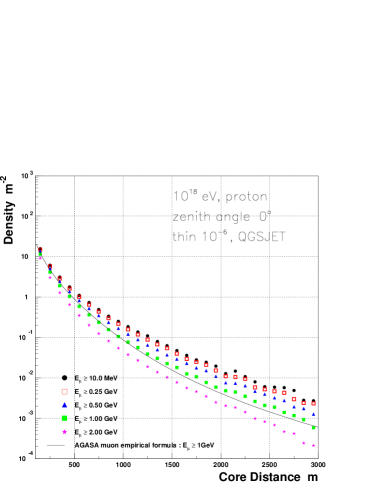
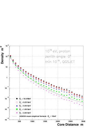
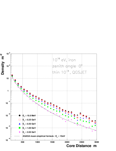
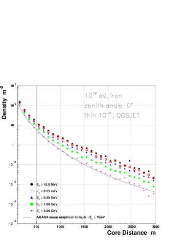
Figure 5: The lateral distributions of muons of cutoff energies above 10 MeV (top), 0.25 GeV, 0.5 GeV, 1.0 GeV and 2.0 GeV (bottom). QGSJET model. The thinning level is 10^-6. Upper figures are proton primaries and lower ones are iron. The incident energies are 10¹⁸ eV (left) and 10¹⁹ eV (right), respectively. Symbols as in Fig. 2.

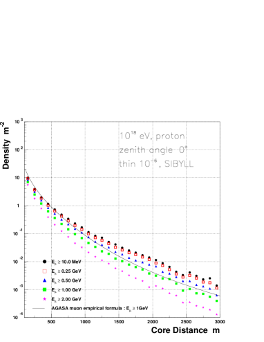
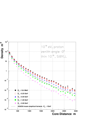
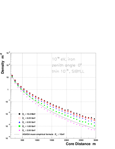
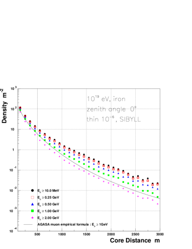
Figure 6: Same as Fig. 5, except for the hadronic interaction model is being SIBYLL.

It should be noted that the smaller muon number from the SIBYLL model relative to other interaction models used in CORSIKA has been pointed out in the 10¹⁴ eV $\sim$ 10¹⁵ eV region by Knapp et al. [29]. The slope of energy spectra of muons between 0.25 GeV and 1.5 GeV at 600 m from the core is similar irrespective of the QGSJET and the SIBYLL models and proton and iron primaries for 10¹⁹ eV. The experimental result [28] agrees well with the simulated ones except at 0.25 GeV, where we have in the experiment punch-through of the electromagnetic component into the muon detectors, even at 600 m from the core.

The relation of muon density above 1 GeV at 600 m from the core ($\rho_{\mu}(600)$) with the primary energy for three different combinations of simulation codes and interaction models is compared in Table 1. Here the slope $\alpha$ in $\rho_{\mu}\propto E^{\alpha}$ and the density at 10¹⁹ eV are listed. The results from the SIBYLL model with the MOCCA code [17] are also listed for comparison. Though the hadronic model is the same, there is about 10% difference in density between the results based on the two different simulation codes. The implications from this comparison will be made in Section 5.4.

Table 1: Comparison of slope and density at 10¹⁹ eV

Code	Model	Primary	Slope	$\rho_{\mu}$(600)	Note
				at 1019 eV
CORSIKA	QGSJET	proton	0.92	3.85
CORSIKA	QGSJET	iron	0.89	5.64
CORSIKA	SIBYLL	proton	0.88	2.39
CORSIKA	SIBYLL	iron	0.87	3.96
MOCCA	SIBYLL	proton	0.90	2.95	[17]
MOCCA	SIBYLL	iron	0.86	4.57	[17]

4.3 Charged particle density, $S_{0}$(600)

The relation of $S_{0}$(600) with the primary energy is examined for various conditions. $S_{0}$(600) does not depend on interaction model (QGSJET, SIBYLL) nor primary mass (proton, iron) within 20% which supports the previous simulations by Hillas et al. [5] and Dai et al. [6]. The $S_{0}$(600) vs. primary energy relation is almost linear, irrespective of primary mass (proton or iron) in case of QGSJET. However, $S_{0}$(600) $\sim E^{0.97}$ in case of SIBYLL. There are some differences between the simulated number of charged particles and the relation used at AGASA. The details will be discussed in Section 5.3.

4.4 Zenith angle dependence of charged particles

There is a zenith angle dependence of the lateral distribution of charged particles in the AGASA experiment and the slope parameter $\eta$ is expressed by Eq. 7 as a function of zenith angle. In Fig. 7, the lateral distribution of charged particles at a zenith angle of 39.7^∘ is shown for proton primaries of six primary energies. For the AGASA lateral distribution, $\eta=3.6$ and an attenuation length $\Lambda_{att}=500$ g cm^-2 are used. It is shown that the simulated results fit well to the experimental function, including the absolute values, independent of primary energy.

Figure 7: The lateral distributions of photons, electrons, muons and charged particles simulated at a zenith angle of 39.7^∘. The thinning level is 10^-6 and the cutoff energy of muons is 10 MeV and those of electrons and photons are 1 MeV. For drawing the AGASA lateral distribution, an attenuation length of 500 g cm^-2 is used and the change of $\eta$ with zenith angle is taken into account. Symbols as in Fig. 2.

Figure 8 shows the lateral distributions of charged particles at the four zenith angles $0^{\circ}$, 29.6^∘, 39.7^∘ and 51.3^∘ for proton (left) and for iron (right) primaries and for primary energies 10^18.5 eV and 10^19.5 eV, respectively. It should be noted that there are no differences in attenuation of charged particles with zenith angle between proton and iron primaries. The details will be discussed in Section 5.5.

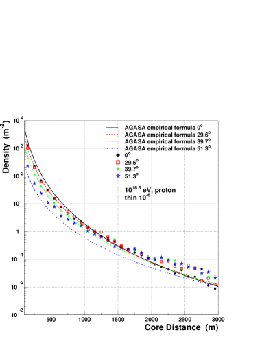
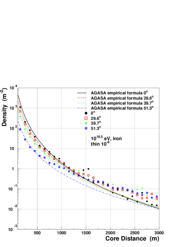
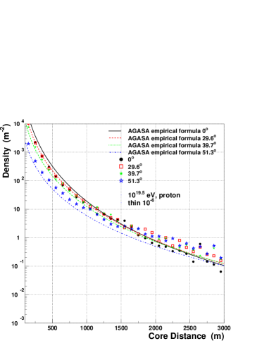
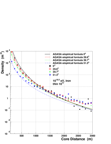
Figure 8: The lateral distributions of charged particles at four zenith angles 0^∘, 29.6^∘, 39.7^∘, and 51.3^∘ for primary energies 10^18.5 eV (top) and 10^19.5 eV (bottom). QGSJET model and cutoff energy of muons is 10 MeV and those of photons and electrons are 1.0 MeV. The left figure is for proton primary and the right one is for iron primary.

5 Discussion

The general features of the electromagnetic component and the low energy muons observed by AGASA can be well reproduced by CORSIKA simulation, except the slight differences in the absolute values. These discrepancies in absolute values between experiment and simulation are partly due to the assignment of primary energy, which depends on the definition of a single particle used in experiment and simulation. More remarkable discrepancies are the slope of $\rho_{\mu}$ vs. $S_{0}$(600) relation and zenith angle dependence $S_{\theta}$(600) for constant primary energy, which are shown in Fig. 12 and in Fig. 14, respectively. In the following we evaluate the simulated results with a similar definition of each observable as in the AGASA experiment.

5.1 Definition of density used in Akeno/AGASA experiment

In the AGASA experiment, a scintillator of 5 cm thickness is used to detect particles on the surface. The scintillator is placed inside an enclosure made of iron of 1.5 $\sim$ 2 mm thickness and the detector is in a hut whose roof is made of an iron plate of 0.4 mm thickness.

The definition of a single particle at the Akeno experiment (V₁) is the average of the pulse-height distribution of muons traversing a scintillator vertically [9]. V₁ is 10% larger than the peak value, since the distribution is not Gaussian, but subject to Landau fluctuations. If we use the peak value in pulse height distribution (PHD) of omnidirectional particles, the peak value V_ph is accidentally coincident with V₁ at Akeno level (V${}_{ph}\simeq$ V₁). To convert a density measured by a scintillator to an electron density corresponding to the calculated density by the NKG function [32], the density measured by scintillators and spark chambers at the Institute for Nuclear Study at Tokyo [16] is used at Akeno. This ratio is 1.1 between 10 m and 100 m from the core and hence the electron shower size (N_e) determined by the Akeno 1 km² array was reduced by 10% from the calculated N_e [9].

In AGASA a peak value V_pw in the pulse width distribution (PWD) of omnidirectional muons on a 5 cm scintillator is used as a single particle conventionally. The pulse width is obtained by discriminating a signal, which decays exponentially with a time constant of 10 $\mu$sec, at a constant level. V_pw is not equal to V_ph and is related to V_ph as :

$$V_{pw}=(V_{ph}+\sqrt{V_{ph}^{2}+\sigma^{2}})/2$$

where $\sigma$ is a full width at half maximum in PHD [33]. By putting V${}_{ph}=1.0$ and $\sigma=0.70$, we obtain V${}_{pw}=1.1$. A conventional value, V_pw, used at AGASA corresponds to 1.1$\times$V${}_{1}(\simeq 1.1\times$V_ph). That is V_pw corresponds to a measured density by spark chamber or the electron density, as far as the ratio of the density measured by scintillators and the spark chambers is 1.1.

Though there is a transition effect of the electromagnetic component in scintillator of 5 cm thickness within 30 m from the core [9], the density of charged particles as expressed in units of V₁ does not depend on the thickness of the scintillator above 30 m from the core as shown experimentally in Teshima et al. [34]. This can be understood since the radiation lengths of scintillator and air are very similar, so that the fraction of electrons at any depth in the scintillator changes only slowly as compared to air. This independence of thickness of scintillator has also been shown in the simulations of Cronin [14] and Kutter [15].

Assuming the 10% difference of scintillator density to spark chamber density at 600 m from the core, the density in units of V_pw (1.1 $\times$ V_ph) coincide with spark chamber density as described above and Eq. 1 was applied to deriving the AGASA energy spectrum.

5.2 Densities measured by scintillator of 5cm thickness

So far the AGASA group has used a factor 1.1 of scintillator density to spark chamber density which is determined within 100m from the core [16]. However, the factor has not yet been measured beyond 100 m from the core. In the following we discuss the lateral distribution of energy losses by photons, electrons and muons in 5cm scintillator in units of V_pw at Akeno level, taking into account the incident angles of electrons and photons far from the core, because the incident angles of electrons and photons on scintillator may not be vertical even for a vertical shower and the particles have some angular distribution.

In Fig. 9 the energy spectra of photons, electrons and muons are shown at core distances between 500 m and 800 m, simulated by CORSIKA. Many photons still remain at a zenith angle of 51.3^∘ ($\sec\theta=1.6$).

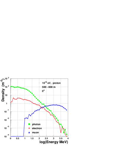
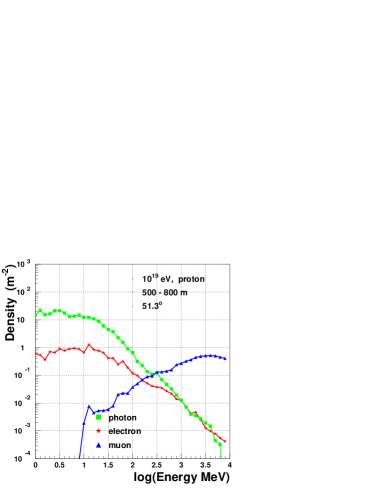
Figure 9: Energy spectra of photons, electrons and muons at core distance between 500 m and 800 m. The primary particle is a proton of 10¹⁹ eV. Zenith angles are 0^∘ (left) and 51^∘ (right).

Using CORSIKA, in a shower the incident angle of each particle to the surface is recorded, so that we can calculate the energy loss of each particle which is incident on the scintillator with various zenith angles. In the case of electrons and muons, only ionization loss is taken into account. The energy loss of photons is evaluated as follows. By dividing the scintillator in thin layers, the fraction of conversion to electrons in each layer is calculated using the photon attenuation length in water [35]. The energy loss of electron or electron/positron in the remaining layers for the fraction of photons is calculated. In this way the average energy loss of a single photon in a scintillator of various thicknesses is calculated as a function of the photon energy. Though the calculation process is simple, the result for a scintillator of 5 cm thickness agrees well with the Monte Carlo simulation results by Kutter [15]. The density of a shower of zenith angle $\theta$ is evaluated as the energy loss in scintillator of $5\times\sec\theta$ cm thickness (in units of V_pw) in an area of $1\times\cos\theta$ m².

In Fig. 10, the lateral distribution of energy deposit in scintillator of 5 cm thickness in units of V_pw ($\rho_{sc}$) is plotted by closed circles and compared with that of the experimental lateral distribution (dashed line). The simulated lateral distribution is flatter than the experimental one. $\rho_{sc}$ reflects the number of electrons near the core (up to about 200 m from the core), but becomes larger than the electron density with core distance. Though the agreement of $\rho_{sc}$(600) with the experimental $S_{0}$(600) is quite good, the difference of the lateral distribution of $\rho_{sc}$ from the experiment must be studied further.

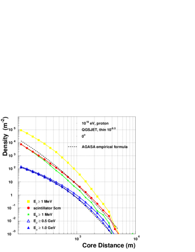
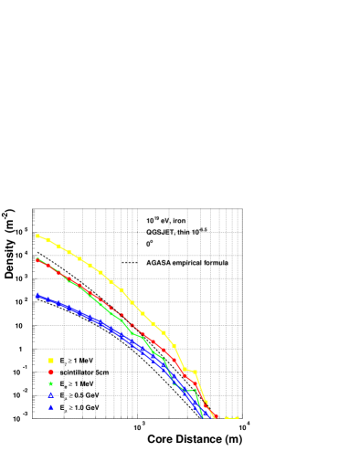
Figure 10: Lateral distribution of energy deposit in scintillator ($\bullet$) of 5 cm thickness ($\rho_{sc}$) in units of V_pw is compared with the experimental lateral distribution of AGASA. Those of electrons ($\geq$ 1 MeV), photons ($\geq$ 1 MeV), muons ($\geq$ 0.5 GeV) and muons ($\geq$ 1 GeV) are also shown. The left figure is proton primary and the right one iron.

5.3 Primary energy and $S_{0}$(600) relation evaluated by CORSIKA

In Table 2, the density of charged particles at 600 m from the core, $\rho_{ch}$(600), or the scintillator density of 5 cm thickness, $\rho_{sc}$(600), are listed for showers of 10¹⁹ eV of vertical incidence.

Table 2: Comparison of charged particle density ($\rho_{ch}$) or scintillator density in units of V₁ ($\rho_{sc}$) at 600 m from the core for showers of vertical incidence, 10¹⁹ eV and proton or iron primary.

Code	Model	Primary	Thinning	Threshold	$\rho_{ch}$(600) or	Note
			level	Eeγ (MeV)	$\rho_{sc}$(600) (m-2)
CORSIKA	QGSJET	proton	10-5	1.0	32.5
CORSIKA	QGSJET	proton	10-6	1.0	32.4
CORSIKA	QGSJET	proton	10-6	0.1	37.5
CORSIKA	QGSJET	proton	10-6	0.05	39.1
CORSIKA	QGSJET	iron	10-5	1.0	35.7
CORSIKA	QGSJET	iron	10-5	0.05	39.8
CORSIKA	SIBYLL	proton	10-6	1.0	30.4
CORSIKA	SIBYLL	iron	10-6	1.0	33.5
CORSIKA	QGSJET	proton	10-6	1.0	38.0
	-NKG			0	45.0
CORSIKA	QGSJET	proton	10-6	1.0	sci. 43.0
CORSIKA	QGSJET	iron	10-5	1.0	sci. 46.2
CORSIKA	SIBYLL	proton	10-6	1.0	sci. 38.2
CORSIKA	SIBYLL	iron	10-6	1.0	sci. 44.4
MOCCA	SIBYLL	proton		0.1	33.5	Cronin (1)
		iron		0.1	38.7	Cronin (1)
COSMOS	QCDjet	proton	10-5	0	50.0	Dai et al.(2)
	-NKG	CNO	10-5	0
		iron	10-5	0

⁽¹⁾ Simulation results made at Fermi Lab. using the SIBYLL interaction model with MOCCA simulation code (J.Cronin [14]).
⁽²⁾ Two dimensional simulation results made at ICRR with COSMOS by Dai et al. [6]. Photons and electrons of energies below the thinning energy level are connected to the NKG function in which the Molière length is used at 2 radiation lengths above the Akeno altitude.

The various combinations of simulation codes (CORSIKA, MOCCA), hadronic interaction models (QGSJET, SIBYLL), primary species (proton, iron), thinning levels and threshold energies of the electromagnetic components are compared.

In general, the difference of $\rho_{ch}$(600) due to the difference of simulation codes or hadronic interaction models is within 10% for the same cutoff energy of electromagnetic component. $\rho_{ch}$(600) depends on the cutoff energy of electromagnetic component. In the $S_{0}$(600) vs. energy relation by Dai et al. (Eq. 1), the electromagnetic component with energy of less than the thinning level is connected to the NKG function without cutoff energy for electrons and photons, and MU at 2 radiation lengths above the observation level is used. The result by CORSIKA simulated with the similar method is given in Table 2 as QGSJET-NKG. In case of CORSIKA, the relation is

$$E[\mbox{eV}]=2.2\times 10^{17}S_{0}(600)^{1.0}$$ (10)

and is about 10% larger than that by Dai et al.

The energy losses of photons, electrons and muons in scintillator of 5 cm thickness ($\rho_{sc}$(600)) in units of V_pw have been evaluated as described in the previous section by taking into account their incident angle to the scintillator and attenuation of low energy photons and electrons in the scintillator container and hut. The relation is drawn in Fig. 11 for proton and iron primaries. For the QGSJET hadronic interaction model we obtain

$$E[\mbox{eV}] = 2.07\times 10^{17}\rho_{sc}(600)^{1.03}\quad\mbox{for proton}$$ (11)

$$E[\mbox{eV}] = 2.24\times 10^{17}\rho_{sc}(600)^{1.00}\quad\mbox{for iron}$$ (12)

and for SIBYLL the relation reads

$$E[\mbox{eV}] = 2.30\times 10^{17}\rho_{sc}(600)^{1.03}\quad\mbox{for proton}$$ (13)

$$E[\mbox{eV}] = 2.19\times 10^{17}\rho_{sc}(600)^{1.01}\quad\mbox{for iron.}$$ (14)

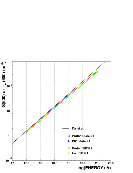
Figure 11: $S_{0}$(600) or $\rho_{sc}$(600) vs. energy relation estimated from the QGSJET and SIBYLL model for proton and iron primary.

Though there is a difference between proton and iron showers or QGSJET and SIBYLL, any combination assigns a higher energy than that by Eq. 1. The functions given by Eqs. 11, 12 and 14 intersect around $\rho_{sc}(600)=20\sim 30$, the combined relation may be written as

$$E[\mbox{eV}] = 5.65\times 10^{18}\left(\rho_{sc}(600)\over{25.0}\right)^{1.015},$$ (15)

by taking the average slope of the four equations. If we rewrite the above equation in similar form as Eq. 1, the following function may be used.

$$E[\mbox{eV}]=2.15\times 10^{17}S_{0}(600)^{1.015}.$$ (16)

Here we denoted $S_{0}$(600) instead of $\rho_{sc}$(600) as a scintillator density used in the experiment, since $S_{0}(600)\sim\rho_{sc}$(600) as described before. This equation means that the energy of the AGASA events must be increased by 14% at 10¹⁹ eV and 18% at 10²⁰ eV, if we evaluate the primary energy by CORSIKA.

5.4 Composition deduced from the muon component

The slope of the $\rho_{\mu}$(600) vs. energy relation measured by experiment is smaller than that in CORSIKA simulations. In Fig. 12 the $\rho_{\mu}$(600) vs. $S_{0}$(600) (or $\rho_{sc}$(600)) relation is shown. Since the relation $S_{0}$(600) vs. energy is almost linear irrespective of primary composition or interaction model used, the relation

$$\rho_{\mu}(600)=A\times S_{0}(600)^{b}$$

is similar to $\rho_{\mu}$(600) vs. energy relation and the parameter b is similar to $\alpha$ in Table 1.

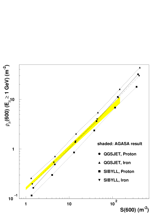
Figure 12: Comparison of experimental $\rho_{\mu}$ vs $S_{0}$(600) or $\rho_{ch}$ relation with that from CORSIKA simulation.

To explain the difference of slopes between experiment and simulation, Dawson et al. [17] favours a likely change in mass composition from heavy to light at energies above 10¹⁸ eV, as a supporting evidence of the change of mass composition claimed by the Fly’s Eye experiment [18]. The difficulty of their interpretation arises when the relation is applied to the energy region lower than 10¹⁷ eV. The $N_{\mu}$ vs $N_{e}$ relation of the Akeno result [26] is compared with the result of KASCADE [36] in Fig. 13 without any correction for each experiment. The empirical formula of Akeno at $\sec\theta=1.05$ is expressed by

$$N_{\mu}=(2.94\pm 0.14)\times 10^{5}\times(N_{e}/10^{7})^{0.76\pm 0.02}.$$ (17)

$N_{e}$ attenuates about a factor 1.5 from the Akeno level (920 g cm^-2) to the KASCADE level (1020 g cm^-2), while $N_{\mu}$ of the KASCADE experiment with the threshold energies of 2 GeV is expected to be smaller than that at Akeno of 1 GeV about a factor $1.2\sim 1.5$ [37]. Therefore such an agreement of the extrapolation of the absolute values from both experiments is well understood. The important result, however, is the agreement of the slopes of the $N_{\mu}$ vs. $N_{e}$ relation of both experiments in quite different energy regions.

Figure 13: $N_{\mu}$ vs. $N_{e}$ relation of the Akeno and the KASCADE experiments. The solid line represents Eq. 16 and the dashed one is its extrapolation.

Since in the higher energy region, $N_{e}$ can not be determined by AGASA, the $\rho_{\mu}$(600) vs. $S_{0}$(600) relation is used. The result at $\sec\theta=1.09$ [26] is expressed as

$$\rho_{\mu}(600)=(0.16\pm 0.01)\times S_{0}(600)^{0.82\pm 0.03}.$$ (18)

Taking into account the relation $S_{0}(600)\propto E_{0}\propto N_{e}^{0.9}$, the above equation coincides with Eq. 17 in the overlapping energy region [26]. Therefore the slope seems not to change from 10^14.5 eV to 10¹⁹ eV. If we take the absolute values of SIBYLL model as used in Dawson et al. [17] (refer to Fig. 4 of their paper), the composition becomes heavier than iron below 10¹⁷ eV. This conclusion demonstrates that it is important to compare the experimental results with simulations in as wide energy range as possible.

5.5 Attenuation of $S_{0}$(600) with zenith angle and the implication on the primary composition around 10¹⁹ eV

The $\rho_{sc}$(600) values are plotted in Fig. 14 as a function of atmospheric depth ($\sec\theta$) and connected with lines. The solid lines represent proton primaries and dotted ones are iron primaries. The experimental points of AGASA [38] are also plotted. These were obtained using the method of ‘equi-intensity cuts’ on the integral $\rho_{sc}$(600) spectra, based on the assumption that the flux of showers above a certain primary energy does not change with atmospheric depth. As shown in the figure the variation of $\rho_{sc}$(600) with zenith angle by CORSIKA (QGSJET) is similar to proton and iron primaries and is smaller than that of the experiment. If we take into account the error in $\rho_{ch}$(600) and zenith angle determination, this difference becomes larger, since flux of the observed $\rho_{ch}$(600) spectrum is increased by a factor of $\exp(\sigma^{2}(\gamma-1)^{2}/2)$, where $\sigma$ is the error in $\rho_{ch}$(600) determination in a logarithmic scale and $\gamma$ is the power index of the differential $\rho_{ch}$(600) spectrum [39].

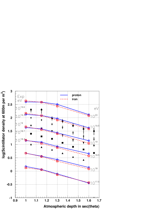
Figure 14: The variation of $\rho_{sc}$(600) with zenith angle. Solid lines are from protons and dotted are from iron (QGSJET model, thinning level 10^-6). Experimental points [20] correspond to 40, 20, 10, 5 and 2 $\times 10^{18}$ eV from top to bottom, respectively.

To examine the difference, the zenith angle variation of the electron density ($>1$ MeV) at 600 m from the core and the muon density ($>1$ GeV) at 600 m from the core are plotted in Fig. 15. The irregularities in the curves may be due to the statistical fluctuations of the limited number of simulated showers at each point and fitting errors to derive the density at 600 m. Within these uncertainties the attenuation with zenith angle by CORSIKA and that by Dai et al. agree with each other as in the left figure of Fig. 15. The difference of absolute values is partly due to the difference of cutoff energies as described before. Since the number of muons does not change with zenith angle and the number of muons in iron initiated showers are larger than that in proton showers as shown in the right figure of Fig. 15, the attenuation of $\rho_{ch}$(600), which consists of electrons above 1 MeV and muons above 10 MeV, does not depend on primary energy and composition.

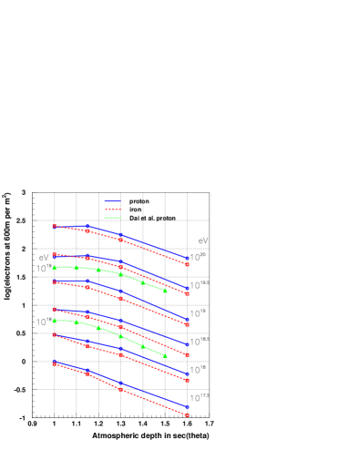
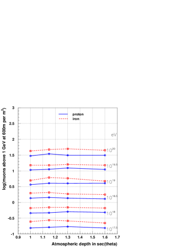
Figure 15: The variation of electron density at 600 m from the core with zenith angle (left) and that of muon density above 1 GeV at 600 m from the core (right). Solid lines are from proton primaries and dotted are from iron (QGSJET model, thinning level 10^-6 and cutoff energy of electrons are 1.0 MeV). Triangles connected with dotted lines are from Dai et al. [6] for primary protons of 10^18.0 eV and 10^19.0 eV, respectively.

As is described before, $S_{0}$(600) must be evaluated as $\rho_{sc}$(600), energy deposit in a scintillator in units of V_pw, at various zenith angles taking into account the increase of scintillator thickness with zenith angle. It is found that the attenuation of electromagnetic density with zenith angle is compensated with muon density and hence the attenuation of $\rho_{sc}$(600) with zenith angle is similar for proton and iron primaries in case of the QGSJET model. Therefore the muon density relative to the electromagnetic density, which is sensitive to the hadronic model, is an important quantity to compare with the experiment. Since the AGASA data have been increased considerably at the highest energy region compared to the one used in the Fig. 14, it may be better to await further comparisons for the publication of new experimental results.

6 Conclusion

An interpretation of AGASA data has been made by comparing them with results simulated with CORSIKA. Ten air showers for each of the primary energies 10^17.5 eV, 10^18.0 eV 10^18.5 eV, 10^19.0 eV 10^19.5 eV and 10^20.0 eV are simulated under each combination of the QGSJET or SIBYLL hadronic models and proton or iron primaries. General features of the electromagnetic component and low energy muons observed by AGASA can be well reproduced by CORSIKA. There are some discrepancies which must be studied in more detail to improve the agreement between the experiment and simulation. In the following some results implicated by the simulation related to the AGASA experiment are summarized.

The form of the lateral distribution of charged particles agrees well with the experimental one between a few hundred m and 2000 m from the core, irrespective of hadronic interaction model or composition and it does not depend on the primary energy simulated. Though the shape of the muon lateral distribution fits also the experiment, absolute values change with the hadronic interaction model and primary composition.

If we evaluate the density measured by scintillator of 5 cm thickness as $S_{0}$(600) by taking into account similar conditions as in the experiment, the conversion relation from $S_{0}$(600) to the primary energy can be written as

$$E[\mbox{eV}]=2.15\times 10^{17}S_{0}(600)^{1.015}.$$

This means that the energy assignment of the AGASA experiment is shifted to higher energies, if we estimate it using CORSIKA.

The slope of $\rho_{\mu}$ vs. $S_{0}$(600) relation in the experiment is flatter than that in simulations of any hadronic model and primary composition. The situation may not be changed even by taking into account the primary energy spectrum and fluctuations of $\rho_{\mu}$ and $S_{0}$(600). Since the slope seems to be constant in a wide primary energy range, we need to study this relation over a wide energy range. Otherwise the composition may be interpreted as heavier than iron or lighter than proton outside the narrow investigated energy region.

There is a disagreement of the attenuation length determined at AGASA and that by CORSIKA simulation, even if we take into account the particle incident angle to the scintillator. If we take into account the experimental error in zenith angle determination and $S_{0}$(600) determination, the disagreement increases. Since the experimental data used in the present analysis is still preliminary, we better wait for the publication of new experimental values for further discussions.

References

- [1] K. Greisen, Phys. Rev. Lett. 16 (1966) 748; Z.T. Zatsepin and V.A. Kuzmin, Pisma Zh. Eksp. Teor. Fiz. 4 (1966) 144.
- [2] D. Bird et al., Astrophys. J. 441 (1995) 144.
- [3] N. Hayashida et al., Phys. Rev. Lett. 73 (1994) 3491.
- [4] M. Takeda et al., Phys. Rev. Lett. 81 (1998) 1163; Astrophys. J. 522 (1999) 225.
- [5] A.M. Hillas et al., Proc. 12th ICRC (Hobart), 3 (1971) 1001.
- [6] H.Y. Dai et al., J. Phys. G: Nucl. Phys. 14 (1988) 793.
- [7] K. Kasahara, S. Torii and T. Yuda, Proc. 16th ICRC (Kyoto) 13 (1979) 70.
- [8] L.K. Ding et al., Proc. Int. Symp. on Cosmic Rays and Particle Physics (ed. by T.Yuda, Inst. for Cosmic Ray Research, University of Tokyo) (1984) 142.
- [9] M. Nagano et al., J. Phys. Soc. Japan 53 (1984) 1667.
- [10] M.A. Lawrence, R.J.O. Reid and A.A. Watson, J. Phys. G: Nucl. Phys. 17 (1991) 733.
- [11] B.N. Afanasiev et al., Proc. Tokyo Workshop on Techniques for the Study of the Extremely High Energy Cosmic Rays (ed. by M.Nagano, Inst. for Cosmic Ray Research, University of Tokyo) (1993) 35.
- [12] D.J. Bird et al., Astrophys. J. 424 (1994) 491.
- [13] M. Sakaki et al., Proc. 25th ICRC (Durban) 5 (1997) 217.
- [14] J.W. Cronin, GAP-97-034 (Auger Technical Note) (1997).
- [15] T. Kutter, GAP-98-048 (Auger Technical Note) (1998).
- [16] S. Shibata et al., Proc. 9th ICRC (London) 2 (1965) 672.
- [17] B. Dawson, R. Meyhandan and K.R. Simpson, Astroparticle Phys. 9 (1998) 331.
- [18] T.K. Gaisser et al., Phys. Rev. D 47 (1993) 1919.
- [19] M. Nagano et al., J. Phys. G: Nucl. Part. Phys. 18 (1992) 423.
- [20] S. Yoshida et al., J. Phys. G: Nucl. Phys. 20 (1994) 651.
- [21] D. Heck et al., FZKA6019 (Forschungszentrum Karlsruhe) (1998).
- [22] D. Heck and J. Knapp, FZKA6097 (Forschungszentrum Karlsruhe) (1998).
- [23] N. Chiba et al., Nucl. Instrum. and Methods A311 (1992) 338.
- [24] H. Ohoka et al., Nucl. Instrum. and Methods A385 (1996) 268.
- [25] N. Sakaki et al., Proc. 26th ICRC (Salt Lake City) 1 (1999) 361.
- [26] N. Hayashida et al., J. Phys. G: Nucl. Phys. 21 (1995) 1101.
- [27] T. Doi et al., Proc. 24th ICRC (Rome) 2 (1995) 764.
- [28] Y. Matsubara et al., Proc. 19th ICRC (La Jolla) 7 (1985) 119.
- [29] J. Knapp, D. Heck and G. Schatz, FZKA5828 (Forschungszentrum Karlsruhe) (1996).
- [30] N.N. Kalmykov and S.S. Ostapchenko, Yad. Fiz 56 (1993) 105.
- [31] R.S. Fletcher et al., Phys. Rev. D 50 (1994) 5710.
- [32] K. Greisen, Prog. Cosmic Ray Physics, 3rd. (ed. by J.G. Wilson) (1956) p.27.
- [33] Akeno Internal Manual, (1980) unpublished.
- [34] M. Teshima et al., J. Phys. G: Nucl. Phys. 12 (1995) 1097.
- [35] R.M. Barnett et al., Phys. Rev. D 54 (1996) 1.
- [36] H. Leibrock, L. Haungs and H. Rebel, unpublished report of Forschungszentrum Karlsruhe (1998).
- [37] K. Greisen, Ann. Rev. Nucl. Sci. 10 (1960) p.63.
- [38] N. Hayashida et al., Proc. 25th ICRC (Durban) 4 (1997) 145.
- [39] V.S. Murzin, Proc. 9th ICRC (London) 2 (1965) 872.