Lensing effects in an inhomogeneous universe

Abstract

Recently, Holz & Wald have presented a new method for determining gravitational lensing effects on, e.g., supernova luminosity versus redshift measurements in inhomogeneous universes. In this paper, their method is generalized in several ways: First, the matter content is allowed to consist of several different types of fluids, possibly with non-vanishing pressure. Second, besides lensing by simple point masses and singular isothermal spheres, the more realistic halo dark matter distribution proposed by Navarro, Frenk & White (NFW), based on N-body simulation results, is treated. We discuss various aspects of the accuracy of the method, such as luminosity corrections, and statistics, for multiple images. We find in agreement with other recent work that a large sample of supernovae at large redshift could be used to extract gross features of the mass distribution of the lensing dark matter halos, such as the existence of a large number of point-like objects. The results for the isothermal sphere and the NFW model are, however, very similar if normalized to the observed luminosity distribution of galaxies. We give convenient analytical fitting formulas for our computed lensing probabilites as a function of magnification, for several redshifts.
Key words: cosmology: theory, gravitational lensing, dark matter – galaxies: halos

1 Introduction

Ever since the foundation of modern cosmology based on general relativity, there have been attempts to determine the cosmological parameters of our universe. Gravitational lensing has been recognized as one of several such tools. For example, the results of radio surveys for gravitational lenses have recently been used to place significant constraints on cosmological models (Falco et al. radiolens (1998)). It has also been realised that observations of supernovae at high redshift can be used for this purpose (Goobar & Perlmutter art:GoobarPerlmutter1995 (1995)), in particular for determining the value of the cosmological constant. In fact, several collaborations with this in mind are in progress, and the first sets of data show an intriguing hint of a non-vanishing cosmological constant in a universe consistent with having a flat geometry (see, e.g., Riess et al. art:Riess-et-al1998 (1998); Perlmutter et al. art:Perlmutter-et-al1999 (1999)). Although the two groups which have published results mutually agree on the best-fit parameters, it is important to note that the effects of geometry are small (on the order of half a magnitude), and the need to go to even higher redshift to get larger effects is obvious. When observing such distant sources, at redshift greater than unity, it is necessary to estimate the effects of lensing due to inhomogeneities in the matter distribution. This will be of growing importance when supernovae at very high redshifts become accessible, e.g., with NGST, the Next Generation Space Telescope (Miralda-Escudé & Rees MI97 (1997); Dahlén & Fransson DA99 (1999)) or with the dedicated supernova search satellite, SNAP (Perlmutter et al., private communication).

The literature on gravitational lensing is quite rich. Much of the history and developments up to the early 1990s can be found in the excellent textbook by Schneider, Ehlers & Falco (book:Schneider (1992)). A new method for examining lensing effects has recently been proposed by Holz & Wald (art:HolzWald1998 (1998); HW), one which has the virtue of lending itself easily to numerical calculations. In that work it is also shown that given a large and deep enough sample of standard candle supernovae, one may in principle distinguish between different matter distributions in the galactic halos responsible for the lensing. In particular the case of point masses gives a quite different distribution of magnifications (or de-magnifications) compared to the case of singular isothermal spheres (see also Metcalf & Silk metcalf (1999)).

The method of HW can be summarized as follows: First, a Friedmann-Lemaître (FL) background geometry is selected. Inhomogeneities are accounted for by specifying a matter distribution in cells which have an average energy density equal to that of the underlying FL model. Following the history of observed light from a distant source, a light ray is traced backwards to the desired redshift by being sent through a series of cells, each time with a randomly selected impact parameter with respect to the matter distribution in the cell. Between each cell, the FL background is used to update the scale factor and the expansion rate. By using Monte Carlo techniques to trace a large number of such light rays, statistics for the apparent luminosity of an ensemble of sources at a given redshift is obtained.

The purpose of this paper is to generalize the method of HW in a number of ways and to investigate some issues related to the different lensing signatures in the luminosity distribution of supernovae caused by different mass distributions of the intervening lens population. The outline is as follows. In Sect. 2 it is demonstrated how the HW method can be generalized from matter in dust form to perfect fluids with pressure. Sect. 3 is concerned with the interpretation of results as probability distributions. Sect. 4 presents the geodesic deviation and in Sect. 5, we summarize and discuss some of the conceptual issues in the analysis of HW. In Sect. 6, we include the possibility of using the more realistic halo matter distribution proposed by Navarro et al. (art:NFW (1997); NFW) based on their N-body simulation results, and in Sect. 7 we discuss the mass distribution of lensing galaxies. By using realistic density profiles and mass distributions of dark matter halos, we can obtain high accuracy results on gravitational lensing without the need of using the extensive full data sets of N-body simulations, as in some other methods (Wambsganss et al. cen (1998); Premadi et al. premadi (1998); Jain et al. jain (1999)). One strength of our ray-tracing Monte Carlo method is further that it can be continuously refined as more observational information, e.g., on galaxy distributions is obtained. Also, effects such as absorption by dust and other possibly $z$-dependent effects can be straightforwardly added to the algorithm. In Sect. 8, some results from the generalizations of the method of HW are presented as luminosity distributions. In Sect. 9, we investigate some limitations of the numerical implementation of the method and in Sect. 10, we discuss multiple images. Sect. 11 investigates different consistency checks, Sect. 12 contains convenient analytical fits to our numerical results and the paper is concluded with a discussion in Sect. 13.

2 Cosmological model

The starting point of HW is a Newtonianly perturbed FL universe. The line element of Robertson-Walker form is then

$$ds^{2}=-(1+2\phi)dt^{2}+(1-2\phi)a^{2}(t)dl^{2}_{k},$$ (1)

where $a$ is the scale factor, and $dl^{2}_{k}$ is a constant-curvature three-geometry, for which $k\in\{0,\pm 1\}$ indicates the sign of the curvature. (We use geometrized units such that $G=c=1$). The perturbation $\phi$ is assumed to satisfy a number of properties that will be employed when determining dominant terms. Firstly, $|\phi|\ll 1$, reflecting that $\phi$ indeed is a perturbation. Secondly, inhomogeneities are assumed to be significant, so that $\partial\phi/\partial t$ is small compared to spatial derivatives. Thirdly, second-order spatial derivatives will be assumed to dominate over products of first-order ones (e.g., $(\partial_{x}\phi)^{2}\ll|\partial_{xx}\phi|$). In this paper, we have generalized the treatment of HW so that the matter content of the model can be taken to be a number of perfect fluids:

$$T_{ab}=\sum_{i}\rho_{i}u_{a}u_{b}+p_{i}(u_{a}u_{b}+g_{ab}),$$ (2)

where $T_{ab}$ is the stress-energy tensor, $\rho_{i}$ is the energy density, $p_{i}$ the pressure of fluid $i$, $u^{a}$ is the (normalized) fluid four-velocity, and $g_{ab}$ is the metric corresponding to the line element (1). Cosmologically reasonable equations of state are linear barotropic ones: $p_{i}=\alpha_{i}\rho_{i}$. In this paper, the $\alpha_{i}$’s are constants with $-1\leq\alpha_{i}\leq 0$. However, it is straightforward to allow for the equations of state to evolve with redshift, i.e., $\alpha_{i}=\alpha_{i}(z)$.

HW considered dust models with a cosmological constant, which corresponds to a two-fluid model, the first fluid having $\alpha_{1}=0$, and the second fluid homogeneously distributed with $\alpha_{2}=-1$ and $\Lambda=8\pi\rho_{2}$. The field equations, corresponding to Eqs. (HW7,8), become
The Friedmann equation:

$$3\left(\frac{\dot{a}}{a}\right)^{2}=3H^{2}=8\pi\sum_{i}\rho_{i}-\frac{3k}{a^{2}}-2\nabla^{2}\phi,$$ (3)

The Raychaudhuri equation:

$$3\frac{\ddot{a}}{a}=-3qH^{2}=-4\pi\sum_{i}(\rho_{i}+3p_{i})+\nabla^{2}\phi,$$ (4)

where the definitions of the Hubble scalar $H$ and deceleration parameter $q$ have been made explicit, and where $\nabla^{2}$ denotes the spatial projection of contracted covariant derivatives. The pressure does not enter the Friedmann equation, i.e., the Hubble scalar is entirely given by the energy densities and the curvature. The deceleration, on the other hand, is affected by the presence of pressure. Comparing the above field equations with the field equations for the corresponding FL background (with averaged densities and pressures $\bar{\rho}_{i}$, $\bar{p}_{i}$) it can be shown [Eq. (HW11)] that $\phi$ satisfies a Poisson equation $\nabla^{2}\phi=4\pi\sum_{i}\delta\rho_{i}$, where $\delta\rho_{i}=\rho_{i}-\bar{\rho}_{i}$, while $\delta p_{i}=p_{i}-\bar{p}_{i}$ vanishes. Thus, the pressures result in homogeneous contributions, and the specification of an equation of state only makes sense in terms of the averaged energy density: $p_{i}=\bar{p}_{i}=\alpha_{i}\bar{\rho}_{i}$.

From the field equations for the background model follows
The energy conservation equation:

$$\sum_{i}\dot{\bar{\rho}}_{i}+3(\bar{\rho}_{i}+\bar{p}_{i})H=0.$$ (5)

If the fluids are assumed to couple only to gravity, they will be separately conserved, and each component in the sum of Eq. (5) vanishes. Note that it is only for dust ($p=0$) that the mass within a volume co-moving with the Hubble flow is constant ($\bar{\rho}\propto a^{-3}$). For other types of matter, the mass varies with time because of the work done by the pressure. Also note that $p=-\rho$ results in a constant energy density. Thus, a homogeneously distributed fluid with $p=-\rho$ is equivalent to a cosmological constant, or in terms of quantum field models, to vacuum energy. It is convenient to introduce density parameters

$$\Omega_{i}=8\pi\bar{\rho}_{i}/3H^{2},$$ (6)

which depend on time and therefore on redshift. Assuming the above discussed equations of state the time dependence is governed by the following set of conservation equations (see, e.g., Goliath & Ellis art:GoliathEllis1999 (1999))

$$\dot{\Omega}_{i}=\left[2q-(3\alpha_{i}+1)\right]\Omega_{i}H.$$ (7)

HW proceed by performing a number of coordinate transformations to co-moving coordinates on isotropic form, Eq. (HW16). The inclusion of pressure results in a modification of this line element:

$$ds^{2}= - \left[1+2\Phi+4\pi R^{2}\sum_{i}p_{i}\right]dT^{2}$$ (8)

$$+ \left[1-2\Phi\right](dX^{2}+dY^{2}+dZ^{2}),$$

where $R^{2}\approx X^{2}+Y^{2}+Z^{2}$, and the effective potential

$$\Phi=\phi+\frac{2\pi R^{2}}{3}\sum_{i}\rho_{i}$$ (9)

satisfies the Poisson equation

$$\nabla^{2}\Phi=4\pi\sum_{i}\rho_{i}.$$ (10)

The lookback time of an event at redshift $z_{1}$ is the time difference (with respect to the coordinate $t$) between the event and the present. By using $1+z=a_{0}/a$, we get a relation between the lookback time and the redshift for a FL universe:

$$\Delta t=\int_{a_{1}}^{a_{0}}\frac{da}{\dot{a}}=\int_{0}^{z_{1}}\frac{dz}{(1+z)H(z)}.$$ (11)

To obtain $H(z)$, the Friedmann equation, Eq. (3), is expressed in terms of redshift and the present densities $\rho_{0i}$. To do so, first note that the energy conservation equation, Eq. (5), together with the equation of state gives

$$\bar{\rho}_{i}=\bar{\rho}_{0i}\left(\frac{a}{a_{0}}\right)^{-3(1+\alpha_{i})}=\bar{\rho}_{0i}(1+z)^{3(1+\alpha_{i})}.$$ (12)

The Hubble scalar can then be expressed

$$H(z)=H_{0}\sqrt{\sum_{i}\Omega_{0i}(1+z)^{3(1+\alpha_{i})}+\Omega_{0k}(1+z)^{2}},$$ (13)

where we introduced the curvature density parameter

$$\Omega_{0k}=1-\sum_{i}\Omega_{0i}=-\frac{k}{H_{0}^{2}a_{0}^{2}}.$$ (14)

The luminosity distance to the event at redshift $z_{1}$ is given by a similar expression (see, e.g., Bergström & Goobar book:BergstromGoobar1999 (1999))

$$d_{L} = a_{0}(1+z)\ \mbox{\Large{\it f}}\,\left(\frac{1}{a_{0}}\int_{0}^{z_{1}}\frac{dz}{H(z)}\right),$$ (15)

$$f(x) = \left\{\begin{array}[]{ll}\sin(x),&k=1\\ x,&k=0,\\ \sinh(x),&k=-1\\ \end{array}\right.$$ (19)

Note that, when $k=\pm 1$, the present scale factor can be expressed [using (14)] as $a_{0}=(H_{0}\sqrt{|\Omega_{0k}|})^{-1}$.

3 Area vs. magnification and statistical weighting

Consider a narrow (strictly speaking; infinitesimal) ray bundle connecting a source and an observer as depicted in Fig. 1. The ray bundle can be focused either at the source or the observer. The relevant quantity when determining luminosity distances is the ratio of the area of a beam and the solid angle it subtends. Of course, the smaller the distance, the brighter the source.

Figure 1: Geometry of ray bundle.

In the method of HW, a beam focused at the observer with infinitesimal $\delta\Omega$ is integrated backwards using the geodesic deviation equation, and the resulting area at the source sphere is considered. In the lower panel of Fig. 1, the beam has undergone additional focusing. A finite aperture at the observer will detect light from a larger $\delta\Omega$ of an isotropically emitting source, and a finite source will subtend a larger solid angle on the sky. Since surface brightness is conserved, the source will be magnified. The magnification, $\mu$, is defined as the ratio of the observed flux and the flux of the corresponding image in absence of any additional focusing.

$$\mu=\frac{\delta\Omega}{\delta\Omega_{0}}$$ (20)

where $\delta\Omega_{0}$ denotes the solid angle subtended by the source in absence of lenses. Hence the magnification will be proportional to the inverse of the area of the beam. In absence of any lenses, the ray bundle will have an area corresponding to the so called empty-beam area (see Sect. 4), and we will therefore define the magnification as

$$\mu=\frac{A_{\rm empty}}{A}.$$ (21)

For further reference, see Schneider, Ehlers & Falco (book:Schneider (1992)).

As noted in HW, some care is needed when interpreting results as probability distributions. This is due to the fact that individual ray bundles do not correspond to random source positions. This is illustrated in the left panel of Fig. 2 where we consider the situation of a ray bundle originating from an observer at $z=0$ at the center of a source sphere at some fixed redshift.

Figure 2: Different ray bundles with constant $\delta\Omega$

From the right panel of Fig. 2 we see that focused beams sample a smaller fraction of the source sphere.

Since the fraction of the source sphere being sampled by a beam is proportional to the area of the beam, i.e., inversely proportional to the magnification, magnified sources will be overrepresented if not compensated for. In HW, this is done by convoluting the obtained probability distribution, $n_{0}(A)$, with a factor proportional to $A$, thus obtaining a new distribution $n(A)\propto A\,n_{0}(A)$. The method we use is very similar in that we designate a probability, proportional to the area of the ray bundle, to keep every event. The advantage of this rejection method is that each selected event represents a statistically “real” event.

Further discussions of the statistical weight given to random line-of-sights can be found in Ehlers & Schneider (EH86 (1986)).

4 Geodesic deviation

The geodesic deviation equation for a light ray is (see, e.g., Wald book:Wald1984 (1984))

$$\frac{d^{2}\xi^{a}}{d\lambda^{2}} = -\Delta^{a}\!_{b}\xi^{b},$$ (22)

$$\Delta_{ab} = R_{cadb}k^{c}k^{d},$$ (23)

where $\xi^{a}$ is the deviation vector and $k^{a}$ is a null vector tangent to the light ray. The affine parameter $\lambda$ is a parametrization along the light ray given by $\omega d\lambda=dt$, where $\omega$ is the frequency of the photons in the beam. It is instructive to calculate the deviation in an exact (homogeneous) FL universe, analogous to Eq. (HW21):

$$\frac{d^{2}\xi^{\alpha}}{d\lambda^{2}}=-4\pi\omega^{2}\sum_{i}(\rho_{i}+p_{i})\xi^{\alpha}.$$ (24)

Thus, the pressure will cause additional focusing of the light beam. Note that a cosmological constant, which corresponds to $p=-\rho$, does not affect the deviation.

To derive the deviation experienced when propagating through a cell in the inhomogeneous model, HW start by writing the deviation equation in terms of a $2\times 2$ matrix ${\cal A}^{\alpha}\!_{\beta}$, such that

$$\frac{d^{2}{\cal A}^{\alpha}\!_{\beta}}{d\lambda^{2}}=-\Delta^{\alpha}\!_{\gamma}{\cal A}^{\gamma}\!_{\beta},$$ (25)

where $\alpha,\beta\in\{X,Y\}$ (HW28). The properties of the geodesic deviation are contained in ${\cal A}^{\alpha}\!_{\beta}$. For example, the area (with orientation) of the beam is given by $\det{\cal A}$. In the case of the homogeneous background Friedmann-Lemaître cosmology, we denote the corresponding reference area $A_{\rm FL}$, which will of course depend on the redshift, but also on the cosmological parameters of the FL background model. Also, the area of a light beam that propagates without encountering any matter will be denoted $A_{\rm empty}$. Sometimes $A_{\rm FL}$ and $A_{\rm empty}$ are referred to as the filled-beam and empty-beam areas, respectively.

The deviation equation, Eq. (25), can now be written as a set of difference equations (HW35,36)

$$({\cal A}^{\alpha}\!_{\beta})_{1} =({\cal A}^{\alpha}\!_{\beta})_{0}+\Delta\lambda(d{\cal A}^{\alpha}\!_{\beta}/d\lambda)_{0},$$ (26)

$$(d{\cal A}^{\alpha}\!_{\beta}/d\lambda)_{1} =(d{\cal A}^{\alpha}\!_{\beta}/d\lambda)_{0}-\omega J^{\alpha}\!_{\gamma}({\cal A}^{\gamma}\!_{\beta})_{0},$$ (27)

with

$$J^{\alpha}\!_{\beta}=\frac{1}{\omega}\int_{c}d\lambda\Delta^{\alpha}\!_{\beta},$$ (28)

where the integration is along a straight line through the cell. Next, $\Delta_{\alpha\beta}$ is calculated from the line element Eq. (8)

$$\Delta_{\alpha\beta}\!=\!\omega^{2}\!\left\{\!2\partial_{\alpha}\partial_{\beta}\Phi\!+\!\left[Z^{a}\partial_{a}(Z^{b}\partial_{b}\Phi)\!+\!4\pi\!\sum_{i}p_{i}\right]\!\eta_{\alpha\beta}\!\right\},$$ (29)

where $\eta_{ab}$ is the Minkowski metric associated with the coordinates $(T,X,Y,Z)$. Thus, with non-vanishing pressure, there will be an additional contribution in $J^{\alpha}\!_{\beta}$ that takes the form

$$J^{\alpha}_{p}\!{}_{\beta}=\left(\sum_{i}J_{p_{i}}\right)\,\delta^{\alpha}\!_{\beta},$$ (30)

with

$$J_{p_{i}} = 4\pi\omega p_{i}\int_{c}d\lambda$$ (31)

$$= 4\pi p_{i}\int_{c}dZ$$

$$= 4\pi p_{i}\,2R_{c}\sqrt{1-\frac{b^{2}}{R_{c}^{2}}}$$

$$= \frac{6p_{i}V_{c}}{R_{c}^{2}}\sqrt{1-\frac{b^{2}}{R_{c}^{2}}},$$

where $b$ is an impact parameter, and $R_{c}$ and $V_{c}$ are the radius and volume of the cell, respectively. Assuming linear barotropic equations of state, $p_{i}=\alpha_{i}\bar{\rho}_{i}$, Eq. (31) becomes

$$J_{p_{i}}=\alpha_{i}\frac{6M_{i}}{R_{c}^{2}}\sqrt{1-\frac{b^{2}}{R_{c}^{2}}},$$ (32)

where $M_{i}$ is the mass of matter component $i$ in the cell.

Let us now examine the above result for the filled-beam case. Eq. (HW39) gives the quantity $J^{\alpha}\!_{\beta}$ for matter uniformly distributed in a ball of radius $d$ at the center of a cell of radius $R_{c}$. Setting $d=R_{c}$ in this equation, and adding our derived pressure contribution $\sum_{i}J_{p_{i}}\delta^{\alpha}\!_{\beta}$ to this yields

$$(J^{\rm FL})^{X}\!_{X} = (J^{\rm FL})^{Y}\!_{Y}=\sum_{i}(1+\alpha_{i})\frac{6M_{i}}{R_{c}^{2}}\sqrt{1-\frac{b^{2}}{R_{c}^{2}}},$$

$$(J^{\rm FL})^{X}\!_{Y} = (J^{\rm FL})^{Y}\!_{X}=0,$$ (33)

from which it is seen that a cosmological constant ($\alpha=-1$) does not contribute, in consistency with Eq. (24).

As an interesting example, consider a flat cosmological model in which ordinary matter ($\alpha=0$) constitutes only 10 % of the total matter content, i.e., $\Omega_{M}=0.1$, while the rest is made up of some homogeneously distributed “X-matter” with $\Omega_{X}=0.9$. The ordinary matter is assumed to be in the form of point masses (we will return later to more realistic mass distributions). For this cosmology, Garnavich et al. (Garnavich (1998)) have put an upper limit on the parameter of the equation of state for an X-matter component using Type Ia supernova data. Their limit is $\alpha_{X}<-0.60$ at 95 % confidence level. Similarly, the Supernova Cosmology Project (Perlmutter et al. art:Perlmutter-et-al1999 (1999)) has deduced a limit of $\alpha_{X}<-0.44$ (95 % cl) for any value of $\Omega_{M}$.

In Fig. 3, we compare the cases of $\alpha_{X}=-1$, corresponding to a cosmological constant, $\alpha_{X}=-2/3$, which may either arise from “quintessence” (i.e., a slowly evolving scalar field) (Wang et al. steinhardt (1999)) or from a domain wall network (Battye et al. spergel (1999)). For reference, we also show the result for $\alpha_{X}=0$, corresponding to dust (i.e., equivalent to an Einstein–de Sitter model with $\Omega_{M}=1$, of which 90 % is homogeneously distributed). The choice of $\Omega_{M}=0.1$ is made to allow for a direct comparison of the curve corresponding to $\alpha_{X}=-1$ in Fig. 3 with Fig. 7 in HW, with which it agrees well.

Note that the normalization differs between the three cases since $A_{\rm FL}$ depends on the cosmology. Nevertheless, from the slope of the curves, one can conclude that lensing effects become more prominent for large negative $\alpha_{X}$. This is not what one would expect from studying the geodesic deviation equation, Eq. (24), since negative pressure causes less focusing of a beam. However, for negative $\alpha_{X}$, distances will get larger for a fixed redshift, which means a larger number of lenses between the source and the observer (see, e.g., Turner TU90 (1990)).

Figure 3: Beam areas normalized to the filled-beam value of the underlying Friedmann-Lemaître model $A_{\rm FL}$ for 10 000 sources at redshift $z=3$ in a $\Omega_{M}=0.1$, $\Omega_{X}=0.9$ universe. The matter is assumed to be in the form of point masses, and results for the equation of state coefficient $\alpha_{X}$ of the homogeneous $X$ component having the value $0$ (solid line), $-2/3$ (long-dashed line) and $-1$ (short-dashed line) are shown. The horizontal scale gives cumulative percentage of beams having an area less than a given value. Negative areas correspond to secondary images.

5 Summary of the properties of the lensing model

The method of Holz & Wald (art:HolzWald1998 (1998)) which we adopt has a number of properties, which we summarize and comment upon here:

• Local nature of lensing
  If $\phi$ is small within distances much smaller than the Hubble radius $R_{H}=H^{-1}$, then the curvature (and thereby the lensing effects) is determined locally within $R_{H}$. Likewise, if we assume that there is no strong correlation on scales greater than a clustering scale $R$, it follows that the curvature is determined locally within $R$.

• Relevant scales
  The question now is what relevant clustering scale to use. HW find it convenient to employ the typical separation between galaxies, and argue that galaxy clustering should have a negligible effect on magnification, as shown in some of their simulations. They also argue that the smallest relevant scale for matter clumping is of the order $10^{-3}M_{\odot}$, since objects smaller than that would not give a coherent lensing effect over the angular size of most of the interesting sources.

• Generality
  For the case of point masses, HW demonstrate that their results are fairly insensitive to the size of individual point masses. Furthermore, their results are rather insensitive to clustering. This is tested by cutting out a tube in a uniform matter distribution and distributing “stars” within this tube.

• Largest effects
  Based upon their results, HW conjecture that randomly distributed point masses should cause the largest lensing effects of all possible mass distributions for a given average mass density. Note that the point-mass case corresponds to the limit in which all matter clumps lie well within their Einstein radii [see Eq. (34)].

Comment on relevant scales:
The Einstein radius is a characteristic length scale in the lens plane given by

$$\xi_{0}=\sqrt{2R_{\rm Schw}\frac{D_{d}D_{ds}}{D_{s}}},$$ (34)

where $R_{\rm Schw}=2M$ is the Schwarzschild radius of the lens and $D_{ds}$, $D_{d}$ and $D_{s}$ are angular diameter distances between lens and source, observer and lens, and observer and source, respectively. The corresponding length scale in the source plane, $\eta_{0}$, is

$$\eta_{0}=\frac{D_{s}}{D_{d}}\xi_{0}=\sqrt{2R_{\rm Schw}\frac{D_{s}D_{ds}}{D_{d}}}.$$ (35)

For lensing to be important, the source size, $l$, has to be smaller than the length scale $\eta_{0}$ introduced by a point mass lens, $l<\eta_{0}$. The source size of a type I supernova is $\sim 10^{15}$ cm at maximum luminosity. Putting the source at $z=1$ and the lens at $z=0.5$ in a flat universe with $\Omega_{M}=0.3$ and the dimensionless Hubble parameter $h=0.65$, we obtain

$$M>10^{-4}M_{\odot},$$ (36)

i.e., only compact objects with $M>10^{-4}M_{\odot}$ should be of importance through microlensing of supernovae.

6 The Navarro-Frenk-White distribution

The work of HW has as a first treatment been concerned with the $J^{\alpha}\!_{\beta}$ expressions for idealised cases like point sources; singular, truncated isothermal spheres (SIS); uniform spheres; and uniform cylinders. However, another often-used matter distribution is the one based on the results of detailed N-body simulations of structure formation given by Navarro et al. (art:NFW (1997)). They parametrize the density profile by

$$\rho(r)=\frac{\rho_{\rm crit}\delta_{c}}{(r/R_{s})^{\gamma}[1+(r/R_{s})^{1/\delta}]^{(\beta-\gamma)\delta}},$$ (37)

where $\rho_{\rm crit}=3H^{2}/8\pi$ is the critical density, $\delta_{c}$ is a dimensionless density parameter and $R_{s}$ is a characteristic radius.

NFW found that halos found in N-body simulations ranging in mass from dwarf galaxies to rich galaxy clusters can be fit by Eq. (37) with $\gamma=1$, $\beta=3$, $\delta=1$. The potential for this density profile is given by

$$\Phi(r)=-4\pi\rho_{\rm crit}\delta_{c}R_{s}^{2}\frac{\ln(1+x)}{x}+{\rm const.},$$ (38)

where $x=r/R_{s}$. The matrix $J^{\alpha}\!_{\beta}$ can then be obtained analytically, see Appendix A.

The mass inside radius $r$ of a NFW halo is given by

$$M(r)=4\pi\rho_{\rm crit}\delta_{c}R_{s}^{3}\left[\ln(1+x)-\frac{x}{1+x}\right],$$ (39)

Since we want to have the average mass density in each cell equal to that of the background cosmology, we get the relation

$$M=\frac{4\pi}{3}\Omega_{M}\rho_{\rm crit}R_{c}^{3}.$$ (40)

Setting $M=M(R_{c})$, we obtain

$$\delta_{c}=\frac{\Omega_{M}}{3}\frac{x_{c}^{3}}{\left[\ln(1+x_{c})-\frac{x_{c}}{1+x_{c}}\right]},$$ (41)

where $x_{c}=R_{c}/R_{s}$. That is, for a given mass $M$, $\delta_{c}$ is a function of $R_{s}$. From the numerical simulations of NFW we also get a relation between $\delta_{c}$ and $R_{s}$. This relation is computed numerically by a slight modification of a Fortran routine kindly supplied by Julio Navarro. Of course, one wants to find an $R_{s}$ which gives both the required average density in each cell and compatibility with the numerical results of NFW.

Generally, $R_{s}$ will be a function of mass $M$, the Hubble parameter $h$, $\Omega_{M}$, $\Omega_{\Lambda}$ and $z$. However, we use the result from Del Popolo (DP99 (1999)) and Bullock et al. (BU99 (1999)) that $R_{s}$ is approximately constant with redshift.

A comparison of luminosity distributions between point masses, isothermal spheres (SIS) and the NFW matter distribution is presented in Sect. 8.

7 Mass distribution

As discussed above, HW have shown that when studying luminosity distributions and other quantities where the null geodesics only differ by infinitesimal amounts, their method is insensitive to the individual masses and clustering of point mass lenses. For point mass lenses, the mass distribution and number density will therefore be of small importance. However, realistic modeling of galaxies does call for realistic mass distributions and number densities, i.e., one has to allow for the possibility of $R_{c}$ to reflect the actual distances between galaxies, and for galaxy masses to vary in agreement with observations.

One of the advantages of the method of HW is that any mass distribution and number density, including possible redshift dependencies, can easily be implemented and used as long as the average energy density in each cell agrees with the underlying FL model.

To exemplify this, we derive a galaxy mass distribution, $dn/dM$, by combining the Schechter luminosity function (see, e.g., Peebles book:Peebles (1993), Eq. 5.129)

$$dn = \phi(y)dy,$$

$$\phi(y) = \phi_{*}y^{\alpha}e^{-y},$$ (42)

$$y = \frac{L}{L_{*}},$$

with the mass-to-luminosity ratio (see, e.g., Peebles book:Peebles (1993), Eq. 3.39)

$$\frac{M}{L}\propto M^{\beta}.$$ (43)

Normalizing to a “characteristic” galaxy with $L=L_{*}$ and $M=M_{*}$, this can be written

$$\frac{M}{M_{*}}=y^{1/(1-\beta)}.$$ (44)

Using Eq. (42), we find that

$$\frac{dn}{dM} \propto y^{\delta}e^{-y},$$ (45)

$$\delta = \alpha-\frac{\beta}{1-\beta}.$$ (46)

In Fig. 4, mass distributions for various values of $\alpha$ are displayed.

Figure 4: $dn/dM$ in arbitrary units for $\beta=0.2$ in the interval $0.045\leq M/M_{*}\leq 22.4$. The full curve corresponds to $\alpha=-0.70$; the long-dashed to $\alpha=-1.07$; and the short-dashed to $\alpha=-1.25$.

Assuming that the entire mass of the universe resides in galaxy halos we can write

$$\int_{y_{\rm min}}^{y_{\rm max}}n(y)M(y)dy=\rho_{m}.$$ (47)

Using the Schechter luminosity function and the mass-to-luminosity ratio we get

$$M_{\ast}=\frac{\Omega_{M}\rho_{\rm crit}}{n_{\ast}\int_{y_{\rm min}}^{y_{\rm max}}y^{\alpha+\frac{1}{1-\beta}}e^{-y}dy}.$$ (48)

Thus, by supplying values for $n_{\ast}$, reasonably well-determined by observations, and $y_{\rm min}$ and $y_{\rm max}$, on which the dependence of $M_{\ast}$ is weak, together with parameters $\alpha$ and $\beta$ we can obtain an $M_{\ast}$ consistent with $\Omega_{M}$.

Note that assuming that the Schechter luminosity function and the mass-to-luminosity ratio is valid over the entire luminosity range (i.e., putting $y_{\rm min}=0$ and $y_{\rm max}=\infty$), we get

$$M_{\ast}=\frac{\Omega_{M}\rho_{\rm crit}}{n_{\ast}\Gamma(p+1)},$$ (49)

where $p=\alpha+1/(1-\beta),\;p>-1$.

A compilation of parameter values can be found in Appendix B. For $0.5<y<2$, $\alpha=-0.7$ and $\beta=0.2$, Eq. (49) can be written

$$M_{\ast}\simeq 7.5\cdot 10^{13}\,\Omega_{M}\left(\frac{0.65}{h}\right)\left(\frac{1.9\cdot 10^{-2}h^{3}}{n_{\ast}\,{\rm Mpc}^{3}}\right)M_{\odot}.$$ (50)

7.1 Truncation radii for SIS-lenses

The SIS model is built on the assumption that stars (and other mass components) behave like particles in an ideal gas, confined by their spherically symmetric gravitational potential. The density profile is given by

$$\rho_{{\rm SIS}}(r)=\frac{v^{2}}{2\pi}\frac{1}{r^{2}},$$ (51)

where $v$ is the line-of-sight velocity dispersion of the mass particles. [Note that this corresponds to Eq. (37) with $\beta=\gamma=2$, $\delta\neq 0$ and $v^{2}/(2\pi)=\rho_{{\rm crit}}\delta_{c}R_{s}^{2}$.] The mass of a SIS halo truncated at radius $d$ is then given by

$$M(d)=\int_{0}^{r}\rho\,(r)dV=2v^{2}d.$$ (52)

We want this to be equal to the mass given by the Schechter distribution $M$,

$$2v^{2}d=M\quad\Rightarrow\quad d=\frac{M_{*}}{2v_{*}^{2}}\left(\frac{M}{M_{*}}\right)\left(\frac{v}{v_{*}}\right)^{-2},$$ (53)

where, in addition to $M_{*}$, we have introduced a characteristic velocity dispersion $v_{*}$. Combining the Faber-Jackson relation

$$\frac{v}{v_{*}}=y^{\lambda},$$ (54)

where $y$ is defined in Eq. (42), with the mass-to-luminosity ratio, Eq. (43), we can substitute for $v$ in Eq. (53),

$$d=\frac{M_{*}}{2v_{*}^{2}}\;\left(\frac{M}{M_{*}}\right)^{1-2\lambda(1-\beta)}$$ (55)

For values of $v_{*}$ and $\lambda$, see Appendix B. Using Eq. (50), we can write the truncation radius for a halo with mass $M=M_{\ast}$ as

$$d\simeq 3.3\,\Omega_{M}\left(\frac{0.65}{h}\right)\left(\frac{1.9\cdot 10^{-2}h^{3}}{n_{\ast}\,{\rm Mpc}^{3}}\right)\mbox{Mpc}.$$ (56)

A comparison between point masses and isothermal spheres for sources at $z=3$ in a $\Omega_{M}=1$, $\Omega_{\Lambda}=0$ universe is presented in Fig. 5, where the full line corresponds to matter in the form of point masses. This plot agrees well with Fig. 5 of HW. The long-dashed line corresponds to matter clumped in isothermal spheres with cut-off radius $d=200$ kpc. We choose this fix $d$ in order to be able to compare directly with Fig. 11 of HW. Both lines agree very well with the results in HW. Finally, the short-dashed line corresponds to isothermal spheres for which the cut-off radius $d$ has been calculated according to Eq. (55) (see Sect. 7.1). For the presented model, this results in a typical cut-off of $d\sim 3$ Mpc, which explains why this case comes closer to the filled-beam value.

Figure 5: Beam areas normalized to $A_{\rm FL}$ for 10 000 sources at redshift $z=3$ in a $\Omega_{M}=1$, $\Omega_{\Lambda}=0$ universe. Negative areas correspond to secondary images. The dashed line at the top indicates the empty-beam value $A_{\rm empty}$.

8 Results

In Figs. 6–14, we compare the luminosity distributions obtained for NFW halos with the point-mass and SIS matter distributions. Comparing Fig. 6 with Fig. 18 and 20 of HW, we see that the point-mass cases agree very well. The SIS luminosity distributions differs in that our results is shifted towards the filled beam value. This is due to the fact that the truncation radii used [see Eq. (56)] are an order of magnitude larger than the (constant) value of $d=200$ kpc used in HW.

Figure 6: Luminosity distributions for 10 000 sources at redshift $z=1$ in a $\Omega_{M}=1$, $\Omega_{\Lambda}=0$ universe. The magnification zero point is the filled-beam value. The full line corresponds to the point-mass case; the dashed line is the distribution for SIS halos, and the dotted line is the NFW case. This plot can be compared with Figs. 18 and 20 of HW.

Figure 7: Luminosity distributions for 10 000 sources at redshift $z=1$ in a $\Omega_{M}=0.3$, $\Omega_{\Lambda}=0.7$ universe. The magnification zero point is the filled-beam value. The full line corresponds to the point-mass case; the dashed line is the distribution for SIS halos, and the dotted line is the NFW case. This plot can be compared with Fig. 22 of HW.

Figure 8: Luminosity distributions for 10 000 sources at redshift $z=1$ in a $\Omega_{M}=0.3$, $\Omega_{\Lambda}=0$ universe. The magnification zero point is the filled-beam value. The full line corresponds to the point-mass case; the dashed line is the distribution for SIS halos, and the dotted line is the NFW case.

Figure 9: Luminosity distributions for 10 000 sources at redshift $z=1.5$ in a $\Omega_{M}=1$, $\Omega_{\Lambda}=0$ universe. The magnification zero point is the filled-beam value. The full line corresponds to the point-mass case; the dashed line is the distribution for SIS halos, and the dotted line is the NFW case.

Figure 10: Luminosity distributions for 10 000 sources at redshift $z=1.5$ in a $\Omega_{M}=0.3$, $\Omega_{\Lambda}=0.7$ universe. The magnification zero point is the filled-beam value. The full line corresponds to the point-mass case; the dashed line is the distribution for SIS halos, and the dotted line is the NFW case.

Figure 11: Luminosity distributions for 10 000 sources at redshift $z=1.5$ in a $\Omega_{M}=0.3$, $\Omega_{\Lambda}=0$ universe. The magnification zero point is the filled-beam value. The full line corresponds to the point-mass case; the dashed line is the distribution for SIS halos, and the dotted line is the NFW case.

Figure 12: Luminosity distributions for 10 000 sources at redshift $z=2$ in a $\Omega_{M}=1$, $\Omega_{\Lambda}=0$ universe. The magnification zero point is the filled-beam value. The full line corresponds to the point-mass case; the dashed line is the distribution for SIS halos, and the dotted line is the NFW case.

Figure 13: Luminosity distributions for 10 000 sources at redshift $z=2$ in a $\Omega_{M}=0.3$, $\Omega_{\Lambda}=0.7$ universe. The magnification zero point is the filled-beam value. The full line corresponds to the point-mass case; the dashed line is the distribution for SIS halos, and the dotted line is the NFW case.

Figure 14: Luminosity distributions for 10 000 sources at redshift $z=2$ in a $\Omega_{M}=0.3$, $\Omega_{\Lambda}=0$ universe. The magnification zero point is the filled-beam value. The full line corresponds to the point-mass case; the dashed line is the distribution for SIS halos, and the dotted line is the NFW case.

Lensing effects are governed by the lensing potential of the galaxy model used, and the number of lenses between the source and the observer. As noted in the discussion of Fig. 3, a larger number of lenses will tend to make lensing effects for a given galaxy model more prominent. For a fixed source redshift and a fixed number density of lenses, the number of lenses will only be a function of the cosmology. We get the largest number of lenses in the $\Omega_{M}=0.3,\,\Omega_{\Lambda}=0.7$ cosmology, followed by the $\Omega_{M}=0.3,\,\Omega_{\Lambda}=0$ case, and the smallest number of lenses for $\Omega_{M}=1,\,\Omega_{\Lambda}=0$.

For point masses, the lensing potential will be unaffected by the cosmology. As discussed in Sect. 5, point masses cause the largest lensing effects for a given average mass density.

For a SIS halo, the truncation radius, $d$, is proportional to $\Omega_{M}$ [see Eq. (48) and Eq. (55)]. Since the potential for a truncated SIS halo is equal to the point-mass potential for $r\geq d$ (see Fig. 15), the SIS luminosity distribution will be shifted towards the point-mass distribution when lowering $\Omega_{M}$. In fact, the agreement between our results and those in HW is better for lower $\Omega_{M}$, as can be seen by comparing the curve corresponding to the SIS luminosity distribution in Fig. 7 with Fig. 22 of HW. Taking also the number of lenses into consideration, we expect the largest lensing effects for the $\Omega_{M}=0.3,\,\Omega_{\Lambda}=0.7$ cosmology, followed by the $\Omega_{M}=0.3,\,\Omega_{\Lambda}=0$ case, and the smallest effects in the $\Omega_{M}=1,\,\Omega_{\Lambda}=0$ cosmology.

Figure 15: Lensing potentials normalized to $M=1$. The dotted line corresponds to the potential of homogeneously distributed matter (filled-beam); the short–dashed line is a SIS halo with $d=R_{c}$; the long–dashed line is a SIS halo with $d=0.2R_{c}$, and the full line corresponds to the point-mass case.

For NFW halos, the value of the characteristic radius $R_{s}$ will depend on the cosmology used, the largest value obtained with the $\Omega_{M}=0.3,\,\Omega_{\Lambda}=0$ cosmology, followed by $\Omega_{M}=0.3,\,\Omega_{\Lambda}=0.7$ and the $\Omega_{M}=1,\,\Omega_{\Lambda}=0$ case. Now, it can be shown that for a fixed halo mass, $M$, the NFW potential will approach the point-mass potential when lowering $R_{s}$, see Fig. 16 . Therefore, we expect the closest resemblance to the point-mass case for $\Omega_{M}=1,\,\Omega_{\Lambda}=0$, followed by $\Omega_{M}=0.3,\,\Omega_{\Lambda}=0.7$ and $\Omega_{M}=0.3,\,\Omega_{\Lambda}=0$.

Figure 16: Lensing potentials normalized to $M=1$. The dotted line corresponds to the potential of homogeneously distributed matter (filled-beam); the short–dashed line is a NFW halo with $R_{s}=R_{c}$; the long–dashed line is a NFW halo with $R_{s}=0.01R_{c}$, and the full line corresponds to the point-mass case.

9 Limitations of method

Figure 17: Fractional mean error in area vs redshift.

The method of HW, or rather the numerical implementation of it, has some limitations due to the approximations used. Since the area of the light beam when exiting a cell is computed by linear interpolation from the value before entering the cell [see Eq. (26)], we need very small cells or very many cells to get robust results. Small cells means shorter interpolations while a large number of cells tends to average out the error in every interpolation.

In order to quantify this effect we have made some tests with empty and filled beams using cell sizes obtained from the Schechter matter distribution. In Fig. 17, we have plotted the mean fractional error in area vs. redshift. To get a mean fractional error less than one percent, one would need to have $z>0.1$. Note that this is the average error of individual measurements; the average value will be very close to the real value even at very small redshifts. For the cosmology used ($\Omega_{M}=0.3,\Omega_{\Lambda}=0.7$), a redshift of $\sim 0.1$ corresponds to $\sim 60$ cells.

10 Multiple imaging

Another drawback with the HW method is that there is no way to keep track of multiple images from the same source. This poses no problem when the time delay between a primary image and secondary images is big enough to allow observational separation of the images. However, if image separation is not observationally feasible, we have to compensate for multiple images. This will be the case when considering microlensing, see Sect. (10.3).

A typical case of multiple imaging is shown in Fig. 18. Note that the secondary image has undergone a caustic crossing and that its parity has been reversed (this corresponds to $A<0$). Also, the secondary image is demagnified compared to the primary image (remember that it is the relation between $\delta\Omega$ and the area that determines the magnification). Since the quantity $\delta\Omega$ is more or less constant in our method, areas of secondary images often becomes very big, i.e., very dim.

Figure 18: Multiple imaging.

For a point mass lens, the time delay between two images with flux ratio $r$ is given by

$$\Delta t=2R_{\rm Schw}(1+z_{L})\tau(r),$$ (57)

where

$$\tau(r)=\frac{1}{2}(\sqrt{r}-\frac{1}{\sqrt{r}}+\ln{r}).$$ (58)

For a lens at redshift $z=0.5$ and a flux ratio of two, we get

$$\Delta t\sim 2\cdot 10^{-5}\left(\frac{M}{M_{\odot}}\right)\,s.$$ (59)

As an illustration, to get a time delay of the order of weeks, we need $M\sim 10^{11}M_{\odot}$.

The image separation in the same case (assuming a source at $z=1$) is given by

$$\Delta\theta\sim 3\cdot 10^{-6}\left(\frac{M}{M_{\odot}}\right)",$$ (60)

i.e., a mass of $M\sim 10^{11}M_{\odot}$ will give an image separation of $\sim 1"$. In the realistic case that a galaxy is causing the lensing, the surface brightness of the lens may make the detection of secondary images impossible (Porciani & Madau madau (1998)).

10.1 A point-mass universe

Now, let us discuss what kind of information we can obtain from secondary images. In Fig. 19 we see what a source would look like in a universe filled with point-mass lenses. Since the deflection angle from a point mass can be very large, there will, apart from the primary image, be one secondary image next to every point mass lying in the vicinity of the line-of-sight to the source (not to mention all images with two or more caustic crossings). Most of these images will be very dim, i.e. not observable.

In our implementation of the HW method, we can happen to follow any one of these. However, the vast majority of the flux will almost always be in the primary image, the only exception being the case where we have a point mass very close to the line-of-sight (see Fig. 20). In this case, the primary and the brightest secondary image will have almost equal flux. If we want to consider the total flux from a source we need to correct for these images. Of course, the correction would have to be larger in the case of Fig. 20. Multiple-image corrections are discussed in Sects. 10.3 and 10.4 below.

Note that if we happen to follow any of the weak secondary images in Fig. 20, we do not have any information on the flux of the primary image, i.e., we would not be able to discriminate between the case of Fig. 19 and Fig. 20. From this we conclude that weak secondary images does not give any valuable information concerning the total flux of a source.

Figure 19: Point mass universe, first case.

Figure 20: Point mass universe, second case.

10.2 A SIS-galaxy universe

Filling the universe with SIS-type galaxies, the situation would be quite different. No longer can we have very large deflection angles, and multiple images will therefore be less common. Since we are typically dealing with galaxy masses, images will be separable and we need only to consider secondary images bright enough to be observable. Since for (almost) every source, there will be at most one secondary image, it is a more straightforward procedure to associate to every secondary image a primary image.

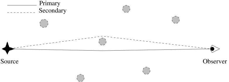
Figure 21: SIS universe.

10.3 One-lens approximation for point masses

Here, we will discuss reasonable corrections when images are non-separable. Since we have a very large number of images with two or more caustic crossings contributing to the flux of the total image, we can not correct for each one of them. Instead, we will make a first correction for the brightest secondary image using the approximation that lensing effects from a single lens (cell) is dominant. This is the so called one-lens approximation. Possible tests of the validity of this assumption is discussed in Sect. 11. Its plausibility is also reinforced by Figs. 8 and 9 in HW.

We can now use standard analytical expressions for one-lens systems for this correction:

$$\mu_{\rm corr}=|2\mu-1|.$$ (61)

In fact, this formula is valid also for secondary images but one then has to include the sign in $\mu$, i.e., $\mu_{2}<0$. However, Eq. (61) is only valid for the brightest secondary image, and one should therefore not apply it to very weak, secondary images. Also note, that to make the correction self-consistent, the magnification should be defined as the ratio of the expected area if the most prominent cell is empty and the real area. It is easy to see that the most important effect of this correction is to make the high magnification tail more pronounced.

10.4 One-lens approximation for SIS lenses

It is as straightforward to compute the total magnification using the one-lens approximation with a SIS-lens. For a primary image we get

$$\mu_{\rm corr}=2(\mu_{1}-1).$$ (62)

For a secondary image we get

$$\mu_{\rm corr}=2(1-\mu_{2}).$$ (63)

Since images are separable in the majority of cases, this is perhaps most interesting to use as a consistency check for the total luminosity.

11 Consistency checks

In order to validate our implementation of the method, we have performed a number of tests.

• Filled and empty beam distances
  First – in order to get an independent check – we have compared results from our implementation of the HW method using empty cells and cells with a homogeneous dust component with analytical empty-beam and filled-beam results (using the Angsiz routine, see Kayser et al. Kayser1995 (1995)). This has been done for a variety of cosmologies and the agreement is good even at very high $z$ (less than 1 % discrepancy up to $z=10$).

• Comparison with HW
  Second, we have reproduced most of the plots presented by HW. We have also tested that primary images satisfy $\frac{1}{N_{\rm tot}}\sum A_{1}\geq 1$, see Fig. 22.

  

  Figure 22: Sum of primary areas divided by $N_{\rm tot}$ for point masses (triangles) and NFW halos (crosses) in a $\Omega_{M}=0.3$, $\Omega_{\Lambda}=0.7$ universe. The number of primary images for each data point is $N_{1}=20\,000$.

• Average luminosities
  Imagine a source situated at the center of the sphere in the lower panel of Fig. 2 and observers sitting on the sphere at some constant redshift. Since the number of photons emitted by the source, as well as the area of the observers sphere is constant, i.e. independent of any details of the distribution of matter as long as the average matter density is the same, observers will on average receive the same flux, regardless of the matter distribution. This average will be equal to the FL value,

  $$\langle\mu\rangle=\mu_{\rm FL}.$$ (64)

  When computing $\mu$ for a source, one has to consider the total flux if there are multiple images. If we consider primary images only, without any corrections, we would expect to obtain a $\mu$ slightly lower than the FL value (since we lose some flux in secondary images).

  Note that this does not mean that the average area should equal the FL area. Instead,

  $$\langle\mu\rangle=\frac{1}{N}\sum_{i=1}^{N}\frac{A_{\rm empty}}{A_{i}} = \frac{A_{\rm empty}}{A_{\rm FL}}\Rightarrow$$

  $$\frac{1}{A_{\rm FL}} = \frac{1}{N}\sum_{i=1}^{N}\frac{1}{A_{i}},$$ (65)

  i.e., the FL area is the harmonic mean of the event areas, not the arithmetic (remember that $\langle A\rangle_{\rm Harm}<\langle A\rangle_{\rm Arit}$). Since we lose some flux in secondary images, we have (considering primary images only)

  $$A_{\rm FL}<\langle A\rangle_{\rm Harm}<\langle A\rangle_{\rm Arit}.$$ (66)

  See Fig. 23 for a plot of the average magnification using point mass lenses and NFW lenses. The result for SIS halos is not plotted since the result is indistinguishable from the NFW result. Note that since the deviation from the filled-beam value is due to the absence of the flux contained in secondary images, Fig. 23 indicates that the flux in secondary images is very low when using NFW or SIS halos, even at very high redshifts.

  

  Figure 23: Average magnification of primary images (normalized to filled-beam values) for point masses (triangles) and NFW halos (crosses) in an $\Omega_{M}=0.3$, $\Omega_{\Lambda}=0.7$ universe. The number of primary images for each data point is $N=20\,000$.

  The relationship between this test and the area test of HW is discussed in Appendix C.

12 Analytical fitting formulas

Since the numerical work involved in computing the results presented in this paper is quite extensive, it may be convenient to use simple analytical fitting formulas for the probability distributions for the different cosmologies, which we now give.

The probability distribution of the deviations from filled-beam magnitudes induced by SIS and NFW lenses, $\Delta=$mag(filled beam)$-$mag(lensed), can be parametrized by an exponential function folded with a gaussian distribution:

$$P(\Delta)\propto\int_{0}^{\infty}{e^{-\left(\Delta-\mu-m^{\prime}\right)^{2}\over 2\sigma^{2}}\cdot e^{-{\left(m^{\prime}\over\tau\right)}}dm^{\prime}}$$ (67)

Thus, for any combination of cosmological parameters, the corrections due to gravitational lensing can be described by three parameters: the mean of the gaussian distribution, $\mu$, the standard deviation $\sigma$, and the magnification tail, $\tau$. The expression in Eq. (67) can be rewritten so that (after normalization) a simpler integral is invoked:

$$P(\Delta)={1\over 2\sigma}e^{\left({\tau/\sigma-2(\Delta-\mu)\over 2\sigma}\right)}\cdot{\rm erfc}\left({\tau/\sigma-(\Delta-\mu)\over\sqrt{2\tau}}\right)$$ (68)

where

$${\rm erfc}(x)={2\over\sqrt{\pi}}\int_{x}^{\infty}{e^{-x^{\prime 2}}dx^{\prime}}$$ (69)

In Fig. 24 the fits to the magnification distributions are shown for SIS lenses for source locations $z=1$, $2$ and $3$ and for three different cosmologies. In Fig. 25 the same source locations and cosmologies are used but the lenses are of NFW type.

Figure 24: Fits of magnification distributions for SIS lenses using the analytical expression in Eq. (68).

Figure 25: Fits of magnification distributions for SIS lenses using the analytical expression in Eq. (68)

The parametrization of Eqs. (67) and (68) may be used to study the shape of the magnification distribution as a function of redshift and cosmological parameters, as shown in Figs. 26 and 27.

The estimates of the cosmological parameters may be further refined and the understanding of the mass distribution in galaxy halos could be deduced by fitting the parameters $\tau$, $\sigma$ and $\mu$ to the residual magnitude distributions in future high-redshift supernova searches, such as the SNAPsat project or at NGST. The accuracy of this method will be discussed in a forthcoming paper (Bergström et al., in preparation).

Figure 26: Redshift and cosmology dependence of parameters in Eqs. (67) and (68) for SIS lenses.

Figure 27: Redshift and cosmology dependence of parameters in Eqs. (67) and (68) for NFW lenses.

13 Discussion

In this paper, the method of Holz & Wald (art:HolzWald1998 (1998)) has been generalized to include the effect of non-vanishing pressure. A motivation for this exercise is to use this method as part of a large package for a detailed simulation of most aspects high-redshift supernova determination of the geometry of the universe (Bergström et al., in preparation). The possibility to allow for various matter contributions is then desirable. Another improvement has been to allow for a more realistic mass profile of the galaxy halos, the Navarro-Frenk-White distribution, where we have given analytical formulas for the geodesic deviation integrals. With this improvement, and by adding matter in our model universes according to a Schechter function with parameters fixed by observation, we think we have achieved a sufficient degree of sophistication to make realistic predictions of the lensing effects of present and future deep supernova searches.

Our results show, in agreement with previous work (Holz & Wald art:HolzWald1998 (1998); Metcalf & Silk metcalf (1999)) that the (unlikely) case of having most of the dark matter distributed in the form of point masses can be quite easily distinguished from more realistic halo models, if a sufficient number of supernovae can be detected at large redshifts. It will be more difficult to distinguish between a singular isothermal sphere model and the N-body results of Navarro, Frenk and White, unless $\Omega_{M}$ is large and one can measure supernovae out to $z\sim 2$ (see Fig. 12). However, this also means that our method of determining the properties of the lens population by matching the measured Schechter function with the required $\Omega_{M}$ gives quite robust results for the predicted magnifications of Type Ia supernovae over a broad range of reasonable halo models. This will be helpful when making realistic predictions for future deep supernova searches.

Appendix Appendix A : $J^{\alpha}\!_{\beta}$ for the Navarro-Frenk-White matter distribution

In this Appendix, we give analytic expressions for the integrals (28) needed for the evolution of the optical matrix for a bundle of light which passes near a mass distribution of the NFW form. We assume a spherically symmetric matter distribution, the impact parameter is $b$, the characteristic radius of the NFW model is $R_{s}$ and the cell radius is $R_{c}$. When $R_{s}\neq b$, it follows that

$$(J^{\rm NFW})^{X}\!_{X} = 2C\left\{\frac{\sqrt{R_{c}^{2}-b^{2}}(R_{s}^{2}-2R_{c}^{2}-b^{2})}{R_{c}^{2}(R_{s}+R_{c})(R_{s}^{2}-b^{2})}\right.$$ (70)

$$+\frac{2}{b^{2}}\ln\left[\frac{R_{c}}{b}+\sqrt{\left(\frac{R_{c}}{b}\right)^{2}-1}\right]$$

$$-\frac{\sqrt{R_{c}^{2}-b^{2}}(2R_{c}^{2}+b^{2})}{b^{2}R_{c}^{3}}\ln\left(1+\frac{R_{c}}{R_{s}}\right)$$

$$\left.+\frac{2R_{s}(R_{s}^{2}-2b^{2})}{b^{2}|R_{s}^{2}-b^{2}|^{3/2}}f(b,R_{s},R_{c})\right\},$$

$$(J^{\rm NFW})^{Y}\!_{Y} = -2C\left\{\frac{\sqrt{R_{c}^{2}-b^{2}}}{R_{c}^{2}(R_{s}+R_{c})}\right.$$ (71)

$$+\frac{2}{b^{2}}\ln\left[\frac{R_{c}}{b}+\sqrt{\left(\frac{R_{c}}{b}\right)^{2}-1}\right]$$

$$-\frac{\sqrt{R_{c}^{2}-b^{2}}(2R_{c}^{2}+b^{2})}{b^{2}R_{c}^{3}}\ln\left(1+\frac{R_{c}}{R_{s}}\right)$$

$$\left.+\frac{2R_{s}\,{\rm sgn}(R_{s}-b)}{b^{2}|R_{s}^{2}-b^{2}|^{1/2}}f(b,R_{s},R_{c})\right\},$$

$$(J^{\rm NFW})^{X}\!_{Y} = (J^{\rm NFW})^{Y}\!_{X}=0$$

$$f(b,R_{s},R_{c}) = \left\{\begin{array}[]{l}\!\!\ln\!\left(\!\frac{b^{2}+R_{s}R_{c}-\sqrt{R_{s}^{2}-b^{2}}\sqrt{R_{c}^{2}-b^{2}}}{b(R_{s}+R_{c})}\!\right)\,(R_{s}>b)\\ \arctan\left(\frac{\sqrt{b^{2}-R_{s}^{2}}\sqrt{R_{c}^{2}-b^{2}}}{b^{2}+R_{s}R_{c}}\right)\quad(R_{s}<b)\end{array}\right.,$$ (74)

and the limit $R_{s}\rightarrow b$ is:

$$(J^{\rm NFW})^{X}\!_{X} = 2C\left\{\frac{2}{b^{2}}\ln\left[\frac{R_{c}}{b}+\sqrt{\left(\frac{R_{c}}{b}\right)^{2}-1}\right]\right.$$

$$-\frac{\sqrt{R_{c}^{2}-b^{2}}(2R_{c}^{2}+b^{2})}{b^{2}R_{c}^{3}}\ln\left(1+\frac{R_{c}}{b}\right)-$$

$$\left.\left(\frac{R_{c}-b}{R_{c}+b}\right)^{3/2}\frac{R_{c}^{2}+3(R_{c}+b)^{2}}{3R_{c}^{2}b^{2}}\right\},$$

$$(J^{\rm NFW})^{Y}\!_{Y} = -2C\left\{\frac{\sqrt{R_{c}^{2}-b^{2}}}{R_{c}^{2}(R_{c}+b)}\right.$$ (75)

$$+\frac{2}{b^{2}}\ln\left[\frac{R_{c}}{b}+\sqrt{\left(\frac{R_{c}}{b}\right)^{2}-1}\right]$$

$$-\frac{\sqrt{R_{c}^{2}-b^{2}}(2R_{c}^{2}+b^{2})}{b^{2}R_{c}^{3}}\ln\left(1+\frac{R_{c}}{b}\right)$$

$$\left.-2\frac{\sqrt{R_{c}^{2}-b^{2}}}{b^{2}(R_{c}+b)}\right\}.$$

The constant $C$ is given by

$$C=\rho_{\rm crit}\delta_{c}R_{s}^{3}=\frac{M}{\ln(1+x_{c})-\frac{x_{c}}{1+x_{c}}},$$ (76)

where $x_{c}=R_{c}/R_{s}$.

Appendix Appendix B : Parameter values for mass distribution

Here, we have compiled various parameter values, relevant for the mass distribution discussed in Sect. 7. In what follows, absolute magnitudes are denoted by ${\cal M}$, while masses are denoted by $M$.

Lin et al.

See Eq. (32) of (Lin et al. lin (1996)).

• $\alpha=-0.70\pm 0.05$

• ${\cal M}_{*}-5\log h=-20.29\pm 0.02$

• $n_{*}=(1.9\pm 0.1)\cdot 10^{-2}\,h^{3}{\rm\ Mpc}^{-3}$

Lin et al. gives its range of validity as $-23.0\leq{\cal M}\leq-17.5$, which is about $\pm 2.7$ magnitudes around their characteristic magnitude $-20.29$. This translates into a luminosity range $L\in L_{*}10^{0.4\cdot 2.7}$, and a mass range $M\in M_{*}10^{0.4\cdot 2.7/(1-\beta)}$, which, with $\beta=0.2$, gives $M/M_{*}\in[0.045,22.4]$.

Kirshner et al.

(Kirshner et al. KI83 (1983); KI)

• $\alpha_{J}=-1.25$  (KI 19)
  $\alpha_{F}=-1.25$  (KI 22)

• ${\cal M}_{*,J}=-21.70$  (KI 18)
  ${\cal M}_{*,F}=-22.70$  (KI 21)

• $L_{*}=1.0\cdot 10^{10}h^{-2}L_{\odot}$ (see Binney & Tremaine BT87 (1987)).

• $n_{*}=1.2\cdot 10^{-2}h^{3}{\rm\ Mpc}^{-3}$  (KI 23)

Peebles

(Peebles book:Peebles (1993); PE)

• $\beta=0.2$  (PE 3.39)

• $\alpha=-1.07\pm 0.05$  (PE 5.130)

• ${\cal M}_{*}=-19.53\pm 0.25+5\log h$ in the $b_{J}$ magnitude system where ${\cal M}_{\odot}=5.48$.  (PE 5.139, 5.140)

• $L_{*}=1.0\cdot 10^{10}e^{\pm 0.23}h^{-2}L_{\odot}$  (PE 5.141)

• $n_{*}=1.0\cdot 10^{-2}e^{\pm 0.4}h^{3}{\rm\ Mpc}^{-3}$  (PE 5.142)

• $v_{*}=220\mbox{ km/s}$  (PE 3.35)

• $\lambda=0.25$  (PE 3.35)

In the numerical work in this paper, we have used

• $\beta=0.2$

• $\alpha=-0.7$

• $L_{{\rm min}}=0.5L_{*}$

• $L_{{\rm max}}=2.0L_{*}$

• $n_{*}=1.9\cdot 10^{-2}\,h^{3}{\rm\ Mpc}^{-3}$

• $v_{*}=220\mbox{ km/s}$

• $\lambda=0.25$

Appendix Appendix C : Mean area vs. luminosity

Holz and Wald (art:HolzWald1998 (1998)) use the fact that the area of the boundary of the past of an observer should be very nearly equal to the area of the past light cone in the underlying FL model. From this they deduce that adding up all areas – counting beams with an even number of caustics as positive and beams with an odd number as negative – one should very nearly obtain the FL result, i.e., $\langle A_{0}\rangle\simeq A_{\rm FL}$, where the zero-subscript denote unweighted quantities. Here we investigate whether this claim is consistent with the fact that the average magnification should be equal to the FL magnification.

Imagine that, without weighting, we get an area distribution $n_{0}(A)$, where we assume that lensing effects are weak enough to only give primary images. According to HW, we then have

$$\langle A_{0}\rangle=\frac{\int n_{0}(A)AdA}{\int n_{0}AdA}=A_{\rm FL}.$$ (77)

In our simulations, the area distribution will be a convolution of $n_{0}(A)$ and a probability distribution $p\,(A)$,

$$n(A)=n_{0}(A)p\,(A)=n_{0}(A)\frac{A}{A_{\rm empty}}.$$ (78)

Since we want the harmonic mean of areas to be equal to the FL value, we get

$$\frac{1}{\langle A\rangle} = \frac{\int^{A_{\rm empty}}n(A)/A\,dA}{\int^{A_{\rm empty}}n(A)\,dA}$$ (79)

$$= \frac{\int^{A_{\rm empty}}n_{0}(A)/A_{\rm empty}dA}{\int^{A_{\rm empty}}n_{0}(A)A/A_{\rm empty}dA}=\frac{1}{\langle A_{0}\rangle}.$$

That is, the two consistency checks at least show consistency in the case where we only have primary images. The inclusion of non-primary images is highly non-trivial since the concept of negative areas is difficult to interpret as luminosities. One possibility is to combine this approach with the one-lens approximation method for multiple image correcting. However, this is difficult to do analytically since one would then need the form of $n_{0}(A)$.

References

- (1) Battye R.A., Bucher M., Spergel D.N., 1999, preprint astro-ph/9908047
- (2) Bergström L., Goobar A., 1999, Cosmology and Particle Astrophysics (Wiley/Praxis, Chichester)
- (3) Binney J., Tremaine S., 1987, Galactic Dynamics, (Princeton University Press, Princeton)
- (4) Bullock J.S., et al., 1999, preprint astro-ph/9908159
- (5) Dahlén T., Fransson C., 1999, A&A 350, 349
- (6) Del Popolo A., 1999, preprint astro-ph/9908195
- (7) Ehlers J., Schneider P., 1986, A&A 168, 57
- (8) Falco E.E., Kochanek C.S., Munoz J.A., 1998, ApJ 494, 47
- (9) Garnavich P.M., et al., 1998, ApJ 493, 53
- (10) Goliath M., Ellis G.F.R., 1999, Phys. Rev. D 60, 023502
- (11) Goobar A., Perlmutter S., 1995, ApJ 450, 14
- (12) Hawking S.W., Ellis G.F.R., 1973, Large-scale structure of space-time (Cambridge University Press, Cambridge)
- (13) Holz D.E., Wald R.M., 1998, Phys. Rev. D 58, 063501
- (14) Jain B., Seljak U., White S., 1999, preprint astro-ph/9901191
- (15) Kayser R., Helbig P., Schramm T., 1995, A&A 318, 680
- (16) Kirshner R.P., et al., 1983, AJ 88, 1285
- (17) Lin H., et al., 1996, ApJ 464, 60
- (18) Metcalf R.B., Silk J., 1999, ApJ 519, L1
- (19) Miralda-Escudé J., Rees M.J., 1997, ApJ 478, L57
- (20) Navarro J.F., Frenk C.S., White S.D.M., 1997, ApJ 490, 493
- (21) Peebles P.J.E., 1993, Principles of physical cosmology (Princeton University Press, Princeton)
- (22) Perlmutter S., et al., 1999, ApJ 517, 565
- (23) Porciani C., Madau P., preprint astro-ph/9810403 (to appear in ApJ)
- (24) Premadi P., Martel H., Matzner R., 1998, ApJ 493, 10
- (25) Riess A.G., et al., 1998, AJ 116, 1009
- (26) Schneider P., Ehlers J., Falco E.E., 1992, Gravitational Lenses (Springer-Verlag, Berlin)
- (27) Turner E. L., 1990, ApJ 365, L43
- (28) Wald R. M., 1984, General Relativity (University of Chicago Press, Chicago)
- (29) Wambsganss J., Cen R., Ostriker J.P., 1998, ApJ 494, 29
- (30) Wang L., Caldwell R.R., Ostriker J.P., Steinhardt P.J., 1999, preprint astro-ph/9901388