A New Strategy for Deep Wide-Field High Resolution Optical Imaging.

Abstract

We propose a new strategy for obtaining enhanced resolution (FWHM $\simeq 0^{\prime\prime}.12$) deep optical images over a wide field of view. As is well known, this type of image quality can be obtained in principle simply by fast guiding on a small ($D\sim 1.5$m) telescope at a good site, but only for target objects which lie within a limited angular distance of a suitably bright guide star. For high altitude turbulence this ‘isokinetic angle’ is approximately $1^{\prime}$. With a 1 degree field say one would need to track and correct the motions of thousands of isokinetic patches, yet there are typically too few sufficiently bright guide stars to provide the necessary guiding information. Our proposed solution to these problems has two novel features. The first is to use orthogonal transfer charge-coupled device (OTCCD) technology to effectively implement a wide field ‘rubber focal plane’ detector composed of an array of cells which can be guided independently. The second is to combine measured motions of a set of guide stars made with an array of telescopes to provide the extra information needed to fully determine the deflection field. We discuss the performance, feasibility and design constraints on a system which would provide the collecting area equivalent to a single $9$m telescope, a 1 degree square field and $\simeq 0^{\prime\prime}.12$ FWHM image quality.

1 Introduction

Imaging surveys are limited by depth, angular coverage and angular resolution. There are currently several proposals for wide field telescopes and instrumentation which promise great gains in the first two of these variables (the CFHT MegaPrime Project ([Boulade et al. 1998]; [CFHT MegaPrime Project Web Site 1999]); Megacam on the MMT ([Conroy et al. 1998]; [McLeod et al. 1998]; [Geary & Amato 1998]; [MMT Megacam Project Web Site 1999]); the UK ‘Vista’ project [Vista Web Site 1999]; the ‘Dark Matter Telescope’ [Dark Matter Telescope Web Site 1999]; Suprime-Cam for Subaru [Subaru Suprime-Cam Web Site 1999]; Omega-Cam for the ESO VST at Paranal [OmegaCAM Web Site 1999]; the Canadian CFHT 8m upgrade proposal). Unfortunately, these designs are hampered by the limited angular resolution available from the ground; at $m\sim 25$ most faint galaxies are poorly resolved at even the best sites, and we know from e.g. the Hubble Deep Field that galaxies become still smaller as one pushes fainter, and there is a wealth of data lying tantalizingly beyond the resolution of conventional ground-based telescopes.

Atmospheric seeing arises from spatial fluctuations in the refractive index associated with turbulent mixing of air with inhomogeneous entropy and/or water vapor content (e.g [Roddier 1981]). High order adaptive optics (AO) can achieve spectacular improvement in angular resolution on large telescopes (see e.g. the reviews of [Beckers 1993]; [Roddier 1999]), but has not been applied to wide-field imaging due to the limited ‘isoplanatic angle’ this being the angular distance around the guide star within which target objects sample effectively the same refractive index fluctuations. There have been discussions of ‘multi-conjugate’ systems to increase the field of view (e.g. ?)), but little concrete has yet to emerge from this. Here we shall explore the possibility of of achieving a more modest but still valuable gain in resolution by using an array of small telescopes with fast guiding or ‘tip-tilt’ correction. In what follows we will first review why one would want to use tit-tilt on small telescopes, we then discuss the ‘isoplanatic angle’ problem for fast-guiding, and how this can be overcome using multiple telescopes and new technology in the form of ‘orthogonal transfer’ CCD technology.

Fast guiding is a common feature of modern large telescope designs, and can be quite useful for dealing with ‘wind shake’ or other local sources of image wobble. However, for realistic turbulence spectra, and for most sensible measures of image quality, fast guiding has relatively little effect on the atmospheric contribution to seeing for large telescopes. For fully developed Kolmogorov turbulence (e.g. [Tatarski 1961]) the structure function for phase fluctuations is $S_{\varphi}(r)\equiv\langle(\varphi(r)-\varphi(0))^{2}\rangle=6.88(r/r_{0})^{5/3}$. This says that the rms phase difference between two points grows in proportion to the $5/6$ power of their separation. The character of the phase fluctuations imposed on wavefronts is shown in figure 1. The amplitude of the phase fluctuations is characterized by the ‘Fried length’ $r_{0}$ [Fried 1965], which is the separation for which the rms phase difference is of order unity (actually $\sqrt{6.88}$ radians), and is on the order of 20cm at good sites in the visible).

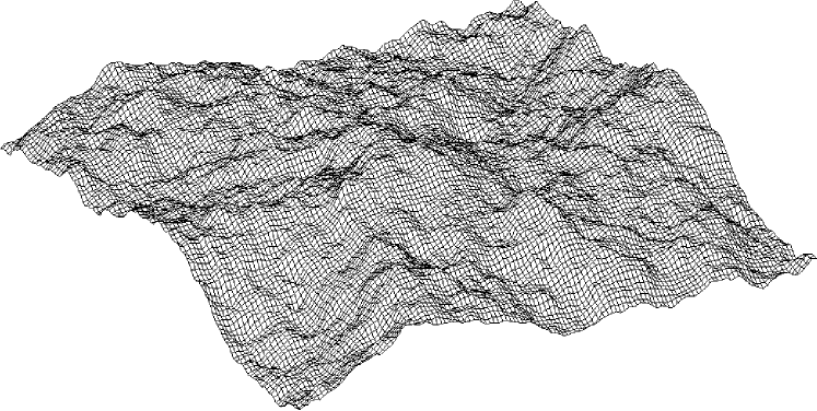
Figure 1: A realization of the phase fluctuation $\varphi({\bf r})$ produced by atmospheric turbulence with a $P(k)\propto k^{-11/3}$ Kolmogorov law power spectrum. This is the form of an initially flat wavefront from a distant source after it has propagated thought the atmosphere. No scales are shown for the axes because the power-law power spectrum gives rise to a ‘scale-invariant’ statistical topography; a blow-up of a region of this realization is, aside from a scaling of amplitude, statistically indistinguishable from the original,

The rapidly growing amplitude of the structure function means that the phase variations are dominated by the lowest order modes. For example, if we ignore piston, the phase variance averaged over a circular aperture of diameter $D$ is $\langle\varphi^{2}\rangle=1.013(D/r_{0})^{5/3}$ but this drops to $\langle\varphi^{2}\rangle=0.130(D/r_{0})^{5/3}$ if the lowest order Zernike modes of tip and tilt are removed [Fried 1965]. Thus applying tip-tilt correction reduces the phase variance by a factor $1.013/0.130=7.8$ which is both substantial and independent of the diameter of the telescope. We can safely conclude from this that a telescope with $D$ less than a few times $r_{0}$ will, after tip-tilt correction, have residual phase variance which is small compared to unity and will therefore give close to diffraction limited performance.

What about larger telescopes? If $D/r_{0}\gg$ a few then the residual phase variation is large compared to unity, so such telescopes will not be diffraction limited. As with a small telescope, the primary effect of tip-tilt is to reduce the phase fluctuations on scales of order the telescope diameter. This will cause a dramatic improvement in the transmission of the telescope for frequencies approaching the diffraction limit, but the uncorrected transmission for such frequencies is essentially zero, so even a large gain here does little good. There is some reduction in phase variations on smaller scales — separations on the order of $r_{0}$ that is — with some corresponding increase in useful image quality which we can estimate as follows: The root mean squared tilt of the wavefront averaged over the aperture is on the order of $\delta\theta\sim\delta\varphi\lambda/D\sim\sqrt{S_{\varphi}(D)}\lambda/D\sim\lambda/(D^{1/6}r_{0}^{5/6})$. More precisely, we find the variation in position the uncorrected PSF centroid to be a Gaussian $\exp(-\theta^{2}/2\sigma_{\rm tilt}^{2})$ with $\sigma_{\rm tilt}^{2}=0.169(\lambda/r_{0})^{2}(r_{0}/D)^{1/3}$ whereas the uncorrected PSF has FWHM $=1.0\lambda/r_{0}$ for $D\gg r_{0}$, which is the same as for a Gaussian with variance $\sigma_{\rm total}^{2}=0.181(\lambda/r_{0})^{2}$. To a crude approximation, which actually becomes quite good for $D\gg r_{0}$, one might expect the corrected PSF to approximate a Gaussian with $\sigma^{2}=\sigma_{\rm total}^{2}-\sigma_{\rm tilt}^{2}$ with corresponding improvement in image quality (which we take to be the inverse of the area of the PSF) of

$${\sigma_{\rm total}^{2}\over\sigma_{\rm total}^{2}-\sigma_{\rm tilt}^{2}}\simeq{1\over 1-0.93(D/r_{0})^{-1/3}}$$ (1)

so the gain from tip/tilt is predicted to decrease, albeit somewhat slowly, for large $D/r_{0}$. This theoretical expectation [Fried 1966] has been widely discussed and studied in detail ([Young 1974]; [Christou 1991]; [Glindemann 1997]; [Jenkins 1998]) and it turns out that, for a filled aperture, a pupil diameter $D\simeq 4r_{0}$ maximizes the normalized Strehl ratio, this being defined as the central value of the normalized PSF as compared to that for a large telescope, and the gain for $D=4r_{0}$ is a factor $\simeq 4.0$. For $D/r_{0}=10$ the gain is $\simeq 2.0$ and for $D/r_{0}=50$ the gain is a factor $1.4$. These latter numbers are in quite good agreement with the crude estimate (1). This expectation has also been confirmed in practice by ?) who used HRCAM on the CFHT with the pupil stopped down to $D=1.2$m, and by ?) with the UH adaptive optics system working in tip/tilt mode again with the CFHT stopped down to 1m aperture. These conclusions are somewhat dependent on the assumption of fully developed Kolmogorov turbulence. Recently ?) have reported deviations from the $P(k)\propto k^{-11/3}$ law at La Silla which they characterize, in the context of the von-Karman model, as an ‘outer-scale’ of $\sim 20$m, and a number of the measurements reviewed by ?), have also given fairly small values. A finite value for the outer scale will tend to further reduce the effect of tip-tilt correlation on large telescopes.

Another way to look at this problem is in terms of ‘speckles’. A snapshot of the PSF for a large telescope consists of a set of speckles, each of which is about the size of the diffraction limited PSF, and there being on the order of $N\sim D^{2}/r_{0}^{2}$ speckles in total, i.e. on the order of the number of $\sim r_{0}$ sized patches within the pupil. These speckles dance around on the focal plane (see http://www.ifa.hawaii.edu/$\sim$kaiser/wfhri for an animated movie showing the evolution of PSFs for a range of telescope diameters). For $D/r_{0}\simeq 4$ it is found that much of the time a substantial fraction of the light (say 25% or so) is in a single bright central speckle, and by tracking the centroid --- or better still tracking the peak of the brightest speckle [Christou 1991] --- one can keep this bright dominant speckle at a fixed point on the focal plane, resulting in a PSF with a diffraction limited core component.

For Kolmogorov turbulence the seeing angle (defined as the FWHM of the PSF) is $\Delta\theta=0^{\prime\prime}.5(\lambda/0.5\mu{\rm m})(r_{0}(\lambda)/20{\rm cm})^{-1}$ with $r_{0}(\lambda)\propto\lambda^{6/5}$. Analysis of SCIDAR measurements at Mauna Kea by ?) gave a median $\Delta\theta=0^{\prime\prime}.43$ at $\lambda=0.5\mu{\rm m}$ corresponding to $r_{0}(\lambda=0.5\mu{\rm m})=22.6$cm or, in the I-band, $r_{0}(\lambda=0.8\mu{\rm m})=40.0$cm for which the optimal telescope diameter is then $D=1.6$m. A similar value of the mean free atmosphere Fried length ($r_{0}=30$cm at $\lambda=0.55\mu{\rm m}$) was inferred by ?) from correlation of the modulation transfer function for wide binary stars of various separations. This would suggest a 20% larger optimal diameter, but the result is dependent on their assumed model for the vertical distribution of seeing. Racine also found an approximately log-normal distribution of seeing angle with 1-sigma points of $\Delta\theta=0^{\prime\prime}.29,\;0^{\prime\prime}.66$ corresponding to a range of $r_{0}(\lambda=0.5\mu{\rm m})=33.9,\;15.1$cm, and to a range in wavelength for which $r_{0}$ is optimally matched to a 1.6m telescope of $\lambda(r_{0}=40{\rm cm})=0.57,1.12\mu$m. Thus in the normal range of seeing conditions a $1.6$m diameter fast guiding telescope could operate optimally over the range of passbands V,R,I, Z. Note that in a multi-color survey performed in this way the resolution for the different passbands scales as FWHM $\propto\lambda$ rather than FWHM $\propto\lambda^{-1/5}$ as in a conventional survey.

Applying fast image-motion correction to a small telescope should therefore greatly enhance image quality, but only over a limited distance from the guide star used to measure the motion. Studies of the atmosphere using SCIDAR and thermosonde probes ([Barletti et al. 1976]; [Barletti et al. 1977]; [Roddier et al. 1990]; [Roddier et al. 1993]; [Ellerbroek et al. 1994]; [Racine 1996]; [Avila, Vernin, & Cuevas 1998]) have shown that the source of seeing (conventionally characterized by $C_{n}^{2}(h)$, the intensity of the power spectrum of refractive index fluctuations [Roddier 1981]) is highly structured and stratified. In the typical situation there is a substantial contribution from very low level turbulence --- the planetary boundary layer and ‘dome seeing’ --- but there are also comparable contributions from higher altitude layers at $h\sim 1-10$km. The indications are that the layers are thin with thickness on the order of 100m or so. The low level turbulence causes a coherent motion of all objects in the field, and is relatively easy to deal with. The higher altitude seeing is more problematic, since the angular scale over which images move coherently --- the ‘isokinetic’ angle --- is on the order of $D/h$. For $h=5$km say and $D=1.5$m this is roughly 1 arc-minute. It is perhaps worth mentioning at this point that the ?) experiment seemed to show a substantially larger isokinetic scale than the simple estimate given here. This is encouraging, as it would indicate a predominance of low-level turbulence, which would make our job easier, but it may well be that they were lucky and observed at a time when the high altitude seeing contribution was relatively quiescent.

The limited isokinetic angle has serious implications for wide field imaging. For a 1-degree field say, the focal plane will consist of $\sim 3000$ isokinetic patches moving independently, so one needs some kind of ‘rubber focal plane’ detector to track these motions. Moreover, at high galactic latitudes at least, the mean separation of stars which are sufficiently bright to guide on ($m\sim 16$) is on the order of $4^{\prime}$, so there are two few guide stars with which to determine the deflection field at all points on the focal plane.

One way to avoid the latter problem would be to work at lower galactic latitude, where bright guide stars are more abundant, or to peer through globular clusters, but these approaches seem rather unsatisfactory. The solution to these problems that we propose here has two key features. The first is to use OTCCD [Tonry, Burke, & Schechter 1997] technology to implement the rubber focal plane. The second is to use an array of telescopes to provide multiple samples of the atmospheric turbulence to provide the information needed to accurately guide out image motion at all points in the field of view.

In an OTCCD device, as in an ordinary CCD, the electrons created by impinging photons are are trapped in a grid of potential wells. The difference is that the origin of the grid can be shifted with respect to the physical pixels by fractional pixel displacements, and the accumulating charge can therefore be moved around quasi-continuously, and in multiple directions, to accommodate drifting of the images due to the atmosphere. A camera made of a large number of such devices could then shift charge on different parts of the focal plane independently.

To see how an array of telescopes might solve the problem of limited guide stars consider the simple case of a single thin layer of high-altitude turbulence at height $h$ above the telescope. A single small telescope monitoring a set of guide stars will provide a set of samples of the the image deflection field, scattered over a region of size $\sim h\Theta$ where $\Theta$ is the angular field size, but with spacing somewhat larger than the deflection coherence scale. A neighboring telescope observing the same set of stars will provide another set of samples of the deflection field with the same pattern as the first, but displaced by the vector separation of the telescopes as illustrated in figure 2. With an array of telescopes one can further increase the density of sampling of the deflection field until one has full coverage. In this scheme then, the information needed to guide out the motion of a target object image seen through some patch of the turbulent layer by a particular telescope would be provided by one or more other telescopes in the array which are viewing bright guide stars through the same patch of turbulence.

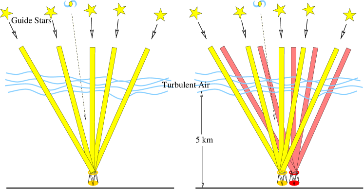
Figure 2: This figure shows schematically how an array of telescopes can be used to obtain effectively complete sampling of a high-altitude turbulent layer.

A single thin layer of turbulence is something of an idealization, and with multiple or thick layers one clearly needs more information. However, there is much more information at our disposal: a generic feature of Kolmogorov turbulence is that the turnover time for small scale eddies is long as compared to the time-scale for winds to convect the eddies through their length, so to some approximation we can adopt the ‘frozen turbulence’ assumption and use the additional information from positions of guide stars viewed at earlier times at points upwind of the point in question to constrain the deflection field.

Consider then an array of perhaps a few tens of small telescopes each acting as an incoherent detector --- there being no attempt here to co-phase the signals from separate telescopes as is done with a interferometer array --- but sharing the image motion data needed to implement low order AO in the form of fast guiding. Such an array, monitoring of order several hundred guide stars (for a nominal 1-degree field say) would provide many thousands of skewer like samples through the layers of turbulence flowing over the array. How though is one to make sense of this huge torrent of data in practice? We believe the answer is to exploit the statistically Gaussian nature of the turbulent layers. The eddy size which dominates the deflection here is on the order of the telescope diameter $D$. Assuming that the thickness of the turbulent layer exceeds this then the central limit theorem effectively guarantees that the phase perturbation $\varphi$ imposed on a wavefront passing through such a layer should be a statistically homogeneous and isotropic (though flowing) Gaussian random field. For fully developed Kolmogorov turbulence the power spectrum is $P_{\varphi}(k)\propto k^{-11/3}$ though this may flatten at low wave-number to something like the von Karman form $P(k)\propto(k^{2}+k_{0}^{2})^{-11/6}$ parameterized by $k_{0}\equiv 2\pi/\lambda_{0}$. In reality, atmospheric turbulence is intermittent, with the strength of the turbulence varying on time-scales of tens of minutes [Racine 1996], and this will break the very large-scale spatial homogeneity, but the process may well be effectively stationary on smaller length scales.

The deflection of the image centroid $\delta{\vec{\theta}}$ is, as we shall see below, obtained by taking the derivative of the phase perturbation and averaging over the telescope pupil. This is a linear function of the phase fluctuation field and so should also have Gaussian statistics, so this allows one to write down the joint probability distribution for a set of $N$ deflections $\delta\theta_{I}$ where $I$ is a compound index specifying the object, the telescope, the time of observation, and also the Cartesian component of the deflection:

$$p(\delta\theta_{0},\delta\theta_{1},\ldots)d^{N}\delta\theta={1\over\sqrt{(2\pi)^{N}|M|}}\exp(-\delta\theta_{I}M_{IJ}^{-1}\delta\theta_{J}/2)$$ (2)

where the covariance matrix is

$$M_{IJ}\equiv\langle\delta\theta_{I}\delta\theta_{J}\rangle.$$ (3)

This covariance matrix is a smooth and well defined function of the vector separation of the telescopes $\Delta{\bf x}$; the vector angular separation of the objects $\Delta\mbox{\boldmath$\theta$}$; and the time difference $\Delta t$. For sufficiently large fields one can obtain sufficiently dense sampling in $\Delta\mbox{\boldmath$\theta$}$ and by integrating over several minutes, it should be possible to accurately determine the deflection covariance function $\xi_{ij}(\Delta{\bf x},\Delta\mbox{\boldmath$\theta$},\Delta t)=\langle\delta\theta_{i}\delta\theta_{j}^{\prime}\rangle$. From this covariance matrix one can then compute the conditional probability for the deflection of a target object viewed with a given telescope at the current instant of time $t_{0}$ given the measured deflections of a set of guide stars for $t<t_{0}$. From this conditional probability $p(\delta\mbox{\boldmath$\theta$}_{\rm target}|\{\delta\mbox{\boldmath$\theta$}\}_{\rm guide\;stars})$ one can extract both the mean conditional deflection $\overline{\delta\mbox{\boldmath$\theta$}}$ --- which is the signal one uses to guide out the target object motion --- and also the covariance matrix for the errors in the guide signal $\sigma_{ij}=\langle(\delta\theta_{i}-\overline{\delta\theta_{i}})(\delta\theta_{j}-\overline{\delta\theta_{j}})\rangle$ which, as we shall see, allows one to compute the final PSF and thus monitor the performance of the system.

To summarize, the concept which emerges is of an array of telescopes, each equipped with its own wide field detector divided into a large number of segments, each of which is either continuously monitoring the position of a guide star or integrating. The guide star data is fed to a multi-variate Gaussian ‘probability engine’, which feeds back to the telescopes the necessary information for moving the accumulated charge on each integrating segment of the detector. As we shall see, under good conditions, such an instrument should allow $\simeq 0^{\prime\prime}.12$ FWHM image quality over large fields; while only a modest --- roughly a factor 3 --- increase in resolution over conventional telescopes we believe that this is well worth having as much of the information of interest in faint galaxy studies lies at spatial frequencies tantalizingly close to, but beyond the resolution attainable with a large aperture single mirror telescope. A nice feature of this design is that it scalable to arbitrarily large collecting area with cost proportional to area.

In the rest of this paper we will discuss in more detail the practicality of this approach. In §2 we present calculations of the PSF and optical transfer function (OTF) for fast guiding. We present a number of objective measures of the image quality which are relevant for different types of observation. We discuss the constraint on pixel size and telescope design imposed by the requirement that the image quality not be degraded by detector resolution. We also quantify how the PSF degrades with distance from the guide star. In §3 we consider the constraints imposed by the limited numbers of sufficiently bright guide stars. In §4 we discuss the spatial and temporal correlations of image motions. We outline our guiding algorithm and what constraints are imposed on the telescope array geometry. We find that there are currently insufficient data on the detailed structure and statistics of atmospheric turbulence to definitively determine the performance and optimize the design for the type of system we have in mind, but we describe the kinds of experiments that should be done to resolve this. In §5 we discuss the OTCCD ‘rubber focal plane’ detector. We consider the costs of software development in §6, and summarize the overall system cost in §7. In §8 we outline some of the scientific opportunities that this kind of instrument makes possible.

2 Image Quality with Fast Guiding

According to elementary diffraction theory (e.g. [Born & Wolf 1964]), the electric field amplitude at some position ${\bf x}_{\rm phys}$ on the focal plane of a telescope is the Fourier transform of the product of the telescope pupil function $T({\bf r})$ with the atmospheric phase factor $e^{i\varphi({\bf r})}$, so $E({\bf x}_{\rm phys})\propto\int d^{2}r\;T({\bf r})e^{i\varphi({\bf r})}e^{2\pi i{\bf x}_{\rm phys}\cdot{\bf r}/L\lambda}$. Here $L$ is the focal length and $\lambda$ is the wavelength. Squaring this gives the intensity which, suitably normalized, is the PSF $g({\bf x}_{\rm phys})$. In what follows it is convenient to work in rescaled focal plane coordinates ${\bf x}\equiv 2\pi{\bf x}_{\rm phys}/L\lambda$. The PSF is then the inverse Fourier transform of the OTF

$$g({\bf x})=\int{d^{2}z\over(2\pi)^{2}}\;e^{-i{\bf x}\cdot{\bf z}}\tilde{g}({\bf z})$$ (4)

where

$$\tilde{g}({\bf z})=\int d^{2}r\;T({\bf r})T({\bf r}+{\bf z})e^{i[\varphi({\bf r})-\varphi({\bf r}+{\bf z})]}$$ (5)

where we have normalized the pupil function so that $\int d^{2}r\;T^{2}({\bf r})=1$. These results are valid in the ‘near-field’ limit, which should be quite accurate for our purposes [Roddier & Roddier 1986].

In an idealized fast guiding telescope, the instantaneous PSF is measured from a bright ‘guide star’, and its position is determined and used to guide the telescope. In this section our goal is to determine the final corrected PSF averaged over a long integration time. Since the statistical properties of the phase fluctuation field $\varphi({\bf r})$ are given by Kolmogorov theory this is a well posed problem. It is however somewhat complicated, and the details of the PSF depend on the method used to determine the center. We first review the calculation of the ‘natural’ or uncorrected PSF in §2.1. We discuss the approximation to the corrected OTF given by [Fried 1966] in §2.2. In §2.3 we compute the OTF and PSF for the case of guiding on the image centroid. In §2.4 we show how the PSF for centroid guiding depends on the distance from the guide star. In §2.5 we discuss alternatives to the image centroid such as peak tracking, which yield somewhat superior image quality. Finally, in §2.6 we consider the effect of finite pixel size.

2.1 The Natural PSF

The long-exposure uncorrected OTF was first given in the classic paper of ?) and is obtained by taking the time average of (5). This requires the average of the complex exponential of the phase difference $\psi({\bf r},{\bf z})=\varphi({\bf r})-\varphi({\bf r}+{\bf z})$. At fixed ${\bf r},{\bf z}$ this is a stationary (in time) Gaussian random process with with probability distribution $p(\psi)=(2\pi\langle\psi^{2}\rangle)^{-1/2}\exp(-\psi^{2}/2\langle\psi^{2}\rangle)$ and so the time average of the complex exponential is

$$\langle e^{i\psi}\rangle=\int d\psi\;p(\psi)e^{i\psi}=\exp(-\langle\psi^{2}\rangle/2).$$ (6)

where the final equality follows on integrating by completing the square. Now since the phase fluctuation field is also a statistically spatially homogeneous process, the phase difference variance or ‘structure function’ $\langle\psi^{2}\rangle=\langle(\varphi({\bf r})-\varphi({\bf r}+{\bf z}))^{2}\rangle$ is a function only of the separation of the points: $\langle\psi({\bf r},{\bf z})^{2}\rangle=S(z)$, and so in this special case the OTF factorizes into the product of the diffraction limited OTF $\tilde{g}_{\rm diff}({\bf z})=\int d^{2}r\;T({\bf r})T({\bf r}+{\bf z})$ and the ‘atmospheric transfer function’ $\tilde{g}_{\rm atmo}(z)=\exp(-S(z)/2)$. For fully developed Kolmogorov turbulence the structure function is a power law $S(z)\propto z^{5/3}$ and the OTF therefore has the form $\tilde{g}(z)\propto\exp(-\alpha z^{5/3})$.

2.2 The Fried Model

A large part of the width of the natural PSF can be attributed to ‘wandering’ of the instantaneous PSF. This is illustrated in figure 3 which shows a set of realizations of the instantaneous PSF for a telescope with $D/r_{0}=4$. A series of animated images showing the continuous evolution of atmosphere limited PSFs can be viewed at http://www.ifa.hawaii.edu/$\sim$kaiser/wfhri. Fried argued that the corrected or ‘short-exposure’ OTF, i.e. that obtained after taking out any net shift in these instantaneous images before temporal averaging, should be of the form

$$\tilde{g}_{c}(z)\propto\exp(-\alpha z^{5/3}+\beta z^{2}).$$ (7)

This result has a very simple and intuitively reasonable physical interpretation: think of the uncorrected PSF as the convolution of the short exposure PSF with the distribution $p(\overline{{\bf x}})$ of the image shifts caused by any net tilt to the incoming wavefronts. For steady turbulence this distribution is a Gaussian, so in Fourier space its transform is also a Gaussian, and so the short exposure OTF should be the long-exposure form divided by a Gaussian which, for suitably chosen $\alpha$, $\beta$, is exactly what equation (7) states. The flaw in this argument --- as acknowledged by Fried in a footnote --- is that it assumes that the image shift is statistically independent of the other components of the wavefront distortion, which is not strictly correct (though for some purposes it is a pretty good model). Another limitation of Fried’s analysis is that it identifies the image shift with the tip and tilt Zernike coefficients of the wavefront. While this is qualitatively correct, the shift of the centroid of the image --- which is the quantity most readily measured in the type of system considered here --- differs somewhat from the tip/tilt coefficients. This problem has been reconsidered by several authors ([Young 1974]; [Christou 1991]; [Glindemann 1997]; [Jenkins 1998]) using a variety of approximations and/or simulation techniques. We now present a simple analytic calculation of the OTF and PSF for fast centroid guiding.

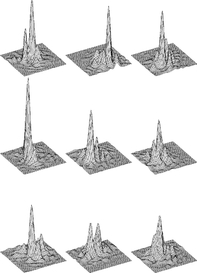
Figure 3: Numerical realizations of some instantaneous PSFs for a telescope with $D/r_{0}=4$ generated as described in §2.5. The box size here is $1^{\prime\prime}.2(\lambda/0.8\mu{\rm m})$, and the surfaces are normalized such that $\int d^{2}x\;g(x)=1$. These show graphically how the small telescope PSF typically contains a very sharp spike, which is effectively diffraction limited, but that this spike undergoes large random displacements.

2.3 PSF for Centroid Guiding

The photon weighted centroid is defined as

$$\overline{\bf x}\equiv\int d^{2}x\;{\bf x}g({\bf x}).$$ (8)

Now since $\tilde{g}({\bf z})=\int d^{2}x\;g({\bf x})e^{i{\bf k}\cdot{\bf z}}$, the gradient of the instantaneous OTF is $\nabla\tilde{g}({\bf z})=i\int d^{2}x\;{\bf x}g(x)e^{i{\bf x}\cdot{\bf z}}$, so the instantaneous centroid is given by the gradient of the OTF at the origin:

$$\overline{\bf x}=-i\nabla\tilde{g}(0)=-\int d^{2}r\;T^{2}({\bf r})\nabla\varphi({\bf r})=\int d^{2}r\;{\bf W}({\bf r})\varphi({\bf r})$$ (9)

where the second equality is obtained by direct differentiation of (5), and the final result follows on integrating by parts and defining the vector valued function ${\bf W}({\bf r})\equiv\nabla T^{2}({\bf r})$. The centroid is the average of the wavefront slope weighted by $T^{2}$ [Glindemann 1997]; the so-called ‘G-tilt’. Note that this is not quite the same as the ‘Z-tilt’ defined as the tip/tilt components of the Zernike decomposition of the wavefront; for a simple filled disk pupil function the Z-tilt coefficients are the integral of $T^{2}({\bf r}){\bf r}$ times $\varphi({\bf r})$ whereas in (9) the function ${\bf W}({\bf r})$ is non-zero only at the pupil edge. For low spatial frequency phase fluctuations the wavefront tip-tilt coefficients and the centroid are effectively identical, but they couple to high spatial frequency fluctuations rather differently. A key feature of the centroid is that it is a linear function of the random phase fluctuation field, a fact which greatly facilitates the following calculation.

We shall need the covariance matrix for the centroid deflections, which, from (9), is

$$\sigma_{ij}\equiv\langle{\overline{x}}_{i}{\overline{x}}_{j}\rangle=\int d^{2}r\int d^{2}r^{\prime}\;W_{i}({\bf r})W_{j}({\bf r})\langle\varphi({\bf r})\varphi({\bf r}^{\prime})\rangle$$ (10)

and the trace of which gives the variance of the centroid. For atmospheric turbulence $\varphi({\bf r})$ is a statistically isotropic and homogeneous random field so $\langle\varphi({\bf r}^{\prime})\varphi({\bf r})\rangle=\xi({\bf r}^{\prime}-{\bf r})$ where $\xi({\bf r})$ is the two-point function of the phase, and depends only on $|{\bf r}|$. For Kolmogorov turbulence the phase two-point function is formally ill-defined (in reality its value depends on the outer-scale cut-off) and it is more convenient to work with the phase structure function $S(r)\equiv\langle(\varphi({\bf r}^{\prime})-\varphi({\bf r}^{\prime}+{\bf r}))^{2}\rangle=2(\xi(0)-\xi(r))$ which is well defined and has a power-law form $S(r)=6.88(r/r_{0})^{5/3}$, where $r_{0}$ is the Fried length. To evaluate (10) then we replace $\langle\varphi({\bf r})\varphi({\bf r}^{\prime})\rangle$ by $\xi({\bf r}-{\bf r}^{\prime})=\xi(0)-S({\bf r}-{\bf r}^{\prime})/2$. The dependence on the cut-off dependent but constant term $\xi(0)$ drops out, and in terms of the structure function $S(r)$ the centroid covariance matrix is then

$$\sigma_{ij}=-{1\over 2}\int d^{2}r\;W_{i}({\bf r})(W_{j}\otimes S)_{{\bf r}}$$ (11)

where we have defined the convolution operator $\otimes$ such that $a\otimes b\equiv\int d^{2}r^{\prime}\;a({\bf r}^{\prime})b({\bf r}-{\bf r}^{\prime})$. The centroid covariance matrix has dimensions of $1/L^{2}$. For Kolmogorov turbulence

$$\sigma_{ij}=\alpha_{ij}D^{-1/3}r_{0}^{-5/3}$$ (12)

where $\alpha_{ij}$ is a dimensionless matrix depending only on the shape of the telescope input pupil. For a circularly symmetric pupil this matrix is diagonal and for a filled circular aperture we find, from numerical integration, that

$$\sigma_{ij}=6.68\delta_{ij}(D/r_{0})^{-1/3}r_{0}^{-2}.$$ (13)

The instantaneous centroid corrected PSF is, from (5),

$$g_{\rm c}({\bf x})=g({\bf x}+\overline{{\bf x}})=\int{d^{2}z\over(2\pi)^{2}}\;e^{-i{\bf x}\cdot{\bf z}}e^{-i{\bf z}\cdot\int d^{2}r^{\prime}\;{\bf W}({\bf r}^{\prime})\varphi({\bf r}^{\prime})}\int d^{2}r\;T({\bf r})T({\bf r}+{\bf z})e^{i[\varphi({\bf r})-\varphi({\bf r}+{\bf z})]}$$ (14)

so the average centroid corrected OTF for a long exposure, which we shall denote by $\tilde{g}_{c}({\bf z})$, can be written as

$$\tilde{g}_{\rm c}({\bf z})=\int d^{2}r\;T({\bf r})T({\bf r}+{\bf z})\langle e^{i\psi({\bf r},{\bf z})}\rangle$$ (15)

where

$$\psi({\bf r},{\bf z})\equiv\varphi({\bf r})-\varphi({\bf r}+{\bf z})-{\bf z}\cdot\int d^{2}r^{\prime}\;{\bf W}({\bf r}^{\prime})\varphi({\bf r}^{\prime})$$ (16)

Just as before, for given ${\bf r}$, ${\bf z}$, the phase factor $\psi({\bf r},{\bf z})$ is a stationary (in time) Gaussian random process so again $\langle e^{i\psi}\rangle=\exp(-\langle\psi^{2}\rangle/2)$ but where now

$$\matrix{\langle\psi({\bf r},{\bf z})^{2}\rangle=S({\bf z})-2{\bf z}\cdot\int d^{2}r^{\prime}\;{\bf W}(r^{\prime})[\langle\varphi({\bf r}^{\prime})\varphi({\bf r})\rangle-\langle\varphi({\bf r}^{\prime})\varphi({\bf r}+{\bf z})\rangle]+{\bf z}\cdot\mbox{\boldmath$\sigma$}\cdot{\bf z}\cr=S({\bf z})+{\bf z}\cdot[({\bf W}\otimes S)_{\bf r}-({\bf W}\otimes S)_{{\bf r}+{\bf z}}]+{\bf z}\cdot\mbox{\boldmath$\sigma$}\cdot{\bf z}}$$ (17)

and so the corrected OTF is

$$\tilde{g}_{c}({\bf z})=\int d^{2}r\;T({\bf r})T({\bf r}+{\bf z})e^{-[S({\bf z})+{\bf z}\cdot[({\bf W}\otimes S)_{\bf r}-({\bf W}\otimes S)_{{\bf r}+{\bf z}}]+{\bf z}\cdot\mbox{\boldmath$\sigma$}\cdot{\bf z}]/2}.$$ (18)

This equation, along with (11)and the definition ${\bf W}({\bf r})\equiv\nabla T^{2}$, allows one to compute the OTF $\tilde{g}_{\rm c}({\bf z})$ for a given spectrum of phase fluctuations $S(r)$ and pupil function $T({\bf r})$. For isotropic turbulence, and for a circularly symmetric input pupil, $g_{c}({\bf z})$ is only a function of $|{\bf z}|$, so one can take ${\bf z}$ to lie along the $x$-axis say in (18). Note that the terms involving ${\bf W}\otimes S$ in (18) are not independent of ${\bf r}$ and so one cannot factorize the fast guiding OTF into a product of $\tilde{g}_{\rm diff}$ and a purely atmospheric dependent term as was the case for the uncorrected OTF.

The ‘normalized Strehl ratio’ is shown in figure 4. This is the ratio of the central intensity of the normalized corrected PSF $g({\bf x}=0)=(2\pi)^{-2}\int d^{2}z\;\tilde{g}({\bf z})$ to that for a very large telescope, and is a useful measure of the image quality. This figure displays the well known result that according to this criterion the best image quality is obtained for telescope diameter $D\simeq 4r_{0}$; for smaller telescopes the seeing is limited by the size of the Airy disk while for larger telescopes tip/tilt or fast guiding becomes ineffective at reducing the phase variance.

Figure 4: The normalized Strehl ratio for fast centroid guiding is plotted as a function of $D/r_{0}$, the telescope diameter in units of the Fried length.

The point spread function $g({\bf x})$ computed as the Fourier transform of the OTF given by equation (18) is shown in figure 5 for fast guiding with a telescope of optimal diameter $D=4r_{0}$. Figure 6 shows the OTF and figure 7 shows the radial profile of the PSF. To set the physical scales in these examples the Fried length was taken to be $40$cm as appropriate for a good site like Mauna Kea at $\lambda\simeq 0.8\mu$m and which gives uncorrected FWHM $\simeq 0^{\prime\prime}.4$.

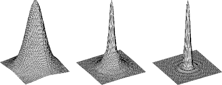
Figure 5: Left hand panel shows the PSF for natural seeing. The center panel shows the result of fast-guiding on a small telescope. The right hand panel shows the diffraction limited PSF. A wavelength $\lambda=0.8\mu$m, a Fried length of $40$cm and a telescope diameter of $D=1.6$m were assumed. The box side here is $1^{\prime\prime}.0$. The plots have been normalized to the same central value.

Figure 6: Optical transfer function for uncompensated (dashed) and centroid guided (solid) images. The dotted line is the Fried approximation. The dot-dot-dot-dash line is the OTF for a diffraction limited telescope.

Figure 7: PSF obtained by Fourier transforming the OTFs of figure 6. A wavelength $\lambda=0.8\mu$m, a Fried length of $40$cm and a telescope diameter of $D=1.6$m were used. The curves are normalized so that $\int d^{2}\theta\;g(\mbox{\boldmath$\theta$})=1$, except for the diffraction limited case which has been multiplied by $0.25$.

There is no unique way to characterize the image quality of a telescope. It is clear from figure 6 that the gain in signal (and therefore in signal to noise) is huge for frequencies approaching the diffraction limit of the telescope, where the natural seeing OTF is exponentially suppressed. Comparing the natural seeing and fast guiding PSFs we find:

• The normalized Strehl ratio is increased by a factor $4$.

• The FWHM is reduced by a factor $3.1$ from $0^{\prime\prime}.4$ to $0^{\prime\prime}.12$.

• The resolution, according to the Rayleigh-style measure of the separation of a pair of equally bright stars which just produce separate maxima after convolution, is improved by a factor $3.44$ from $0^{\prime\prime}.324$ to $0^{\prime\prime}.094$.

• The efficiency for detection of isolated point sources against a sky background, which is proportional to $\langle g\rangle\equiv\int d^{2}x\;g^{2}({\bf x})$, is increased by a factor $2.16$.

• The variance in position for a point source of flux $F$, detected as a peak of the image smoothed with the PSF, and seen on a noisy background with sky variance (per unit area) $\sigma^{2}$ is

  $$\langle\Delta x^{2}\rangle={8\sigma^{2}\int d^{2}x|\nabla g|^{2}\over F^{2}(\nabla^{2}g(x=0))^{2}}={8\sigma^{2}\over F^{2}}{\int{d^{2}z\over(2\pi)^{2}}z^{2}\tilde{g}^{2}(z)\over\left[{d^{2}z\over(2\pi)^{2}}z^{2}\tilde{g}(z)\right]^{2}}$$

  and is decreased by a factor $\sim 130$.

• The efficiency for weak-lensing measurements is also increased by up to about a factor 120 for small galaxies as we show in more detail in §8.1.

It is apparent that there is spectacular improvement in the quality of the core of the PSF. Crudely speaking, one can characterize the PSF as a near diffraction limited core, which, for $D/r_{0}=4$, contains about $1/4$ of the light, superposed on an extended halo with width similar to the uncorrected PSF. The low frequency ‘halo’ can be removed by spatial filtering, and images with effectively diffraction limited resolution can thereby be generated.

2.4 Isoplanatism

Equation (18) applies exactly only in the immediate vicinity of a guide star. What happens if we guide on the centroid of a certain star, but observe an object some finite angular distance $\Delta\mbox{\boldmath$\theta$}$ away? For a single deflecting screen at altitude $h$, equation (18) still holds, but with the understanding that $\bf W({\bf r})$ be displaced from the origin by $\Delta{\bf r}=h\Delta\mbox{\boldmath$\theta$}$. (It is also relatively straightforward to generalize the analysis here to allow for finite guide star sampling frequency, or to guide using some linear combination of centroids of a number of guide stars, but we shall not elaborate on that at this point). The result, for a range of distances from the guide star, is shown in figures 8, 9. It is interesting to note that if the range of the phase deflection correlations is limited to some correlation scale length $r_{c}$, as in the von Karman model for instance, so the structure function becomes flat at $r\gg r_{c}$, then the terms involving ${\bf W}\otimes S$ become negligible if we guide on a star which lies at distance far from the target object and we find the simple and intuitively reasonable result that the OTF is the product of the uncorrected OTF with $\exp(-{\bf z}\cdot\mbox{\boldmath$\sigma$}\cdot{\bf z}/2)$ or equivalently that the PSF is the convolution of the uncorrected PSF with $\exp(-{\bf x}\cdot\mbox{\boldmath$\sigma$}^{-1}\cdot{\bf x}/2)$ which is just the distribution of the centroid deflections $p({\bf x})$.

Figure 8: Contour plots of PSFs as a function of guide star distance. These were calculated for a single layer of turbulence, a telescope diameter $D=1.6$m, and are for target objects which sample the turbulent layer at distances 0, 0.25m, 0.5m, 1m, 2m, 4m, 8m from the guide star. These plots show the theoretically expected radial PSF anisotropy at intermediate separations.

Figure 9: Radially averaged profiles of PSFs as a function of guide star distance. These were calculated for a single layer of turbulence and are for target objects which sample the turbulent layer at distances 0, 0.25m, 0.5m, 1m, 2m, 4m, 8m from the guide star, just as in figure 8.

It is interesting to compare figure 8 with the results of [McClure et al. 1991]. They measured shapes of several stars up to $100^{\prime\prime}$ from the guide star and saw an increase in ellipticity with distance but very little increase in size. This suggests that their $100^{\prime\prime}$ separation corresponds to a physical separation of $\simeq 0.25-0.5$m and this would be consistent with a layer of turbulence at $h\simeq 1$km.

We have also compared the exact results obtained using (18) with the ‘Friedian’ approximation (that the uncorrected PSF is the convolution of the corrected PSF with $p({\bf x})$), which is

$$\tilde{g}_{\rm Fried}({\bf z})=e^{-{1\over 2}(S(z)-{\bf z}\cdot\mbox{\boldmath$\sigma$}\cdot{\bf z})}g_{\rm diff}({\bf z}).$$ (19)

We find that the approximate OTF agrees asymptotically with the exact calculation for small argument, but there are sizeable departures at large $z$, and consequently the high spatial frequency features of the PSF are not accurately reproduced.

2.5 Alternative Guiding Schemes

In the previous sections we considered in detail the case of guiding on the centroid. This was largely for the sake of mathematical convenience, as it allowed us to derive fairly simple but exact (at least in the near field limit) formulae for the PSF and OTF, but these may not be optimal. Alternatives to centroid guiding have been considered by ?), who has performed simulations to compare tip-tilt, centroid guiding and also the so called ‘shift and add’ or ‘peak tracking’ procedure where the image is centered on the peak of the brightest speckle. By construction, peak tracking will optimize the Strehl ratio. Other possibilities that will tend to give more weight to the central parts of the PSF, and which might therefore be expected to sharpen up the image quality near the peak, are to take the average of $x_{i}$, but weighted by some non-linear function of the PSF. For instance, one possibility would be to define the image center as

$$\overline{\bf x}=\int d^{2}x\;{\bf x}g^{2}({\bf x})/\int d^{2}x\;g^{2}({\bf x}).$$ (20)

To explore the performance of these alternative centering algorithms --- which are more difficult to treat analytically --- we have made simulations similar to those of Christou in which we generate a large number of realizations of Gaussian random field phase screens with Kolmogorov spectrum and compute the integrals (4), (5) numerically to obtain realizations of the speckly PSFs which we then re-center using various different algorithms and then sum the result. Some example PSFs were shown in figure 3. The result of averaging thousands of such PSFs with various re-centering schemes are shown in figures 10 and 11. The result of this analysis is that with the more sophisticated centering schemes considered here one can obtain a 15-25% improvement over centroid guiding and therefore an overall improvement in normalized Strehl ratio of about 5.

So far we have ignored the effect of read-noise and photon counting uncertainty in the guide star position determination. Of the schemes considered here these are most problematic for the centroid, and so noise considerations further favor peak tracking or some non-linear centroiding scheme. As we have seen, the photon weighted centroid is somewhat special in that it is a linear function of the atmospheric phase fluctuation, and as a consequence, should have accurately Gaussian statistical properties. For non-linear centroiding or peak tracking the deflection will not be strictly Gaussian --- the peak displacement will have discontinuities for instance --- but this does not seem to be a serious problem.

There is another subtle difference between peak tracking and centroiding which is how the evolutionary time-scale, and therefore the necessary sampling rate, depends on the height distribution of seeing. If the wind speed is $v$ then the time-scale for centroid motions is on the order of $\tau\sim D/v$, i.e. just the time it takes for the wind to cross the telescope pupil, regardless of whether the seeing arises in a single screen or in multiple layers. The speckle persistence time is also on the order $\tau\sim D/v$ for a single screen, but for multiple screens or a continuous distribution the persistence time is predicted to be $\tau\sim r_{0}/v$ [Roddier, Gilli, & Lund 1982]. This is rather worrying as it would suggest that one would need much faster temporal sampling than the single screen calculation suggests. However, from numerical realizations of evolving PSFS (see §3 below) we find this not to be the case; for $D/r_{0}\simeq 4$ we find that the timescale for peak motions is very similar for both single and multiple layer seeing, and that a sampling rate $\simeq 0.5-1D/v$ is adequate in either case.

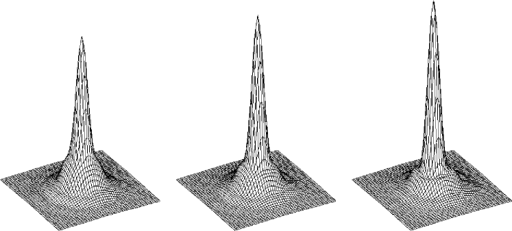
Figure 10: Surface plots of averaged PSFs computed numerically and re-centered using a variety of algorithms. On the left is the centroid. The center plot shows the result of centering on the $g^{2}$ weighted centroid as described in the text. On the right is shown the result for peak tracking. The PSFs are normalized to equal volume below the surface. The box size is $1^{\prime\prime}.0$.

Figure 11: Radial profiles of simulated PSFs as shown in figure 10. These show that the $g^{2}$ weighted centroid and peak tracking give further improvements in the Strehl ratio of $\sim 15\%$, $25\%$ respectively as compared to guiding on the centroid.

2.6 Pixelization Effects

In a regular CCD and with perfect guiding, the output image is a set of point like samples of the convolution of the true sky with a box-like pixel function. In an OTCCD device there is an additional degree of smoothing because the image moves continuously, yet the charge is shifted in discrete steps of finite size, so there is some fluctuation in image position about the effective pixel center which will have a box-like distribution function. In the design described in §5 below there are $\sim 10$ positions at which one can set the origin per physical pixel so this extra smoothing is relatively minor, corresponding to a 10% increase in the pixel area. To obtain a continuously sampled image it is necessary to combine a number of exposures. The image combination may involve interpolation and this will introduce some further smoothing of the image. The interpolation is however applied to the images after the photon counting noise is realized, so there is no information loss in this step, and the net effect of pixelization on signal to noise is the same as applying a single convolution with the pixel function.

This sets a constraint on the pixel angular scale if the pixelization is not to undo the improvement in image quality provided by guiding. To quantify this we have taken the exact fast guiding PSF and re-convolved with pixel functions of various sizes and measured the reduction in Strehl ratio. We find that a pixel size of $0^{\prime\prime}.1$ gives a reduction in Strehl of about 20%, which we feel is just acceptable. This sampling rate is about one half of the critical sampling rate for this combination of telescope diameter and wavelength.

2.7 Telescope Design Constraints

The main constraints on the design of the telescope are that it should have a primary mirror diameter of about $1.5$m and should be able to give diffraction limited images over a square field of side 1 degree or thereabouts. A further constraint is imposed by the cost of the detectors. Since their cost scales roughly as the area of silicon (rather than as the number of pixels) one would like to make the pixels as small as is practical. As we discuss below in §5 a pixel size of $5\mu$m seems reasonable.

In order to meet these requirements, we have explored several modified Ritchey-Chretien telescope designs employing a refractive aspheric corrector located near the focal plane. The designs give diffraction limited images over the required field of view, and we have concluded that these designs are readily buildable for a reasonable cost (see section 7).

We can also consider all-reflective systems to avoid diffraction spikes and scattered light from bright stars that may be a problem with refractive correctors. Such all reflective designs exist and we expect that they could be implemented for a comparable cost.

3 Guide Star Constraints

As discussed, in the Introduction, each telescope needs to measure positions of hundreds of guide stars scattered over the field. This is possible if the primary detector (a segmented OTCCD as described in more detail in §5) also serves as the guide star sensor. This has the advantage of avoiding the complication and expense of pick-off mirrors and auxiliary detector, and by fast read-out of a small patch around each guide star one can sample at rates in excess of 100 Hz which is more than adequate. Disadvantages of this approach are that one then loses that element of the CCD array, of say an arc-minute in size, for science, and that the guide stars must be observed through whatever filter is needed for the science measurements, with concurrent loss of photons. The purpose of this section is to provide estimates of the rate at which photons are collected as a function of telescope aperture and guide star brightness, the rate at which we must sample image motions, and the constraints these place on the number of usable guide stars.

Scaling from the performance of existing thinned CCD cameras on Mauna Kea, we expect that a good, backside illuminated CCD will accumulate about one electron per second from a source of $R$ magnitude

$$m_{1}=24.6+5\log(D/1.5\hbox{\rm m}),$$ (21)

(in the I-band the corresponding value is $24.3$). Hence an exposure of $\Delta t$ of a source of magnitude $m$ should yield $N$ electrons:

$$N=\Delta t\times 10^{-0.4(m-m_{1})}.$$ (22)

This is the total number of electrons. With fast guiding, what is more relevant is the number of electrons in the diffraction limited core of the PSF which is $N_{\rm core}=\alpha N$ with $\alpha\simeq 1/3$ for peak tracking.

The centroid or peak position will vary with time primarily because the deflecting screen is being convected along at the wind speed. In what follows we will adopt a fiducial speed of $15$m/s. This converts to a coherence time for peak motions of $\tau\sim D/v=0.1{\rm s}(D/1.5{\rm m})(v/15{\rm m/s})$. For given guide star brightness there is an optimal choice of sampling rate, since if the sampling rate is too high then the star centroid or peak location will be uncertain because of measurement error, while if the sampling rate is too slow the time averaged position will not accurately track the instantaneous position. To make this more quantitative we have made simulations in which we generated a large Kolmogorov spectrum phase screen from which extracted a sequence of closely spaced pupil-sized sub-samples, and for each of which we computed the instantaneous PSF using (5). This stream of PSFs was averaged in pixels with appropriate angular size according to subsection 2.6 above, and averaged in time with with some chosen integration time, and the result was then converted to a photon count by sampling in a Poissonian manner and adding read noise, the mean of which was taken to be $2e^{-}$. A simple peak-tracking algorithm --- locate the hottest pixel and then refine the position using 1st and 2nd derivative information computed from the neighboring pixels --- was then applied to the simulated pixellated images, and the PSF for target objects was calculated by shifting the instantaneous PSFs to track the peak and then averaging. This calculation was performed for a coarse grid of star luminosities and integration times. As expected, for bright objects we find the optimal sampling rate is quite high, while for fainter objects the measurement uncertainty tilts the balance towards longer integration times. A good compromise for realistic guide stars is to take an integration time of about $D/v$ corresponding to a sampling rate of about 10 Hz for our fiducial $15$m/s wind speed and diameter of $D=1.5$m. For very bright stars this is not optimal, but the gain obtained by sampling faster is rather small. With this sampling, we find negligible reduction in Strehl (as compared to rapid sampling of a very bright guide star) for stars which generate about 4000 electrons per second, or about 400$e^{-}$ per sample time, of which $\sim 140$ are in the diffraction limited core. This corresponds to an $R$ magnitude limit of

$$m_{4000}=15.6+7.5\log(D/1.5\hbox{\rm m})$$ (23)

($15.3$ in the I-band). The number of stars per square degree at the north galactic pole brighter than $R$ magnitude $m_{R}$ is approximately

$$\matrix{N({<}m_{R})=2.8\times 10^{-9}m^{9.2}\cr N({<}m_{I})=5.6\times 10^{-9}m^{9.1}}$$ (24)

Equation (24) is a good fit to the ?) model over the range $12<m<20$, and gives a number of sufficiently bright guide stars per square degree of approximately

$$N({<}m_{4000})=265\times(1+4.4\log(D/1.5\hbox{\rm m})$$ (25)

($340$ in the I-band).

This number density corresponds to a mean separation $\simeq 3^{\prime}.7$. As this is greater than the coherence angle for turbulence at altitudes higher than a few km, an instantaneous measurement of the deflections of a set of guide stars does not provide sufficient information to fully determine the deflection field. In making these estimates we have erred somewhat on the side of caution. For example, for stars which are a factor 4 ($\sim 1.5$ magnitudes) fainter than the limiting magnitude quoted above the resulting target image Strehl is reduced by about 30%, so there is still a reasonable fraction of light in the diffraction limited core (around $\sim 20$% rather than $\sim 30$% of the total) and this increased the number density of stars by about a factor 2.5. This result is illustrated in figure 12. Also, observations at lower galactic latitude will yield higher guide star densities by a factor ${\rm sec}(b)$, but the conclusion remains that over most of the sky the sampling provided by natural guide stars is somewhat too low to fully determine the deflection field from high altitude seeing. In the next section we explore how one can obtain complete sampling of the deflection --- and therefore guide out image motions for all objects --- using an array of telescopes and using the past history of guide star motions.

Figure 12: The solid line shows one component of the deflection of the peak of the PSF from a simulation performed as described in the text. Distance is converted to time here using an assumed wind speed of $12.5$m/s. The dot-dash line shows the trajectory of the centroid. The filled symbols correspond to a guide star of magnitude $m_{4000}$ with a sampling rate of 20Hz (circles) and 10Hz (squares). The open circles are for a star 4 times fainter and sampled at 10Hz. The upper panel shows a realisation for a single phase screen while in the lower panel four screens with the same speed but with directions rotated though 0, 90, 180 and 270 degrees were used.

4 Deflection Correlations and Guiding Algorithm

In this section we explore the correlations between neasured deflections of guide stars and how to use these to compute the deflection field needed to control the OTCCD charge shifting. We first discuss the properties of conditional mean field estimators which seem particularly appropriate for the problem. We then consider the case of a single thin layer of high altitude turbulence, and then discuss the generalization to multiple or thick layers of turbulence, including ground level turbulence.

4.1 The Conditional Mean Field Estimator

The problem here is that we wish to infer the deflection for a target object from measurements of the deflection for a set of guide stars. There are various ways one might do this. The approach we prefer is to use the conditional mean deflection.

Consider first the simple case of a 1-component Gaussian field $f(r)$ with correlation function $\xi(r)=\langle f(r^{\prime})f(r^{\prime}+r)\rangle$ and where we have a single measurement of $f$. The conditional probability distribution for the field $f_{1}$ at some point $r_{1}$ given a measurement of the field $f_{2}$ at some other point $r_{2}$ is

$$p(f_{1}|f_{2})=p(f_{1},f_{2})/p(f_{2})$$ (26)

which is Bayes’ theorem. According to the central limit theorem, the joint probability distribution $p(f_{1},f_{2})$ is given by (2). Here the covariance matrix is simply $M_{IJ}=\{\{\xi_{0},\xi_{r}\},\{\xi_{r},\xi_{0}\}\}$ so (2) yields

$$p(f_{1}|f_{2})=\sqrt{\xi_{0}\over 2\pi(\xi_{0}^{2}-\xi_{r}^{2})}\exp\left(-{1\over 2}{\xi_{0}(f_{1}-(\xi_{r}/\xi_{0})f_{2})^{2}\over\xi_{0}^{2}-\xi_{r}^{2}}\right)$$ (27)

This conditional PDF is just a shifted Gaussian with conditional mean ${\overline{f}}_{1}=(\xi_{r}/\xi_{0})f_{2}$ and with variance $\sigma^{2}\equiv\langle(f_{1}-{\overline{f}}_{1})^{2}\rangle=(\xi_{0}^{2}-\xi_{r}^{2})/\xi_{0}$. At small separations the conditional mean field is equal to the measured field, but relaxes to zero with increasing separation as $\xi_{r}/\xi_{0}$. Thus the conditional mean estimator fails gracefully in the absence of useful information (i.e. far from the measurement point). Compare this with the behavior for an alternative, which is to use a maximum likelihood estimator. The likelihood is defined as the probability of the ‘data’, in our case $f_{2}$, as a function of the parameter $f_{1}$. The likelihood is therefore

$$L(f_{1})=p(f_{2}|f_{1})=p(f_{1},f_{2})/p(f_{1})$$ (28)

which is the same as the expression for the conditional probability, but with $f_{1}$ and $f_{2}$ interchanged so from (27) it follows that the value of $f_{1}$ which maximizes the likelihood is $f^{\rm ML}_{1}=(\xi_{0}/\xi_{r})f_{2}$. Like the conditional mean, this is effectively equal to the measured field if the separation $r_{1}-r_{2}$ is much less than a correlation length, so $\xi_{r}\rightarrow\xi_{0}$, but the solution blows up when the separation becomes large and $\xi_{r}\rightarrow 0$, which is clearly undesirable for our application.

A rather general feature illustrated by this simple example is that the conditional probability also provides one with a measure of the variance in the conditional mean field estimator $\sigma^{2}$, which is zero close to the measurement point and rises to become equal to the unconstrained variance $\xi_{0}$ at points sufficiently distant from the measurement point that the correlation with the measurement effectively vanishes.

The simple example of a single measurement of a 1-component field is readily generalized to the case where we have multiple measurements and wish to constrain multiple target field values (the two components of the target deflection for example). Let us assume that one has $n$ target values $f_{i}$, $i=0,n-1$ which one would like to constrain with $m$ measurements $f_{l}$, $l=n,n+m-1$. Let the covariance matrix be $M_{IJ}\equiv\langle f_{I}f_{J}\rangle$, where $I$, $J$ range from $0$ to $N-1$ with $N=n+m$. The joint conditional mean probability distribution is

$$p(f_{0},f_{1}\ldots f_{n-1}|f_{n},f_{n+1}\ldots f_{n+m-1})\propto p(f_{0},f_{1},\ldots f_{n+m-1})\propto\exp(-M_{IJ}^{-1}f_{I}f_{J}/2)$$ (29)

Ignoring factors which are independent of the target values $f_{0}\ldots f_{n-1}$ this can be written as

$$p(\ldots f_{i}\ldots|\ldots f_{l}\ldots)\propto\exp(-m^{-1}_{ij}(f_{i}-\overline{f}_{i})(f_{j}-\overline{f}_{j})/2)$$ (30)

where $i$, $j$ range from $0$ to $n-1$ and repeated indices are summed over. This is a shifted Gaussian with conditional mean

$$\overline{f}_{i}=m_{ij}\sum\limits_{I=n}^{N-1}M^{-1}_{jI}f_{I}$$ (31)

and with $n\times n$ error matrix

$$m_{ij}\equiv\langle(f_{i}-\overline{f}_{i})(f_{j}-\overline{f}_{j})\rangle=(M^{-1}_{ij})^{-1}.$$ (32)

Note that the meaning of this equation is to take the upper-left $n\times n$ sub-matrix from the inverse of the large matrix $M_{IJ}$ and to invert this. Equation (31) provides our estimate of the target values, while equation (32) provides the uncertainty in these estimates.

4.2 A Single Thin Turbulent Layer

Source motions due to high altitude turbulence are expected to be correlated only over limited angular separations. The statistical character of the centroid deflection field is illustrated in figure 13 which shows the deflection field expected for a single turbulent layer. The patch shown here is $50$m on a side and would subtend about $0^{\circ}.5$ at an altitude of $5$km. With typical wind velocities of say $15$m/s this patch would be convected through its own length in a few seconds.

Figure 13: A realization of the deflection field $\delta\theta({\bf r})$ for Kolmogorov turbulence. This image was created by generating a white noise $P(k)\propto k^{0}$ Gaussian random field; smoothing it with a power-law transfer function to create an image with spectrum $P(k)\propto k^{-11/3}$ as expected for the phase fluctuation for wavefronts passing though Kolmogorov turbulence, taking the gradient (the $x$-component is shown here), and finally convolving with a telescope beam pattern. The box side here is $50$m and the telescope beam diameter is $1.5$m and is indicated by the disk in the lower left. For a turbulence spectrum of von Karman form with an outer scale of $20$m say, the large-scale fluctuations would be reduced somewhat, but the general properties of the field are not much affected. Note how the ridges and troughs of this function have a tendency to be oriented vertically (i.e. perpendicular to the component of the deflection we have chosen to display). This is a graphic illustration of the property that transverse deflections have a greater range of correlation than parallel deflections.

The range of correlations between deflections is shown more quantitatively in figure 14. Since the deflection is a vector, its covariance function is a tensor: $\xi_{ij}({\bf r})=\langle\delta\theta_{i}({\bf r}^{\prime})\delta\theta_{j}({\bf r}^{\prime}+{\bf r})\rangle$. In a frame in which the lag ${\bf r}$ is parallel to the $x$-axis this is diagonal and we define $\xi_{\parallel}(r)=\xi_{xx}(r)$ and $\xi_{\perp}(r)=\xi_{yy}(r)$. One can then obtain $\xi_{ij}({\bf r})$ in the general frame by applying the rotation operator. The parallel and perpendicular deflection correlation functions are given by

$$\matrix{\xi_{\parallel}(r)=\int{d^{2}k\over(2\pi)^{2}}k^{2}P(k)W^{2}(k)(J_{0}(kr)-J_{2}(kr))\cr\xi_{\perp}(r)=\int{d^{2}k\over(2\pi)^{2}}k^{2}P(k)W^{2}(k)(J_{0}(kr)+J_{2}(kr))}$$ (33)

where $J_{0}$, $J_{2}$ are Bessel functions, and with

$$W(k)=\int\limits_{0}^{D/2}dr\;rJ_{0}(kr)$$ (34)

and where $P(k)\propto k^{-11/3}$ for Kolmogorov turbulence. While one should really use diffraction theory to compute how the image quality degrades with imperfect guiding information, to an approximation which should be sufficiently accurate for our present purposes we will adopt the ‘Friedian’ approximation and assume that the real PSF will be the PSF for perfect guiding convolved with the distribution of errors in the centroid estimate which can be inferred from figure 14.

Figure 14: These curves show the parallel and transverse deflection correlation functions, according to equations (33) assuming a telescope diameter of $1.5$m. The parallel component of the deflection decoheres quite rapidly with substantial decorrelation at lag of $\sim 1$m. Transverse deflections are correlated over greater range.

In standard tip/tilt implementations the whole image is shifted, with the shift determined from a single guide star. According to figure 14 this will give good image quality within the angular scale which projects to one telescope beam width at the altitude of the deflecting layer, or about $1^{\prime}$ or so. At larger separations the image quality will deteriorate, with a tendency for the PSF to first become elongated in the radial direction (because the radial component of the deflections decoheres more rapidly with distance), and at very large separations the centroid motion will be totally uncorrelated with the motion of the distant guide star and this ‘over-guiding’ will actually cause a deterioration of the image quality as shown in figures 8, 9. With an OTCCD array one can guide separate parts of the focal plane independently, and this opens up many possibilities for improvement. Even with a single guide star, one can do better by using a guiding signal which is the conditional mean deflection at the point in question, given the measured deflection of the star at some other point. As discussed, the conditional mean will relax towards zero at large distance from the guide star, and this will at least solve the over-guiding problem.

More interestingly, we can use the multi-variate conditional probability machinery to compute a conditional mean deflection field given measurements of a number of guide stars. Unfortunately, with a single telescope, most target points are too far from guide stars to gain much improvement. This is illustrated in the lower left panel figure 15 which shows the variation in image quality, which was computed from the uncertainty in the conditional mean deflection, given a set of measurements of the deflection --- assumed to be due to a single layer of turbulence --- for a set of randomly placed guide stars with realistic number density. Aside from generally small islands of small error very close to the guide stars, there is large uncertainty in the centroid motion and the most probable deflection will be quite small in these uncertain regions and the increase in image quality quite meager. More complete sky coverage is possible with an array of telescopes. Adding extra telescopes which monitor the motions of the same set of guide stars will provide additional samples of the deflection field with the same pattern as for a single telescope, but stepped across the deflecting screen by the telescope separation, as was illustrated in figure 2. If the telescope spacing is much greater than the mean separation of guide stars then the result is essentially a Poisson sample of deflections with sampling density enhanced by a factor $N_{T}$, this being the number of telescopes in the array. The results for various $N_{T}$ values are shown in figure 15. The image quality increases dramatically with the number of telescopes. With $N_{T}=16$, the typical fractional position variance is $\sim 10^{-2}$, which is very accurate indeed, and essentially all points on the sky have image quality close to the maximum allowed, so with this sampling density one can accurately predict the motion of any target object. Note that as the sampling density is increased there is a rather sharp transition as the area wherein the deflection is well determined ‘percolates’ across the field.

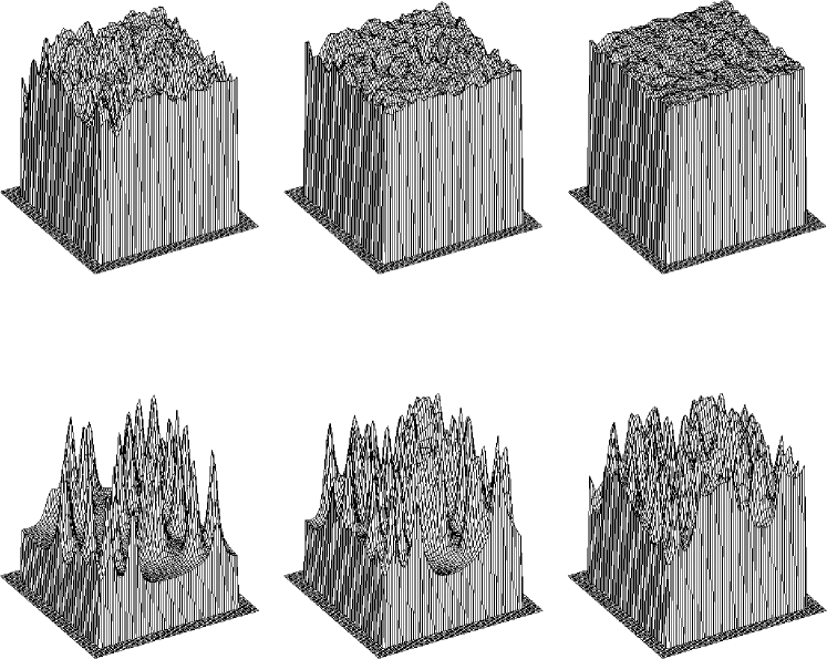
Figure 15: The height of these surfaces represents the image quality on a scale of $0-4\times$ the uncorrected quality as a function of position across the field for various number of telescopes. Each panel shows a region of sky about 1/4 degree on a side, and a telescope diameter $D=1.5$m and altitude $h=5$km were assumed. Lower left panel is for a single telescope and the other panels show the results of increasing the sampling density by a factor $N_{T}=2,4,8,16$ and $32$. The measure of image quality used is the normalized Strehl ratio, which is roughly proportional to the fraction of light contained within the diffraction limited PSF core. This was computed from the variance of the conditional mean centroid shift estimator. Modeling the effect of uncertainty in the predicted centroid as a convolution with a Gaussian ellipsoid we have found that the normalized Strehl is given approximately by Strehl $=3\times\exp(-\alpha/0.18)+1$ where $\alpha=\sigma^{2}/\sigma_{\rm total}^{2}$ is the fractional variance in the conditional mean, with $\sigma_{\rm total}^{2}$ is the unconstrained variance. The normalized Strehl ratio saturates at $S\simeq 4$ when the uncertainty in the centroid becomes small. To compute these images, for each pixel we identified the nearest $N\simeq 10$ stars, and used the theoretical deflection correlation functions to compute the $(2N+2)\times(2N+2)$ covariance matrix relating the 2 deflection components of the target point to those of the neighboring stars, and then inverted this to obtain the covariance matrix for the conditional mean.

Figure 15 can also be interpreted as giving the performance of a single telescope for a single deflecting layer at altitude $h=5N_{T}^{-1/2}$km. Thus, under favorable conditions one could expect to obtain good performance with a single instrument, but this would be the exception rather than the rule.

In this analysis only the instantaneous guide star deflections were used. Under the ‘frozen turbulence’ or ‘Taylor flow’ assumption there is more information at our disposal encoded in the history of the guide-star deflections, which provide a set of line-like samples of the deflection fields lying parallel to the wind direction. For a given target point, the most valuable information will come from those guide-stars lying up-wind and at a time lag given by the spatial separation divided by the wind speed. In the frozen turbulence assumption the mean number of such trails passing within say $\pm 1^{\prime}$ of a given point is roughly $n\Theta N_{T}$, where $n$ is the number density of guide stars, and $\Theta$ is the field size (using angular units of arc-minutes). For a field size of one degree and $n=(4^{\prime})^{-2}$ say, this we expect about $4N_{T}$ trails on average passing within a correlation length of a typical target point. For $N_{T}\sim 30$ this would give a very dense sampling rate. However, it may be over-optimistic, as it assumes that the turnover time for $\sim D$ sized eddies is as long as the time-scale for the layer to sweep across the whole field $\sim h\Theta/v$ which is several seconds. If the turnover time is shorter, then the correlations will decay more rapidly, and one should replace $\Theta$ in the sampling density estimate by the angular distance an eddy propagates in one turnover time. Anecdotal evidence suggests that the frozen turbulence approximation appears to be well obeyed over scales of several meters, so this would suggest that one should expect to obtain a substantial gain in sampling density by using temporal information. The improvement of image quality afforded by temporal history is shown in figure 16 assuming that the turbulence is effectively frozen for displacements of 5m and 10m respectively, corresponding to times of $0.5-1$s for wind speed of 10m/s. This is quite promising as it shows that even with a single telescope one can obtain good image quality over large areas of the sky, and that with just a few telescopes one should be able to obtain essentially full coverage. We caution, however, that this conclusion is strongly dependent on the assumption of a single deflecting screen.

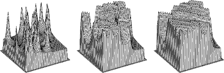
Figure 16: These surfaces show the variation of image quality for a single telescope, but using the time history of the deflection field under the ‘frozen-turbulence’ assumption. Vertical scale is as in figure 15. Left hand panel is for a single measurement, while center and right panels show the effect of using 5 and 10 measurements spaced by about 1m in physical separation, corresponding to a sampling rate of $10(v/10{\rm m/s}){\rm Hz}$.

In the calculations shown in figures 15, 16 the height of the deflecting layer was assumed known and the covariance matrix $M_{IJ}$ was computed from (33). In reality we would need to measure the covariance matrix from the actual measured guide star deflections. For a thin deflecting layer at height $h$ and moving with velocity ${\bf v}$ the deflection covariance function is

$$\langle\delta\theta_{i}({\bf x},\mbox{\boldmath$\theta$},t)\delta\theta_{j}({\bf x}^{\prime},\mbox{\boldmath$\theta$}^{\prime},t^{\prime})\rangle=c\xi_{ij}(\Delta{\bf x}+h\Delta\mbox{\boldmath$\theta$}+{\bf v}\Delta t)$$ (35)

where $\delta\mbox{\boldmath$\theta$}({\bf x},\mbox{\boldmath$\theta$},t)$ is the deflection of a guide star with position $\theta$ on the sky seen with a telescope at position ${\bf x}$ at time $t$, $\Delta{\bf x}\equiv{\bf x}-{\bf x}^{\prime}$ etc. and $c$ is a measure of the intensity of the layer. The covariance function can be estimated by averaging products of pairs of deflections. For a regular grid array of telescopes and uniform sampling in time, one obtains samples of the covariance on a uniform grid in $\Delta{\bf x}$, $\Delta t$ space, which is just what one needs. The sampling in angle space $\Delta\mbox{\boldmath$\theta$}$ is a little more problematic since the guide stars are randomly distributed, and yet one needs to evaluate the covariance at the angular separation between a guide star and the target object, which will not in general coincide with the separation between any particular pair of guide stars. To solve this one can bin the pairs into a grid of finite cells in $\Delta\mbox{\boldmath$\theta$}$ space and, if necessary, interpolate to obtain the covariance at the desired separation. This should not be too difficult. If one has say $N_{s}\sim 200$ guide stars on a $\Theta=1^{\circ}$ field then the number of pairs per $\sim(1^{\prime})^{2}$ correlation area is $\sim 5$ which should be adequate; the probability of having an empty cell if we bin into cells of $\sim 1^{\prime}$ size is very small, and interpolation over any patches should be fairly safe.

In principle, one could compute the covariance matrix for all pairs of observations and then invert the resulting matrix. Computing the full covariance matrix would be time consuming, but not insurmountably so. For $N_{s}=200$ guide stars, and $N_{T}=36$ telescopes, and if we keep a running history of say $N_{t}=32$ previous measurements then we have $(2N_{s}N_{T}N_{t})^{2}/2\sim 10^{11}$ pairs of measurements at any one time. Since the time history will be uniformly sampled the $\Delta t$ correlations can be performed with a FFT, and similarly for the $\Delta x$ correlations if the telescopes are laid out on a regular grid. With this simplification, the time complexity of the covariance matrix accumulation is essentially that of performing $N_{s}^{2}/2$ small ($N_{t}\times N_{T}$) FFTs every second or so which is not overwhelming since commercially available DSP devices perform FFTs at a rate of $\sim 50$M floating point data values per second. The real problem with this ‘sledgehammer’ approach is that to compute the conditional mean we will need to invert this huge $(2\times N_{T}\times N_{s}\times N_{t})^{2}$ matrix, which is prohibitively expensive in computational effort and is probably also numerically unstable. Luckily we do not need to do this. As discussed, the most valuable information pertaining to the deflection of a target object will come from the relatively small number of guide stars that are seen through the same patch of turbulence at some up-stream position. It is easy to identify which these observations are since they are those for which the correlation with the target object deflection is particularly strong, and so one need only work with the small subset of the full covariance matrix that involve these critical observations, and this greatly reduces the amount of computation. This was the approach used in computing figure 15 where only a subset of the guide stars were used for each pixel of the image.

The matrix inversion need only be done infrequently; on the rather long time-scale for macroscopic conditions such as wind speed, turbulence strength etc. to change. An instantaneous measurement of the covariance function will of course be noisy as we are sampling a single realization of a random process with finite extent in size and time. However, since the correlation time is on the order of the eddy turnover time of perhaps a few seconds, we can obtain statistically independent samples at intervals of order this time, so by averaging over several minutes say one should be able to determine the ensemble average covariance very accurately. The computation of the mean deflection needs to be done on a very short time-scale (a few tens of Hertz) but this is computationally a much easier task. A pleasant feature of this approach is that one can be fairly liberal in selection of guide stars; faint stars give more uncertain positions which therefore correlate less with other more precisely measured motions. The correlation matrix machinery ‘knows’ this and will automatically give these stars the weight they deserve.

Equation (31) provides the guide signal for the target cell of the detector. As discussed, in the Friedian approximation, the actual PSF is the PSF for perfect fast guiding convolved with a Gaussian ellipsoid $\exp(-{\bf x}\cdot{\bf m}^{-1}\cdot{\bf x}/2)$. This is useful since the image quality for a given patch of sky will vary from telescope to telescope and with position within the field, so (32) provides a useful criterion for rejecting or down-weighting poor images or sections thereof.

The procedure outlined above is somewhat inefficient in that it requires the computation of a fairly large matrix for each target. Neighboring target cells will tend to correlate strongly with the same set of guide stars, so the set of stars which correlate strongly with one or more of a cluster of neighboring cells will likely be not much larger than the set which correlate strongly with any individual cell. If so, then a great saving in computational effort can be made by computing the conditional probability for the deflections for the cluster of target cells at one go.

4.3 Multiple or Thick Turbulent Layers

The foregoing analysis was somewhat idealized in that a single thin layer of turbulence was assumed. If there are multiple or thick layers then the situation is somewhat more complicated. Nonetheless, given the huge amount of information at our disposal we believe that the conditional probability approach should still work, though depending on the nature of the turbulence there may be non-trivial constraints on the layout of the telescope array.

Consider first the case of a single thick layer at high altitude. The procedure outlined in the previous section will then fail if the baselines between the telescopes are too large. The problem is that the deflection for a target object at the zenith say will sample a vertical tube through the layer while a guide star seen from a different telescope at distance $\Delta{\bf x}$ will sample a tube which is inclined at an angle $\sim\Delta{\bf x}/h=\Delta\mbox{\boldmath$\theta$}$, and even if these two tubes overlap exactly in the center of the layer the deflections will tend to decohere if the thickness of the layer exceeds the value $\delta h\sim Dh/\Delta x$. Unfortunately, the observational situation is somewhat unclear as e.g. SCIDAR measurements tend to be limited in height resolution. For a width $\delta h\sim 100$m say, and $h\sim 5$km this implies the constraint on the size of the array $L\mathrel{\raise 1.29167pt\hbox{$<$}\mkern-14.0mu\lower 2.58334pt\hbox{$\sim$}}Dh/\delta h\simeq 50D\sim 75$m. This is not very restrictive. A further possible complication is wind shear across a thick layer which will tend to modify the deflection correlations.

Now consider multiple deflecting layers. According to the admittedly rather patchy observational studies reviewed above, one quite common situation is for there to be an additional strong component of seeing coming from the planetary boundary layer and from the immediate environment of the telescope, the so-called ‘dome seeing’. This is quite easy to deal with since it causes a common deflection for all of the guide stars for each telescope. If we simply take the mean deflection and subtract this, provided we have numerous guide stars and a sufficiently wide field then the residual guide star deflections after we subtract the mean should be essentially those due to the high altitude turbulent layer alone, and we can proceed as before. There are other means at ones disposal to further reduce the effect of low level turbulence. Very low level refractive index fluctuations can be homogenized by means of louvred enclosures and/or fans. The telescopes here are light and are auto-guiding, so it is not unreasonable to consider some kind of elevated support to raise them above very low level seeing. Also, since the isoplanatic angle for low level seeing is very large one can consider doing higher order wavefront correction with a deformable secondary. One way to implement this would be to augment the individual telescopes with smaller telescopes deployed around the periphery of the primary mirror which measure the average deflection of say a few tens of bright guide stars within the field. By taking the average, one effectively isolates the effect of the dome and boundary layer, and one can show that with say 6 such auxiliary telescopes --- which provide an extra 12 constraints in the form of samples the peripheral wavefront tilt --- one can effectively negate the effect of even quite strong low-level seeing. Provided low level seeing can be effectively eliminated by one or other of these approaches, one would then tune the aperture of the main telescopes such that they have diameter 4 times the $r_{0}$ for the ‘free-atmosphere’ seeing alone, as we have assumed above.

More difficult is the case where there are two or more high altitude layers giving a significant and comparable contribution to the deflection. It would be tempting to argue that since the strength of individual layers appears to have a highly non-Gaussian distribution with large dynamic range, having several layers of very similar strength is statistically improbable. However, this is probably over-complacent for the following reason: In the scheme outlined above, and with a relatively weak secondary deflecting layer, the correlation machinery will ‘lock on’ to the primary layer, with the net result that the sharp corrected image will get convolved with the natural seeing PSF for the second level. This can result in a significant loss of image quality even for a rather weak secondary layer. As a specific example, a secondary layer contributing only 4% of the total deflection power produces a reduction in Strehl of about 25%, so it is clearly highly desirable to have a guiding algorithm which can cope with multiple layers.

The problem here is not lack of information; with tens of telescopes, hundreds of guide stars and many time-steps in the history of the deflections one has a huge amount of information with which one should be able to separate the effects of multiple layers. In principle one could simply compute and invert the full covariance matrix to obtain the conditional deflection. Indeed, a rather nice feature of this sledgehammer approach is that there is then no need to try to solve for a set of discrete layer heights and intensities; the probability engine takes care of it automatically, as all the relevant information is encoded in the covariance matrix that one measures. The real problem here is how to decipher the information in a realistic amount of time. For a single layer it is relatively easy to identify and isolate a relatively small number of critical measurements which have a bearing on a given target object deflection. For multiple layers this is not the case, and a different approach is required.

What is needed is some way to at least approximately diagonalize the covariance matrix, so that one can avoid having to invert it all at once. Given the statistical translational invariance of the Gaussian random deflection screens we are dealing with, a natural approach is to work in Fourier space. Let us assume that we have a set of discrete deflecting layers at heights $h$, streaming across the field with velocities ${\bf v}_{h}$, and let us model the deflection field (which we will denote by ${\bf f}$ here) as a function of telescope position ${\bf x}$, angular position $\theta$ and time $t$ as

$${\bf f}({\bf x},\mbox{\boldmath$\theta$},t)=\sum\limits_{h}{\bf f}_{h}({\bf x}+h\mbox{\boldmath$\theta$}+{\bf v}_{h}t,t).$$ (36)

In the perfect frozen flow limit ${\bf f}_{h}$ would depend on time only implicitly through the spatial coordinate ${\bf x}+h\mbox{\boldmath$\theta$}+{\bf v}_{h}t$. The inclusion of an explicit dependence of ${\bf f}_{h}$ on time $t$ here allows for the evolution of the deflection field due to the turnover of eddies, though as discussed, we expect that the explicit time dependence will be rather slow as compared to the typical induced time dependence due to the motion of the screen. The deflection field is a random function of position and time and can be expressed as a Fourier synthesis

$${\bf f}_{h}({\bf x},t)=\int{d^{2}k\over(2\pi)^{2}}{d\omega\over 2\pi}\tilde{\bf f}_{h}({\bf k},\omega)e^{-i({\bf k}\cdot{\bf x}+\omega t)}$$ (37)

where the statistical homogeneity, stationarity and isotropy of the individual phase screens and their assumed mutual independence implies that distinct Fourier modes are statistically independent:

$$\langle\tilde{f}_{hi}({\bf k},\omega)\tilde{f}^{*}_{h^{\prime}j}({\bf k}^{\prime},\omega^{\prime})\rangle=(2\pi)^{3}\delta_{hh^{\prime}}\delta_{ij}\delta({\bf k}-{\bf k}^{\prime})\delta(\omega-\omega^{\prime})P_{h}(k,\omega)$$ (38)

where $P_{h}(k,\omega)$ is the spatio-temporal power spectrum of the layer at height $h$, and reality of ${\bf f}_{h}({\bf x},t)$ imposes the symmetry $\tilde{\bf f}_{h}(-{\bf k},-\omega)=\tilde{\bf f}_{h}^{*}({\bf k},\omega)$. For Kolmogorov turbulence the spatial power spectrum $P_{h}(k)\equiv\int d\omega\;P_{h}(k,\omega)$ is a power law $P_{h}(k)\propto k^{-5/3}$ at low spatial frequencies, with the smoothing with the telescope pupil introducing a high-$k$ cut-off at $k\sim 1/D$. Kolmogorov theory also tells us that the typical eddy velocity scales as the $1/3$ power of the eddy size, or equivalently as $v\propto k^{-1/3}$, so the width of $P_{h}(k,\omega)$ in temporal frequency must scale as $\omega_{*}(k)\sim v/L\propto k^{2/3}$. An acceptable model for $P_{h}(k,\omega)$ for a thin layer of turbulence is then

$$P_{h}(k,\omega)=P_{h}\Gamma({\bf k},\omega)\quad\quad{\rm with}\quad\quad\Gamma({\bf k},\omega)=k^{-5/3}\tilde{T}^{2}(k)\zeta(\omega/\omega_{*})/\omega_{*}(k)$$ (39)

with $\omega_{*}(k)=\omega_{D}(kD)^{2/3}$ and where $\tilde{T}(k)^{2}$ is the Fourier transform of the telescope pupil, which, for a simple filled circular aperture, is the ‘Airy-disk’ function. This model is parameterized by an overall intensity $P_{h}$ and by $\omega_{D}$ which is the turnover time for eddies of spatial frequency $k\sim 1/D$. The function $\zeta(y)$ is dimensionless, bell-shaped, and of unit width, which we take here to be approximately Gaussian. In 3-dimensional ${\bf k}-\omega$ space the model (39) is a disk of with axis parallel to the $\omega$-axis, radius $k_{*}\sim 1/D$, and with scale height $\omega_{*}(k)$. The assumed Gaussian form of the vertical profile $\zeta$ here is crude guess, and one would want to modify this in the light of either empirical observations and/or more sophisticated theoretical modeling.

Consider a particular telescope at position ${\bf x}_{0}$ and at the present time, which we take to be $t=0$, and define the angular transform of the deflection at angular frequency $\kappa$ as ${\bf f}_{0}(\mbox{\boldmath$\kappa$})\equiv\int_{\Theta}d^{2}\theta\;{\bf f}({\bf x}_{0},\mbox{\boldmath$\theta$},t=0)e^{i\mbox{\boldmath$\kappa$}\cdot\mbox{\boldmath$\theta$}}$, where the subscript $\Theta$ on the integral indicates that the integration is taken over the field of size $\Theta$. Using (36), (37) we can express ${\bf f}_{0}(\mbox{\boldmath$\kappa$})$ in terms of the spatio-temporal Fourier mode coefficients as

$${\bf f}_{0}(\mbox{\boldmath$\kappa$})=\sum\limits_{h}\int{d^{2}k\over(2\pi)^{2}}{d\omega\over 2\pi}\tilde{\bf f}_{h}({\bf k},\omega)e^{-i{\bf k}\cdot{\bf x}_{0}}\overline{W}_{\theta}(\mbox{\boldmath$\kappa$}-h{\bf k})$$ (40)

where $\overline{W}_{\theta}(\mbox{\boldmath$\kappa$})\equiv\int_{\Theta}d^{2}\theta\;e^{i\mbox{\boldmath$\kappa$}\cdot\mbox{\boldmath$\theta$}}$. If we take the field to be a square of side $\Theta$ then this is a 2-dimensional sinc function:

$$\overline{W}_{\theta}(\mbox{\boldmath$\kappa$})=\Theta^{2}{\sin^{2}\Theta\kappa_{x}/2\over(\Theta\kappa_{x}/2)^{2}}{\sin^{2}\Theta\kappa_{y}/2\over(\Theta\kappa_{y}/2)^{2}}$$ (41)

This function has a ‘central lobe’ at $\mbox{\boldmath$\kappa$}=0$ of height $\Theta^{2}$ and width $\delta\kappa\sim 1/\Theta$ flanked by side lobes of oscillating sign which diminish rapidly with increasing $\kappa$, so ${\bf f}_{0}(\mbox{\boldmath$\kappa$})$ depends only on those Fourier modes in a small range of spatial frequency of size $\delta k\sim 1/h\Theta$ around ${\bf k}=h\mbox{\boldmath$\kappa$}$, this being the spatial frequency which maps to the chosen angular frequency $\kappa$ at altitude $h$. If $h\Theta>L$ then the complex phase factor $e^{-i{\bf k}\cdot{\bf x}_{0}}$ in (40) is nearly constant and so ${\bf f}_{0}(\mbox{\boldmath$\kappa$})$ is the product of $\tilde{f}({\bf k},\omega)$ with a cylindrical window function which is infinitely long in $\omega$ and has width $\delta k\sim 1/h\Theta$. If on the other hand $h\Theta<L$ then the variation of the phase factor is appreciable for typical ${\bf x}_{0}\sim L$ and the window function has oscillatory modulation with scale length $\sim 1/L$.

Similarly, if we define the 5-dimensional Fourier transform of the measured deflections as

$${\bf F}({\bf k},\mbox{\boldmath$\kappa$},\omega)=\sum\limits_{{\bf x},\mbox{\boldmath$\theta$},t}{\bf f}({\bf x},\mbox{\boldmath$\theta$},t)e^{i({\bf k}\cdot{\bf x}+\mbox{\boldmath$\kappa$}\cdot\mbox{\boldmath$\theta$}+\omega t)}$$ (42)

then, in terms of the transform of the deflection screens $\tilde{\bf f}_{h}({\bf k},\omega)$, this is

$${\bf F}({\bf k},\mbox{\boldmath$\kappa$},\omega)=\sum\limits_{h^{\prime}}\int{d^{2}k^{\prime}\over(2\pi)^{2}}{d\omega^{\prime}\over 2\pi}\tilde{\bf f}_{h}({\bf k}^{\prime},\omega^{\prime})W_{x}({\bf k}-{\bf k}^{\prime})W_{\theta}(\mbox{\boldmath$\kappa$}-h{\bf k}^{\prime})W_{t}(\omega-\omega^{\prime}-{\bf k}^{\prime}\cdot{\bf v}_{h^{\prime}})$$ (43)

where $W_{x}({\bf k})\equiv\sum_{\bf x}e^{i{\bf k}\cdot{\bf x}}$ is the Fourier transform of the telescope array; $W_{\theta}(\mbox{\boldmath$\kappa$})\equiv\sum_{\theta}e^{i\mbox{\boldmath$\kappa$}\cdot\mbox{\boldmath$\theta$}}$ is the transform of the guide star distribution and $W_{t}(\omega)=\sum_{t}e^{i\omega t}$ is the transform of the of the temporal sampling pattern. Now all of these functions are quite strongly peaked at zero argument, $W_{x}$ has width $\delta k$ of order the inverse of the telescope array size $L$, $W_{\theta}$ has width $\delta\kappa\sim 1/\Theta$ (like $\overline{W}_{\theta}$) and $W_{t}$ has width $\delta\omega$ equal to the inverse of the time period $T$ over which we choose to integrate. Consequently, and like ${\bf f}_{0}(\mbox{\boldmath$\kappa$})$, ${\bf F}({\bf k},\mbox{\boldmath$\kappa$},\omega)$ receives a large contribution from a restricted region of spatial frequency around ${\bf k}^{\prime}\simeq{\bf k}$. Unlike ${\bf f}_{0}(\mbox{\boldmath$\kappa$})$ however, the contribution to ${\bf F}({\bf k},\mbox{\boldmath$\kappa$},\omega)$ is also restricted in altitude and temporal frequency since for the argument of $W_{\theta}$ to be small requires both that $\kappa$ point in approximately the same direction as ${\bf k}$ and that the ratio of angular to spatial frequency $\kappa/k$ should coincide with the altitude of an actual layer of turbulence. Finally, ${\bf F}(h,{\bf k},\omega)$ is most sensitive to temporal frequencies of the deflection screen $\omega^{\prime}\simeq\omega-{\bf k}\cdot{\bf v}_{h}$ which means, if we assume that the intrinsic deflection screen evolution time-scale is long compared to $D/v$, that ${\bf F}({\bf k},\mbox{\boldmath$\kappa$},\omega)$ is only sensitive to a screen at altitude $h$ if the screen velocity satisfies $|{\bf k}\cdot{\bf v}_{h}-\omega|\leq\omega_{*}$, where $\omega_{*}$ is on the order of the inverse of the eddy turnover time.

Equations (40) and (43) above give ${\bf f}_{0}(\kappa)$ and ${\bf F}({\bf k},\mbox{\boldmath$\kappa$},\omega)$ respectively as integrals of $\tilde{\bf f}_{h}({\bf k},\omega)$ times some window function. However, the window function for ${\bf F}({\bf k},\mbox{\boldmath$\kappa$},\omega)$ is in all dimensions at least as narrow as the window function for ${\bf f}_{0}(\kappa)$, and therefore ${\bf f}_{0}(\mbox{\boldmath$\kappa$})$, from which we can trivially extract the desired guide signal ${\bf f}({\bf x}_{0},\mbox{\boldmath$\theta$},t=0)$ by inverse transforming, should be well constrained by measurements of ${\bf F}({\bf k},\mbox{\boldmath$\kappa$},\omega)$ taken at appropriate spatial, angular and temporal frequencies. Since these are both linear functions of $\tilde{\bf f}({\bf k},\omega)$ they should have Gaussian statistics, and so one can write down the conditional probability

$$p({\bf f}_{0}(\mbox{\boldmath$\kappa$})|{\bf F}({\bf k}^{\prime},\mbox{\boldmath$\kappa$}^{\prime},\omega^{\prime}),{\bf F}({\bf k}^{\prime\prime},\mbox{\boldmath$\kappa$}^{\prime\prime},\omega^{\prime\prime})\ldots)$$ (44)

from which one can determine the conditional mean value of ${\bf f}_{0}(\mbox{\boldmath$\kappa$})$, very much as was done before for a single deflecting layer. Let us assume for the moment that $P_{h}({\bf k},\omega)$ and the velocities ${\bf v}_{h}$ are known. If so, the covariance matrix in the multi-variate Gaussian distribution (44) has components like

$$\matrix{\langle f^{*}_{0i}(\mbox{\boldmath$\kappa$}^{\prime})F_{j}({\bf k},\mbox{\boldmath$\kappa$},\omega)\rangle=\cr\delta_{ij}\sum\limits_{h}\int{d^{2}k^{\prime}\over(2\pi)^{2}}{d\omega^{\prime}\over 2\pi}P_{h}(k^{\prime},\omega^{\prime})e^{-i{\bf k}^{\prime}\cdot{\bf x}_{0}}W_{x}({\bf k}-{\bf k}^{\prime})W_{\theta}(\mbox{\boldmath$\kappa$}-h{\bf k}^{\prime})W_{t}(\omega-\omega^{\prime}-{\bf k}^{\prime}\cdot{\bf v}_{h})\overline{W}_{\theta}^{*}(\mbox{\boldmath$\kappa$}^{\prime}-h{\bf k}^{\prime})}$$ (45)

Since the various window functions here are known and compact, it is straightforward to enumerate the limited number of 5-dimensional transform modes which are relevant for any given $\kappa$, evaluate the appropriate covariance matrix and thereby obtain an accurate conditional mean estimator for ${\bf f}_{0}(\mbox{\boldmath$\kappa$})$ as a linear combination of a limited subset of the ${\bf F}({\bf k},\mbox{\boldmath$\kappa$},\omega)$ values.

To implement this program we need some way of determining $P_{h}(k,\omega)$. If we evaluate ${\bf F}({\bf k},\mbox{\boldmath$\kappa$},\omega)$ at $\mbox{\boldmath$\kappa$}=h{\bf k}$, square it and take the expectation value: $P_{F}(h,{\bf k},\omega)\equiv\langle{\bf F}({\bf k},h{\bf k},\omega)\cdot{\bf F}^{*}({\bf k},h{\bf k},\omega)\rangle$, then from (38), (43) we have

$$P_{F}(h,{\bf k},\omega)={N_{t}^{2}\over\tau}\sum\limits_{h^{\prime}}{d^{2}k^{\prime}\over(2\pi)^{2}}P_{h^{\prime}}(k^{\prime},\omega-{\bf v}_{h^{\prime}}\cdot{\bf k}^{\prime})W_{x}^{2}({\bf k}-{\bf k}^{\prime})W_{\theta}^{2}(h{\bf k}-h^{\prime}{\bf k}^{\prime})$$ (46)

where we have taken the integration time to be greater than the eddy turnover time-scale to effect an integration over spatial frequency. As already discussed, a layer of turbulence has a spatio-temporal power spectrum which is a flaring disk of thickness $\omega_{*}$ so the quantity $P_{h}(k,\omega-{\bf v}_{h}\cdot{\bf k})$ appearing above is also a disk, but is inclined with respect to the $\omega=0$ plane with mid-plane gradient $d\omega/dk=v$. Furthermore, if the $D$-sized eddy turnover time is much less than the translation time-scale $D/v$, as the observations indicate, then $\omega_{*}\ll vk_{*}$, so the vertical displacement of the disk is large compared to its thickness. If $h$ coincides with an actual deflecting layer, and if we consider for the moment only the contribution from that layer $h^{\prime}=h$, then $P_{F}(h,{\bf k},\omega)$ is a 2-dimensional convolution of this thin tilted disk with the function $W_{x}^{2}({\bf k})W_{\theta}^{2}(h{\bf k})$. Now this function has width $\delta k\sim{\rm min}(1/L,1/h\Theta)$ whereas the intersection of the inclined disk with a plane $\omega=$ constant has width $\Delta k\sim\omega_{*}/v$ so provided $\omega_{*}\gg v/{\rm max}(L,h\Theta)$ (i.e. the eddy turnover time is short compared to the time-scale for the eddy to be convected across either the entire field or the overall extent of the array, whichever is greater) then $\Delta k\gg\delta k$ and the convolution has little effect and therefore

$$P_{F}(h,{\bf k},\omega)\simeq P_{h}(k,\omega-{\bf v}_{h}\cdot{\bf k})$$ (47)

and one can determine $P_{h}({\bf k},\omega)$ by fitting for inclined versions of disk models of the form (39) directly to the measured power spectrum $P_{F}(h,{\bf k},\omega)$ One particularly simple way to achieve this would be to compute

$$P(h,{\bf v})\equiv\int d^{2}k\int d\omega\;\Gamma({\bf k},\omega-{\bf k}\cdot{\bf v})P_{F}(h,{\bf k},\omega)$$ (48)

the local maxima of which should coincide with the heights, velocities of the various layers.

It is important in what follows to have a clear picture of the form of the power spectrum $P_{F}(h,{\bf k},\omega)$ which, being four dimensional, is somewhat difficult to visualize. To this end, imagine you are sitting in the control room of a wide field imaging array. Measurements of guide star deflections have been recorded and transformed to produce $F({\bf k},\mbox{\boldmath$\kappa$},\omega)$ and you are viewing a graphics device with a 3-D renderer displaying an isodensity surface of the measured power $P_{F}(h,{\bf k},\omega)$ in ${\bf k}$, $\omega$ space, integrated over perhaps ten minutes or so, for a given altitude $h$. A widget on the screen allows you to control the altitude. At first you see nothing. As you slowly vary the altitude suddenly a disk like structure springs into view, as shown schematically in figure 17. The radial extent of the disk has an Airy disk form as given by the model (39), and it has the expected bell-shaped vertical profile. Wiggling the altitude control you estimate that the width of this structure is $\delta h\sim D/\Theta$. This is the signature of a horizontally convecting layer of seeing. The disk is tilted (actually sheared), from which you can read off the wind velocity vector, and the thickness tells you how fast it is evolving internally. Further variation of the altitude reveals a number of further layers with different strengths and velocities and perhaps thicknesses, but otherwise matching the pre-determined template.

Figure 17: Schematic illustration of the spatio-temporal power spectrum for a streaming turbulent layer. As discussed in the text, a slowly evolving layer of turbulence has an intrinsic power spectrum $P_{h}({\bf k},\omega)$ which is a disk-like function extending to $|k|\simeq 1/D$ in the spatial direction and with thickness $\omega_{*}\sim 1/t_{D}$ in the temporal direction (vertical in the figure). The measured power spectrum $P_{F}(h,{\bf k},\omega)$, with $h$ taken to be the height of some layer streaming with velocity ${\bf v}$, is similar, but tilted slightly as illustrated, with the tip of the normal to the disk being displaced from the vertical axis in the direction ${\bf v}$. Not shown in this figure is the power aliased from different layers $h^{\prime}\neq h$. The aliased power consists of a periodic array of weak ‘ghost’ disks, tilted in the appropriate directions, and with centers on a grid of points in the $k_{x}$, $k_{y}$ plane with spacing $2\pi/\Delta x$ where $\Delta x$ is the spacing of the telescopes in the array.

Results of the kind described would lend credence to the idea that the behaviour of the atmosphere can indeed be characterised by a tiny subset of all the Fourier components computed, and that the Fourier transform of the actual deflection at the present instant ${\bf f}_{0}(\mbox{\boldmath$\kappa$})$ may be accurately given by a linear combination of a small set of ${\bf F}({\bf k},\mbox{\boldmath$\kappa$},\omega)$ values, and that this might allow one to freeze out the motion of all the images in the field. However, the display device also has a widget to control the level of the isodensity contour plotted. As you increase the contrast the picture changes radically. The disk centered on the origin swells as expected, but rather suddenly a set of additional low level structures appear laid out on a grid in the $\omega=0$ plane. The spacing of these structures is $\delta k=2\pi/\Delta x$ where $\Delta x$ is the spacing of the telescopes --- so the spacing is small compared to the extent of the disk --- and on closer inspection they are seen to be well modeled by superpositions of weak replicas of the disks seen in the high iso-surface level scan, but with seemingly random strengths. This background of low level ghost images also persists when you tune the altitude control to arbitrary positions.

What is happening here is aliasing of deflection power from spatial frequencies differing from the target frequency by integer multiples of $2\pi/\Delta x$, and from different heights $h^{\prime}\neq h$. In the foregoing we have assumed that $W_{x}$, $W_{\theta}$ are narrow functions of their arguments, and we have approximated the values of various integrals by simply integrating over the ‘central lobe’ of these functions. This is a good first approximation to be sure, but in fact both of these functions have extended side-lobes. For a regular grid telescope array, $W_{x}({\bf k})$ has the form of a 2-dimensional sinc function with central value $W_{x}(0)=N_{T}^{2}$ and width $\delta k\sim 1/L$ but this pattern repeats with period $2\pi/\Delta x$. Similarly, $W_{\theta}^{2}$ has a central lobe of height $N_{s}^{2}$ and width $\delta\kappa\sim 1/\Theta$, but for $|\kappa|\gg 1/\Theta$ the function $W_{\theta}(\mbox{\boldmath$\kappa$})=\sum e^{i\mbox{\boldmath$\kappa$}\cdot\mbox{\boldmath$\theta$}}$ is effectively the sum of $N_{s}$ random plane waves with random phases, so it resembles a Gaussian random field with coherence length $\delta\kappa\sim 1/\Theta$ and with mean square value $W^{2}_{\theta}(\mbox{\boldmath$\kappa$})=N_{s}$. These weak but extended side-lobes will alias power from different spatial frequencies ${\bf k}^{\prime}\neq{\bf k}$ and from different layers $h^{\prime}\neq h$ into ${\bf F}({\bf k},h{\bf k},\omega)$ but not into ${\bf f}_{0}(\mbox{\boldmath$\kappa$})$. This leakage of power will result in imprecision in the conditional mean estimator.

To understand the conditions for obtaining an accurate deflection model let us assume that we have correctly identified the the strengths and velocities of the deflecting layers, and that we have computed ${\bf F}({\bf k},h{\bf k},\omega)$ for a spatial frequency ${\bf k}\sim 1/D$ and a temporal frequency lying within a particular layer; i.e. for a point lying within the disk shown in figure 17. The key question is what fraction of ${\bf F}({\bf k},h{\bf k},\omega)$ actually arises within the layer at the height $h$ and what fraction is aliased from entirely different layers? We can infer the answer to this question from inspection of equation (46). This integral will have a central lobe or ‘primary’ contribution and an integrated side-lobe or ‘aliased’ contribution. The primary contribution comes from ${\bf k}^{\prime}\simeq{\bf k}$ and is $\sim P_{h}W_{x}^{2}(0)W_{\theta}^{2}(0)\delta k^{2}$ or

$$P_{F}({\rm primary})\simeq P_{h}N_{s}^{2}N_{T}^{2}\;{\rm min}(1/L^{2},1/h^{2}\Theta^{2})$$ (49)

(we have ignored the prefactor $N_{t}^{2}/\tau$). The periodic form of $W_{x}^{2}({\bf k})$ results in a series of ‘ghost images’ of the power for all of the discrete layers, each with the appropriate tilt, and replicated on a periodic grid in ${\bf k}$ with spacing $\Delta k=2\pi/\Delta x$. The aliased power therefore appears where ${\bf k}-{\bf k}^{\prime}\simeq{\bf n}\Delta k$, where ${\bf n}$ is a vector with integer values components. These aliased contributions are individually weak, because typically the argument of $W_{\theta}$ will be large compared to $1/\Theta$ so $W_{\theta}\simeq N_{s}$ rather than $N_{s}^{2}$. If there are $N_{l}$ layers then there will be $\sim N_{l}\times(k/\Delta k)^{2}=N_{l}(\Delta x/D)^{2}$ ghost images located within the region of interest which is of size $k\sim 1/D$, so they are quite numerous. On the other hand, the probability that a given point ${\bf k}$, $\omega$ falls within any one of these ghost images is $\sim D/{\rm max}(D,vt_{D})$ which is small if $vt_{D}\gg D$ which we expect to be the case. Putting all these factors together we find for this integrated aliased power

$$P_{F}({\rm aliased})\simeq P_{h}N_{s}N_{T}^{2}(1/L^{2})\;{\rm max}(1,D/vt_{D})(\Delta x/D)^{2}$$ (50)

where we have assumed that the velocities of the distinct layers are randomly distributed. Aliasing will be stronger from another layer which has nearly the same velocity, but this is an unlikely situation. The requirement that the primary contribution to $F(h{\bf k},{\bf k},\omega)$ (which correlates strongly with the thing we are trying to predict) greatly exceed the aliased contribution (which doesn’t) is then simply

$$N_{s}N_{T}D\;{\rm max}(D,vt_{D})\gg N_{l}\;{\rm max}(L^{2},h^{2}\Theta^{2}).$$ (51)

This is a key result of this section and is physically very reasonable. The RHS is the total area of all of the deflecting layers, whereas the LHS is the total area of the samples of the deflection provided by $N_{s}$ guide stars seen through $N_{T}$ telescopes. For aliasing to be unimportant we need to sample the layers sufficently well.

Equation (51) provides the following important constraint on the configuration of the array: one should not choose $L$ to be much greater than $h\Theta$, which is about 100m for our canonical $h=5$km and a $\Theta=1$ degree field. Primarily this is because taking $L\gg h\Theta$ would unneccessarily increase the total area of deflection screen that one must deal with. This equation suggests that aliasing is independent of the array size for smaller $L$. However, this is not the whole story. What we have neglected here is the possibility of aliasing of power in (46) from a nearby layer $h^{\prime}=h+\Delta h$ through the central lobe of $W_{x}^{2}$. Imagine we have taken $L$ to be very small so the array is compact. That means that the transform of the array $W_{x}^{2}$ will be correspondingly wide, with width $\delta k\sim 1/L$, so in (46) the factor $W_{x}({\bf k}={\bf k}^{\prime})$ will limit the contribution to the integral to a small region of size $\sim 1/L$ around ${\bf k}^{\prime}={\bf k}$. More restrictive however is the factor $W_{\theta}^{2}(h{\bf k}-h^{\prime}{\bf k}^{\prime})$ which clearly has a narrow peak for $h^{\prime}=h$ of width $\delta k\sim 1/h\Theta$ around ${\bf k}^{\prime}={\bf k}$. However, there will also be secondary peaks of $W_{\theta}^{2}$ centered on ${\bf k}^{\prime}=(h/h^{\prime}){\bf k}$, and these will fall within the more extended central lobe of $W_{x}^{2}$ if $\Delta h/h\mathrel{\raise 1.29167pt\hbox{$<$}\mkern-14.0mu\lower 2.58334pt\hbox{$\sim$}}\delta k/k\sim D/L$. This would be problematic: according to (40) ${\bf f}_{0}(\mbox{\boldmath$\kappa$})$ receives a contribution from each layer which is restricted to a region of size $\delta k\sim 1/h\Theta$ around ${\bf k}=\mbox{\boldmath$\kappa$}/h$ whereas for $L\mathrel{\raise 1.29167pt\hbox{$<$}\mkern-14.0mu\lower 2.58334pt\hbox{$\sim$}}Dh/\delta h$, the measured $F({\bf k},h{\bf k},\omega)$ receives comparable contributions from neighboring regions and this will destroy the precision of our conditional mean estimate for ${\bf f}_{0}(\mbox{\boldmath$\kappa$})$. This is slightly over-pessimistic since the contribution from these secondary layers may in fact be suppressed if their velocity difference is such that ${\bf k}\cdot\Delta{\bf v}>D\omega_{*}$. This will usually be the case if the internal evolution time-scale is small compared to the convection time-scale, and if $\Delta{\bf v}\sim{\bf v}$, but this cannot be guaranteed, and in any case there will still be a range of ${\bf k}$ values (lying perpendicular to $\Delta{\bf v}$) for which the confusion cannot be resolved. The solution to this problem is straightforward: choose an array size $L$ which is satisfies $L\mathrel{\raise 1.29167pt\hbox{$>$}\mkern-14.0mu\lower 2.58334pt\hbox{$\sim$}}Dh/\Delta h$. For a separation $\Delta h=300$m say this gives $L\mathrel{\raise 1.29167pt\hbox{$>$}\mkern-14.0mu\lower 2.58334pt\hbox{$\sim$}}25$m.

There is a simple way to understand this latter constraint. What we are doing here is disentangling the deflections from distinct layers by evaluating the 5-dimensional transform ${\bf F}({\bf k},\mbox{\boldmath$\kappa$},\omega)$ at the angular frequency $\mbox{\boldmath$\kappa$}=h{\bf k}$ coresponding to a spatial frequency ${\bf k}$ at height $h$. If we use too small an array then we have poor resolution in spatial frequency $\delta k\sim 1/L$ and this converts to a corresponding lack of resolution in height. This harks back to the observation made at the start of this section, that a layer of thickness $\delta h$ is only effectively thin if $L\mathrel{\raise 1.29167pt\hbox{$<$}\mkern-14.0mu\lower 2.58334pt\hbox{$\sim$}}Dh/\delta h$. Thus, if the nature of the refractive index fluctuations is slowly evolving (and therefore highly predictable) streaming layers of thickness $\delta h$ with separation $\Delta h$ then we want to be able to resolve the separate layers. If we fail to resolve two layers moving with different velocities, then we obtain a single effective layer with enhanced width in temporal frequency, which consequently has less predictable evolution. On the other hand, we do not want to resolve the individual layers further into sub-layers. If we take $\delta h=100$m and $\Delta h=300$m then this would argue for an array size $L\sim 50$m or so, this choice also being consistent with the independent constrain that $L\mathrel{\raise 1.29167pt\hbox{$<$}\mkern-14.0mu\lower 2.58334pt\hbox{$\sim$}}h\Theta$.

These considerations answer a question that may have occurred to the reader. Why not retro-fit an existing 10m class telescope with some kind re-imaging optics with stops to generate sub-pupils and with an array of cameras to synthesise an array of 1.5m aperture telescopes? While this approach is attractive on grounds of cost, if the values $\delta h$, $\Delta h$ characterizing the stratification of seeing given above are at all accurate then such a design would be sub-optimal as compared to a purpose built array with larger baselines because it would be unable to resolve the separation between layers. In the context of (51) such an instrument would benefit from having a smaller effective number of layers $N_{l}$, but the short effective coherence time for the ‘composite’ layers $t_{D}\sim D/v$ would tend to outweigh this gain.

Returning to the case of an array, and assuming that the condition $L\mathrel{\raise 1.29167pt\hbox{$<$}\mkern-14.0mu\lower 2.58334pt\hbox{$\sim$}}h\Theta$ is satisfied, equation (51) becomes independent of the field size $\Theta$ since $N_{s}\propto\Theta^{2}$, and gives then the number of telescopes required to deal with a certain number of layers distributed over some range of heights. As already emphasised, the sensitivity of the image quality to imprecision of conditional deflection means that we want to satisfy the inequality (51) strongly, but even so we find equation (51) encouraging. The arguments leading to (51) are admittedly hand-waving, and it would be nice to quantify the dimensionless factors we have brushed over, but it is probably reasonable to scale from the case of a single layer which we have analysed quantitatively. As we saw in §4.2 for a high altitude ($h\sim 5$km) deflection layer a single layer is essentially fully constrained with $\sim 10$ telescopes even in the absence of useful temporal correlations. So it should not be too difficult to satisfy the condition (51) for realistic sized arrays. With say 30 telescopes one should be able to deal with several high altitude layers and even more layers at low altitude.

With more detailed knowledge for the properties of the atmosphere it should be possible to accurately compute the performance of this type of imaging system and predict the resulting image quality. This would then allow one to configure the telescope array to optimize the performance. Unfortunately the data that are currently available from SCIDAR studies etc. are sparse and do not necessarily address the key issues here such as what is the time-scale for the layers to evolve etc. What are critically needed are measurements of the deflection correlation function which sample the range of spatial, angular and temporal separations relevant here, and also over a period of time in order to properly understand the statistics of these meteorological processes. Some of these issues can be addressed simply with drift scan observations on small telescopes, or with measurements from wavefront sensors on $8-10$m class telescopes, but also needed are measurements with two or more telescopes (or with a single large telescope equipped with pupil stops and optics in order to simulate a number of small telescopes) in order to determine, for example, the decorrelation at large angular separations due to finite thickness of the deflecting layers. Experiments of this kind will be able to address the important, and to a large degree open, question of intermittency and non-Gaussianity of the atmospheric deflections. Given data of this kind one can then accurately establish the performance of the type of instrument we are proposing before embarking on construction.

5 Detectors

The detectors for this array of telescopes must be able to compensate for independent image motion on a scale of about 1 arc-minute, which for a field of view of about a degree requires 3--4000 independent image motion compensation elements. The other important consideration is that the detector must have many pixels (approximately $10^{9}$ per square degree for $0^{\prime\prime}.1$ pixels) for each of $\sim 36$ telescopes, so the detectors must be reasonably inexpensive.

Our proposed solution to these challenges is a monolithic device consisting of say a $30\times 30$ array of independently addressable $600\times 600$ pixel multi-directional or ‘orthogonal transfer’ CCDs [Tonry, Burke, & Schechter 1997]. With a pixel size of 5$\mu$m the resulting $18{\rm K}\times 18{\rm K}$ pixel device would measure $\sim$100mm$\times$100mm and would fill an entire 150mm diameter silicon wafer. With the optical system designed to deliver a plate scale of $0^{\prime\prime}.1/5\mu$m pixel, a $2\times 2$ array of $18{\rm K}\times 18{\rm K}$ OTCCDs butted together into a mosaic would provide the desired 1${}^{\rm o}\times 1^{\rm o}$ field subdivided into independently-controllable 1^′$\times$1^′ patches. Figure 18 illustrates this idea. The pixel size of $5\mu$m is a factor 3 times smaller than those commonly used in astronomical applications, but similar to the pixel sizes commonly used in consumer electronics applications. Should manufacturing considerations force one to larger pixels one would need to use a correspondingly larger array of chips to maintain the desired field of view, with corresponding increase in costs. The real limitations on physical pixel size is one of the major unknowns in costing and optimizing this system.

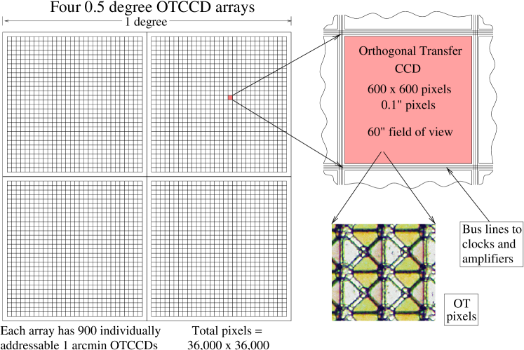
Figure 18: This schematic drawing illustrates the 1^o$\times$1^o focal plane of independently addressable OTCCDs. The focal plane consists of a 2$\times$2 array of $18{\rm K}\times 18{\rm K}$ OTCCD arrays each measuring $\sim$100mm on a side. Each of the small sub-cells measures $600\times 600$ pixels and corresponds to a $\sim 1^{\prime}\times 1^{\prime}$ patch on the sky. The gaps between sub-cells are the equivalent of $\sim$30 pixels and are needed to bus the various signals to the independent OTCCDs, and the larger gaps between the monolithic arrays are needed for wire bond pads and such.

In the subsequent sections we will describe how the OTCCD works and how it can answer our need for a ‘‘rubber focal plane’’, the new step of making a monolithic array of independent CCDs, how these arrays would be operated in practice, and finally some estimates of feasibility and yields.

5.1 The Orthogonal Transfer CCD

In any CCD the charge is localized into discrete pixels by application of potentials to adjacent electrodes (‘‘gates’’) which are separated from the charge collecting region by very thin layers of dielectric. A CCD is read out by systematically changing the gate potentials in such a way that the charge is moved laterally while maintaining each pixel’s identity by keeping at least one gate negative (potential maximum) between each pixel. A conventional 3-phase CCD achieves this by using permanent implants (‘‘channel stops’’) which divide the CCD into vertical columns and then three gates per pixel in the horizontal direction. This process of shifting the charge (‘‘parallel clocking’’) is essentially noiseless (extra ‘‘spurious’’ charge created by the process is typically unmeasurable for modest gate voltages), highly efficient (charge transfer inefficiency (CTI) is typically less than 1 part in $10^{5}$ or charge transfer efficiency $\hbox{CTE}=1-\hbox{CTI}>0.99999$), and extremely fast (rates of $10^{4}-10^{5}$ pixel/sec are common). There is no reason that this parallel clocking cannot take place while the CCD is collecting light, and indeed this is the basis of time-delay integration (TDI) or ‘‘drift scanning’’ where a field of view is moved steadily down a column and the CCD is read out at precisely the same rate so that the image is not blurred (e.g. the SDSS CCD mosaic array).

The Orthogonal Transfer CCD (OTCCD) goes one step further in discarding the permanent channel stop but introducing a fourth gate, and by making the layout of the gates symmetric to $90^{\circ}$ rotations. The OTCCD is therefore capable of tracking image motion in an arbitrary direction. As the optical image dances about over the CCD, the accumulating charge can be shifted in synchronism and any blurring from image motion will be removed. The device is bordered by a scupper which removes any charge which is shifted off of the array. Figure 19 shows how the charge is moved in such a device, either for transport to the serial register for readout or for tracking image motion, and the inset in figure 18 shows a photomicrograph of the gates of an actual device with 15$\,\mu$m pixels.

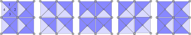
Figure 19: This diagram shows the gate layout of a symmetrical OTCCD pixel and illustrates how the charge is clocked to the right by successive application of negative (dark) or positive (light) potentials on the gates. The gray circles represent channel stops which prevent charge from moving between the corners of the triangular gates. The symmetry permits charge to be clocked left, right, up, down, or even diagonally.

This layout of gates also lends itself well to fractional pixel sub-stepping, which is important since we are expecting images with $0^{\prime\prime}.12$ FWHM and the pixel size is $0^{\prime\prime}.1$. Figure 20 shows how a collection pixel can be shifted by a fraction of a pixel.

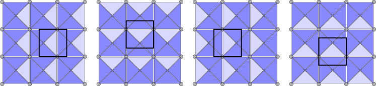
Figure 20: By setting one of the four gates positive (light), the effective location of a pixel can be shifted by a fraction of a pixel. The heavy black outline shows the region on the detector where photo-electrons will migrate to a common point. Other configurations using 2 or 3 positive gates are also possible, allowing quite fine control of the collection pixel position.

5.2 OTCCD Arrays

Making a monolithic mosaic array of OTCCDs should not present serious problems in design or manufacture. The overall layout of the array would have $30\times 30$ independent $600\times 600$ OTCCDs separated by gaps for common bus lines which might need to be as large as about 30 pixels or 3^′′, which is about a 10 percent effective dead area on the array.

The individually addressable OTCCDs would share common connections for a number of signals such as serial gates and amplifier drain and reset, but each must have independently addressable parallel gates (to effect the necessary shifts for each CCD) and independent amplifier outputs. This can be accomplished by equipping each CCD with a set of transistors which lie between these connections and the common bus lines. Using an x-y addressing scheme these transistors can be turned on or off and any individual CCD connected or disconnected from the external pins of the array.

As far as the external electronics is concerned, once 10 bits worth of x-y address has been decoded and the appropriate CCD activated, the array looks like a single, small CCD.

One challenge of making such an array work is that a CCD must maintain the potentials on its gates or else it cannot keep the charge within individual pixels. However, the x-y multiplexing means that all but one CCD is normally disconnected from the external drive electronics. We do not expect that this will be a problem, because the capacitance of CCD gates is such that they will maintain their potentials for many seconds after being disconnected. Thus, as long as the CCDs are each periodically reconnected to the external gate voltages they can continue to do their job. This mandates that the external electronics continuously ripple through the array, much like dynamic RAM. Since we need to visit each CCD ten or more times a second to apply shifts, and since we need many copies (perhaps 10 per array) of the external electronics for speed in acquiring guide star information, this should not be a problem.

A very significant advantage to this sort of CCD array is it is very tolerant of manufacturing defects that would otherwise destroy a large monolithic device. Typical wafer defects are very localized, so a defect that might render a conventional wafer-scale CCD unusable will only ruin a single $\sim$1^′$\times$1^′ subarray on the OTCCD array. Given that we are thinking of $\sim 36$ telescopes each with its own focal plane OTCCD arrays, the loss of a square arcminute from a single detector is negligible. Likewise the gaps between the CCDs will not appear in the image produced by the entire telescope array, since it is simple to offset the pointings of each telescope so that the gaps do not overlap.

5.3 Mosaic Operation

Some number of the CCDs in this array will contain sufficiently bright stars around which small patches will be read out for guiding information, thus sacrificing the rest of that 1^′$\times$1^′ cell for science. This can be done in ‘shutterless video’ mode and we have already demonstrated that it is possible to work at 100 Hz sampling with relatively slow electronics and relatively large CCDs on available guide stars (see §3).

An example of the observational strategy follows: first, one would identify the stars which are sufficiently bright to serve as guide stars and identify the $600\times 600$ pixel OTCCD cells which contain these guide stars. Then one would start the following observing sequence. First all the CCDs are erased. Then a 3^′′$\times$3^′′sub-array surrounding each guide star is read out from each OTCCD cell on each of the telescopes, and these are pushed into $N_{s}\times N_{T}$ buffers of length $N_{t}$ which store the most recent $N_{t}$ coordinates.

For each telescope, and for each cell of the detector, a deflection vector is computed as a linear combination of the data currently in the buffers (with matrix of coefficients computed on the rather slow time-scale over which the deflection covariance matrix evolves). The charge is then shifted in each of the OTCCD cells (those integrating, and not those guiding) at each telescope to track the motion. A suitably filtered and averaged version of this guide signal is fed to the telescope drives, so that the OTCCDs remove only the rapid motion, and the guiding of the telescope keeps the overall amplitude of OTCCD offset small. Note that it is only this very low frequency correction that is performed ‘closed-loop’. The rapid image motion correction is ‘open-loop’, in the sense that there is no feed-back from the guiding process on the guide stars themselves, and this renders the high-frequency correction relatively stable.

Since this whole operation is completely parallelizable, the system can be run as fast as necessary by using enough drive electronics and computers. The communication between computers can easily be handled by conventional Ethernet technology (with suitable attention to latencies) since each telescope will have a local computer which reduces all of the guide star images to a vector of $\sim 200$ offsets every 50 msec or so.

When the exposure is finished the shutter is closed and the arrays read out. Because we must necessarily have many read-out channels to follow the guide stars, and since each $600\times 600$ CCD has its own amplifier, the readout can be quite fast, possibly limited only by computer and memory bandwidth. The CCD electronics should be able to read the entire array in under 30 seconds. An alternative is to keep the shutter open and read out the integrating cells in some kind of ripple-through sequence after relatively short (say 1-2 minute) exposures. Since the individual cell read-out time is finite (about a second or so) this will result in low level extensions of bright object images along the read-out direction, but these can be removed without difficulty. Advantages of this approach are that it allows one to reject poor data if there are short bursts of bad image quality, and it also allows greater time resolution for transient events.

5.4 Feasibility and Yield

To date OTCCDs have been produced in arrays as large as 2K$\times$4K with 15$\,\mu$m pixels. Current lithographic techniques should allow the production of $5\mu$m pixel devices which are similar in scale to commercial consumer electronics applications, but whether this would have significant impact on yield, quantum efficiency, and blue MTF remains to be seen. One unavoidable effect will be a reduction in full well capacity to perhaps 20--50 ke^-/pixel. This however is not a serious problem when we consider that for this application the final telescope beam will be fairly slow, with focal ratio $f/8$ or thereabouts, and that the OTCCD cells can be read out after quite short integration times. Ideally, one would actually prefer even smaller pixels in order to sample the PSF better, and that is a tradeoff which should be explored.

Despite the large size of such an OTCCD array, we believe the yield for such devices would actually be relatively high. We are already at the stage where manufacturers are achieving extraordinary yields on large format devices. For example, it is not uncommon for a lot of 150mm wafers filled with 2K$\times$4K CCDs to have a yield exceeding 90% and for more than 50% of these devices to be of scientific grade after thinning and packaging (Burke, private communication). It now appears to be feasible to fabricate a single wafer-scale device with a high probability of success. Moreover, because of the OTCCD array’s high tolerance to defects, we expect that these devices would have a much higher yield than a conventional CCD.

6 Software

The software required by this project naturally breaks into two parts: the software necessary to process the multiple guide star information and carry out the fast guiding with the OTCCD detector arrays, and the software necessary to combine and process the resultant images.

The software required to operate the CCD hardware is straightforward. To the external world the CCD array would have a single set of the usual gate and amplifier connections as well as $30+30$ $x,y$ addressing lines which are set to access a given chip (we would probably include a 5-bit decoder for each of $x$ and $y$ on the substrate). Thus, once $x,y$ addresses are set, the CCD array acts like no more than a conventional $600\times 600$ pixel OTCCD. This straightforward task could be carried out by dedicated DSP-based CCD controller electronics, much like those in used to operate current large CCD mosaics.

The software necessary to process the guide star information and carry out the on-chip fast guiding at first seems daunting, but in fact the massively parallel nature of this process makes it much simpler than it might appear. For example, each telescope could have its control system interfaced to a master process which will ensure that that telescope is pointing in the right direction and assemble housekeeping information for the exposure. This master process would also be responsible for shutters, filter wheels, and directing the overall flow of guide star information from the CCD computers to the covariance processes. The rest of the software to run the OTCCD detectors is straightforward and for the most part already exists. Routines have been developed to read out guide stars in shutterless video mode, determine the centroid of the stars, and apply shifts to OTCCDs. The only new features that would be needed would involve addressing individual cells to access the guide star information and apply the OTCCD shifts. However, this is precisely the same code that is used for one CCD with a particular $x,y$ address enabled. The natural loop that will be carried out in accessing guide star information and applying shifts will also keep the gate voltages on the individual CCDs refreshed. If not for the necessity to combine all the data from all the guide stars to compute the required shifts, the software task would be very simple.

The most challenging software task is the assembly of all the guide star information into a covariance matrix. Each of the CCD control computers will be computing centroid information on perhaps 60 stars on a time scale of perhaps (50-100) msec. With 36 telescopes and 4 arrays per telescope, this is about 5000 sets of coordinate pairs which are collected by two different processes. The first process uses an existing covariance matrix and these new coordinate offsets to compute shifts for each CCD in each array at each telescope. These are shipped back to the CCD control computers which apply them. (Note that this does not have to be synchronous -- it is better to ripple through the CCDs in the arrays in a systematic manner.) The second process computes the covariance matrix. Since this matrix depends on things like the geometry of where the telescopes are sited, the positions of the stars, and things like the upper atmosphere wind direction and speed, or motions of eddies driving the outer scale of turbulence, we expect that a given covariance matrix will be valid for many minutes before its accuracy decays. The time complexity of this procedure was discussed in §4.

Finally, the images must be combined and analyzed. The data combination and analysis software for the most part already exists. The issues of CCD image processing, image registration and combination, and PSF circularization are either solved problems or will be by the time such a telescope array might actually be built. In many respects (e.g. good optical quality images and massive redundancy in the number of images being combined) this telescope array eases many of the difficulties typically encountered in CCD image combination.

7 Overall System Cost Estimate

Although the purpose of this paper is to outline a new strategy for high-resolution wide field imaging, it is nevertheless useful to estimate the cost of such a system to investigate whether it is feasible to build. The system consists of $N_{T}$ telescopes, $N_{T}$ large OTCCD mosaic cameras (1 per telescope), a network of computers, the software to run the facility, and some kind of building/enclosure. Each of these is addressed below:

7.1 Telescope Cost Estimate

The modified RC telescope design with aspheric corrector presents no significant problems. Similar sized units (with faster beams and wider fields) have been constructed in recent years (e.g. USNO 1.3m telescope with a 1^∘.7 field) for $0.7M or thereabouts. For this array, each telescope, including the entire optical system, telescope mount, and telescope control system should cost under $1M. The cost for a filled aperture, off-axis design may be somewhat higher. It is worth re-emphasizing here that the cost of this system scales linearly with the collecting area, rather than as some higher power as is the case for filled aperture large telescope designs.

7.2 OTCCD Mosaic Cost Estimate

The OTCCD detector mosaic array is one area that presents a significant technical challenge and at first would appear to be a very expensive development. However, as discussed earlier, the architecture of the independently addressable array will likely have very high yield because of its tolerance to defects that would render a conventional large-format CCD useless. The estimate can therefore be based on the costs to fabricate current, large 2K$\times$4K OTCCDs. Presently, it takes approximately $500K to fabricate a lot of devices on twelve 150 mm diameter wafers and thin and package them. The large OTCCD array would fill one wafer, so a lot would consist of 12 devices. It is perfectly reasonable to expect that at least 1/2 of the devices produced in such a lot will be usable (the actual number of good devices could be higher given our tolerance to defects we mention above), therefore each $18{\rm K}\times 18{\rm K}$ OTCCD array will cost less than or of order $100K. This is in accord with the idea that an OTCCD array should be of comparable cost to a single 2K$\times$4K OTCCD device because of the similar yields. Four such detectors are needed for each camera to fill the one square degree field, making the total cost for the detectors alone of order $400K/telescope. The additional costs per camera are substantially lower than the detector costs. These include the cost of the cryostat, the controller electronics, a filter wheel, filters and a shutter. All of these components are similar to those for other large mosaic cameras currently in existence or under construction, and so can be accurately costed. The cryostat would employ a closed-cycle cooler and can be readily built for under $75K. The controller electronics would cost a similar amount ($\sim$$100K, assuming $\sim 30$ channels at $2K apiece, clocking electronics, DSP controller, enclosure, etc.), and each camera would require a filter wheel with filters and a shutter for about $50K bringing the additional hardware cost per camera to $225K. All together, it is reasonable to expect that the total detectors and camera hardware cost will not exceed $625K/telescope, and thus is comparable to the cost of the telescopes themselves. As previously mentioned, a big uncertainty here is the feasibility of $5\mu$m pixels. Should we need to use say $7\mu$m pixels then the cost of the detectors would increase by about $500K/telescope

7.3 Computer Network Cost Estimate

The system would require a large network of parallel computers, probably 1 per OTCCD array or 4 per telescope. Fortunately, these computers would be extremely inexpensive as compared to the rest of the hardware. The computer cost should not exceed $10K/telescope.

7.4 Software Cost Estimate

As expected, the hardware cost of the computers needed to process the guide star information, carry out the fast guiding on the OTCCDs, and combine and analyze the images, is small compared to the software effort that will be needed. Nevertheless, the actual software tasks are manageable and can be costed fairly accurately. As discussed earlier, much of the software one can envision needing already exists or will soon exist; image combination and analysis software can be adapted from the other data processing pipelines currently being designed and written. The most difficult task will be in handling the guide star information. Not enough is known about exactly what the atmosphere does to tip-tilt, particularly the questions most pertinent here such as intermittency time scales, outer scale sizes, stratification of turbulence, etc. Such an effort will likely involve both scientists as well as computer specialists, and pilot project experiments will need to be carried out to learn about how to combine multiple guide star information from multiple apertures to compute image motion beyond the isokinetic angle. It seems reasonable to expect that it will take some 30 man-years to develop the software needed to process the guide star information, and another 5-10 man-years to assemble the data analysis pipeline for the image combination and analysis. Developing the DSP code to run the OTCCDs will take approximately 1 man-year and other miscellaneous tasks might occupy another 1-2 man-years for a total of less than 43 man-years or approximately $6.5M.

7.5 Building/Enclosure Cost Estimate

Unlike other large telescopes with rotating domes, the building for this telescope array can be very simple. Depending on the spacing of the telescopes (for which the optimal strategy needs to be worked out depending on the outcome of some experiments outlined in §4 above) there are several options for the enclosure: 1) if the telescopes are arranged in a close-packed array, they could be mounted on some kind of elevated frame with a roof and sidings which roll back to allow the low-level boundary layer fluctuations to pass safely underneath. 2) if the telescopes are widely spaced, then each telescope might have its own small enclosure; or 3) the telescopes might be grouped in several clusters, each with its own building. In all cases, the building(s) can be relatively simple, and should be substantially lower cost that the typical 8m telescope dome. A reasonable upper limit would seem to be $5M for the enclosure.

7.6 Total Cost Estimate

The collecting area of the telescope array scales as the number of telescopes $N_{T}$. Ignoring the enclosure and software, the cost of this telescope array also scales as $N_{T}$. Ideally one would determine the cost and performance as a function of $N_{T}$ and other parameters such as the number of chips per camera and then solve for the optimal performance and price. Unfortunately however, determining the performance as a function of $N_{T}$ say requires knowledge of the atmospheric conditions which is not yet available. In the absence of reliable information we will assume that $N_{T}=36$ telescopes is adequate for which the total cost would be $\sim\$70{\rm M}$ and would yield the equivalent of a 9m aperture telescope that can deliver $0^{\prime\prime}.12$ FWHM images over a 1^o$\times$1^o field of view. For $7\mu$m pixels the cost would be larger by about $\sim\$20$M, as would also be the case for detectors with $5\mu$m pixels but twice the field of view. One huge advantage of this approach is that the aperture can grow to arbitrarily large size simply by adding more telescopes. Conversely, one can start building such an array and start using it once only a fraction of the full complement of telescopes are in place. Science observations can begin before the final configuration is completed.

8 Science

The original motivation for the wide-field high resolution imager (WFHRI) that we have described here was to give enhanced resolution images for weak lensing. However, it is potentially an exceedingly powerful instrument for many other applications. It can be used in two different modes: the ‘‘High Resolution Mode’’ described here where all telescopes point in the same direction in order to improve the PSF, and a ‘‘Wide Field Mode’’ where the telescopes are pointed in different directions and accept the natural seeing at the site. Note that in Wide Field Mode one can observe 36 square degrees simultaneously with a 1.5-m aperture.

8.1 Performance of the WFHRI for Weak Lensing Observations

A major driver for this imaging system was to provide enhanced performance for weak lensing observations, which are particularly hampered by poor resolution. In High Resolution Mode we expect to obtain FWHM $0^{\prime\prime}.12$ images much of the time over a 1 degree field, with an effective 9-m aperture. This is much more effective for measuring weak lensing than a conventional large single aperture telescope images which of much poorer resolution. The net result is that we will measure more galaxies, which gives us more spatial resolution and precision for measuring weak shear, and as we will now show, the improvement in sharpness of the PSF results in an increase in performance for shear measurements from small faint galaxies of better than a factor 100.

It is possible to define a quantitative figure of merit, the inverse shear variance per unit solid angle, which measures the power of given image data for weak lensing shear measurements [Kaiser 1999]. A detailed analysis is beyond the scope of this paper, but the following simple argument should give a reasonable indication of the increase in shear precision that will be allowed by fast guiding.

Consider a population of objects, which we will model as small Gaussian ellipsoids with semi-major axes $a,b$, so the intrinsic brightness distribution is $f({\bf r})=\exp(-0.5(x^{2}/a^{2}+y^{2}/b^{2}))$. Now model the PSF as either a single Gaussian for uncorrected imaging, or as a double Gaussian for fast guiding. In the latter case, and for small objects which we know from e.g. the HDF dominate the faint galaxy population, essentially all the information will be contained in the core component, so we can equally compare the performance of two single Gaussian PSFs, where the fast guiding PSF has a smaller scale length $\sigma$ but contains only a fraction $f$ of the light. After convolving with the PSF, the object will be a Gaussian ellipsoid with semi-major axes $A,B$ where $A^{2}=a^{2}+\sigma^{2}$, $B^{2}=b^{2}+\sigma^{2}$. A shear $\gamma$ gives a net asymmetry for galaxies $\langle a^{2}-b^{2}\rangle\simeq\gamma\langle a^{2}+b^{2}\rangle$. A simple shear estimator is then $\hat{\gamma}=\langle A^{2}-B^{2}\rangle/\langle A^{2}+B^{2}-2\sigma^{2}\rangle$. When we average over a large number of similar galaxies the denominator converges to $\langle a^{2}+b^{2}\rangle$, the average intrinsic area of the objects and, for small shear at least, the uncertainty in the shear estimator is dominated by fluctuations in the numerator.

The fractional measurement error in $A,B$ is $\Delta A/A\sim\sqrt{N_{\rm bg}}/N_{\rm obj}$ where $N_{\rm bg}$ is the number of photons from the sky over the object, assumed to dominate over the count of photons from the galaxy, and is proportional to $A^{2}$ and $N_{\rm obj}$ is the number of photons detected from the object, which is proportional to $f$, hence as far as the dependence on PSF properties is concerned we expect $\Delta A/A\propto A/f$ (we are assuming that the measurement error is of similar order to the intrinsic noise due to the inherent shapes of galaxies). The uncertainty in the shear estimator is then $\Delta\hat{\gamma}\sim A^{2}\Delta A/A\propto A^{3}/f$ and the performance of the instrument $P$ is proportional to the inverse square of the shear error, that is $P\propto f^{2}/A^{6}$. For poorly resolved objects the post convolution size is $A\simeq\sigma$, so the performance therefore scales as $P\propto f^{2}/\sigma^{6}$.

For the pixellated peak-tracking PSF (with $r_{0}=40$cm and $\lambda=0.8\mu$m) we find that the core has $\sigma=0^{\prime\prime}.05$ and contains about $f=28$% of the light whereas a single Gaussian fit to the uncorrected PSF gives $\sigma=0^{\prime\prime}.17$ so we find that $P=(0.28)^{2}(0.05/0.17)^{-6}\simeq 120$. Thus, holding all other factors such as net collecting area, detector efficiency etc. constant, this says that sharper shape of the PSF as compared to the uncompensated case yields better than two orders of magnitude improvement in efficiency. Equivalently, to achieve the same precision in shear measurement from small, faint galaxies one would need to integrate on the order of 100 times longer with a conventional telescope than with the system we are proposing here.

8.2 Other Science

High Resolution Mode is also valuable for many other projects. For example, with FWHM $0^{\prime\prime}.12$ images at $\lambda\sim 1\mu$m, we can measure distances of galaxies out to about 10,000 km/s with 5% accuracy using surface brightness fluctuations. The 1 degree field of view means that we can observe much of an entire galaxy cluster at once, obtaining hundreds of distances, and the 9-m aperture will give us sufficient photons for this measurement at 10,000 km/s with an exposure time of about 20 minutes. Clearly the WFHRI has incredible potential for mapping out the large scale flows in our local universe.

Another project for High Resolution Mode is simply to select a non-trivial piece of sky and take very deep images in multiple colors. The value of the Hubble Deep Fields for e.g. studying internal structure in young, high redshift galaxies cannot be underestimated, but they were very expensive to obtain, and it is clear from the differences between the northern and southern fields that a $2^{\prime}.5$ field is too small compared to cosmological structures. The WFHRI compares favorably with HST for this project. The imaging performance will be slightly worse, due to the slightly smaller aperture, although the pixel sizes are comparable. However, the WFHRI is a factor of about 50 more sensitive than HST and WFPC2 in collecting photons, and it has a field of view which is 500 times larger. Given that much of the science from the Hubble Deep Fields is not compromised by a factor of two worse resolution, the WFHRI is arguably a factor of 25,000 more efficient than HST, while being considerably less expensive.

There are many other projects which could be tackled with the WFHRI, for example micro-lensing in the galactic bulge or M31 in order to detect MACHOs. The essential figure of merit in these studies is the number of stars you can monitor. The WFHRI has a huge advantage over any other telescope existing or planned because of its large aperture and superior PSF. Another project for which the WFHRI is very well adapted is searching for high redshift supernovae. At redshifts greater than about 0.5 (and even more so for $z>1$) a 1 degree field of view is more than adequate, but discovery and followup is vastly easier with FWHM $0^{\prime\prime}.12$ imaging than with $0^{\prime\prime}.5$.

In Wide Field Mode, one can point the 36 telescopes in a square array covering 36 square degrees, and accept the 0.4--0.5^′′ seeing which results from being restricted to high-speed tip-tilt compensation over an entire array. The array can also be operated in this mode whenever high altitude turbulence is relatively weak, and the image quality would then be similar to high resolution mode. In this mode the WFHRI could survey the entire northern sky in only $\sim 500$ pointings. The sensitivity of a 1.5-m aperture in the $R$ band with 0.5^′′ imaging and an exposure time of 300 sec is $R\sim 24$ for a 5-$\sigma$ detection. Given that one could expect to get $\sim 100$ such observations per night, the WFHRI could survey the visible sky (20,000 square degrees) in 5 nights.

In Wide Field Mode the WFHRI would be extremely useful for searching for Kuiper Belt objects, both faint and bright, and for searching for near Earth objects (NEOs). As is true with the Dark Matter Telescope, following a systematic survey scheme means that finding and obtaining orbits for asteroids and comets is done automatically by the fact that the entire sky is surveyed repeatedly.

A useful figure of merit for survey telescopes is $M=A\Omega\eta/\Omega_{\rm PSF}$, where $A$ is the collecting aperture, $\Omega$ is the survey area, $\eta$ is the detector quantum efficiency, and $\Omega_{\rm PSF}$ is the solid angle of the point spread function. The difficulty, as we have seen, is that there is no unique way to characterize the PSF area; the gain in performance depends strongly on the application. The faint galaxy application for which the enhanced resolution is least useful is simply detection, for the purposes of making counts of galaxies and performing angular correlation studies etc. It is interesting to compare the performance of the WFHRI for this task with other specialized proposals for wide-field survey instruments. A ‘‘Dark Matter Telescope’’ has recently been proposed by Tyson and Angel [Dark Matter Telescope Web Site 1999] which would have a 6.9m effective aperture, a $3^{\circ}$ diameter field of view (7 square degrees) and which would be expected to provide a typical PSF of $0^{\prime\prime}.6$ FWHM. In Wide Field Mode, the WFHRI covers 5 times as much field of view as the DMT ($6^{\circ}\times 6^{\circ}$ versus $3^{\circ}$ diameter), has 1/20 the collecting area (1.5-m aperture versus 6.9-m effective aperture), has similar quantum efficiency detectors, and will have distinctly better imaging performance due to the smaller apertures and the ability to do fast tip-tilt compensation for the entire array (amounting to an improvement of perhaps a factor of 0.7 in PSF size for given atmospheric conditions).

In High Resolution Mode, the WFHRI covers 1/7 times as much field of view as the DMT ($1^{\circ}\times 1^{\circ}$ versus $3^{\circ}$ diameter), has 1.7 the collecting area (9-m aperture versus 6.9-m effective aperture), has similar quantum efficiency detectors, and will have imaging performance which will be better by a factor of 3 (0.2^′′ versus 0.6^′′). Putting these together for the DMT yields 260 (m-deg)², taking $\eta$ and $\Omega_{\rm PSF}$ to be unity. In Wide Field Mode, the figure of merit is 130 (m-deg)² for the WFHRI (applying the factor of 0.7 to the PSF size), and in High Resolution Mode, the figure of merit is 400 (m-deg)² (applying the factor of 1/3 to the PSF size). Thus, for shallow, very wide field surveys the WFHRI is slower than the DMT by a factor of 2 (although the DMT may have trouble achieving a high duty factor because of detector readout and telescope slew time), and for deeper surveys the WFHRI is faster than the DMT by a factor of 2. These numbers should not be considered definitive since the optimal configuration for the WFHRI is as yet not well known. In particular, it is quite feasible to increase the field of view substantially, though with some increase in detector costs.

Both the DMT and the WFHRI are orders of magnitude better survey telescopes than anything existing or currently planned. As figure 21 illustrates, the WFHRI can achieve the depth of the HDF in one night, except over a square degree and in $B$, $V$, $R$, and $I$ (each to an AB magnitude of 28.7). Alternatively, in wide field mode the WFHRI can rival the breadth of the SDSS, except going four magnitudes deeper.

Figure 21: Relative performance of various surveys.

We believe therefore that the WFHRI is a superior concept because it offers much better performance for key scientific projects (and is applicable to many additional projects), it is a faster survey telescope for many applications such as searching for very faint rare objects, and it is extremely flexible in the way it can be deployed for a particular scientific objective.

9 Conclusion

We have outlined a strategy for wide field imaging at optical wavelengths with high angular resolution by means of low-order AO in the form of fast guiding. Any AO system for wide-field applications must address the ‘isoplanatic angle’ problem --- that different parts of a wide field will suffer largely independent wavefront distortions --- and so it is necessary to multiplex the wavefront correction process. The solution here is limited in that we only attempt to correct for the very lowest order wavefront distortions (though we do this separately for a large number of small telescopes) but exploit the new technology of OTCCD devices to efficiently apply fast guiding independently to each of a huge number of isoplanatic patches. The key feature of this strategy is the ability to provide a PSF where roughly 30% of the light is in a very small, diffraction limited core with FWHM of about $0^{\prime\prime}.12$. This is modest resolution compared to full AO on a large telescope, but nonetheless would provide great gains in performance for many applications within the general context of wide field imaging.

In this paper we have made detailed analytic and numerical calculations of the expected image quality and we have quantified the constraints implied by the limited numbers of potential guide stars. We have computed in some detail how image quality can be improved for the simple case of a single deflecting layer and we have described one possible approach for extending this to the multi-layer case. In particular, we have tried to set out the general constraints that a system of this kind must satisfy in order to give the full improvement in image quality. In common with multi-conjugate AO systems, a key assumption here is that the source of seeing is highly stratified; the type of system we have proposed would be impractical if the source of atmospheric seeing were distributed quasi-uniformly with altitude. Thankfully strong stratification is indicated by the currently available results of site testing using SCIDAR etc., but more information is needed.

We have argued that a modest program to measure deflection correlations over the range of angular, spatial and temporal separations relevant here would allow one to definitively establish the performance of this kind of instrument before constructing the full scale instrument. Once these meteorological parameters are better determined the next logical step would be to make a detailed cost vs performance analysis to compare this approach with e.g. a specialized wide field survey telescope in space.

We have described the design and operation of orthogonal transfer CCDs; how these can be combined in large numbers in single wafer-scale devices with high yield, and we have outlined the operating procedure for contolling and collecting data from such a mosaic camera. We have given what we feel to be a fairly conservative estimate of the various component costs for a WFHRI.

We have tried to quantify the gain in performance for various faint object applications as compared to conventional terrestrial observing. Crudely speaking these fall into two categories. For simple detection and counting studies, the gain is the least with a factor 2-3 improvement from image quality. The relatively modest gain in efficiency in the face of a fairly large decrease in FWHM is not too surprising when one recognizes that the effective area for collecting target object photons into the PSF core is a fraction of the actual collecting area, but the full area is effective for collecting sky background photons. For sky noise dominated photometry the performance is poorer than for a hypothetical telescope with $1/3$ the collecting area but which can concentrate 100% of the photons in a similarly compact PSF. The applications for which the gain is the greatest --- up to about 2 orders of magnitude gain from image quality alone --- are those that really demand high resolution. Such applications are those that need the spatial frequencies in the image which are exponentially suppressed in uncorrected imaging by a huge factor but are preserved in the WFHRI at levels only a few times lower than for a diffraction limited telescope. Examples that require this very high resolution are typically those which explore the structure of galaxies, such as weak lensing and studies of star formation and related morphological evolution in faint galaxies, or those applications which require highly accurate positional data.

One of the real strengths of the WFHRI is its flexibility. We have described high resolution and wide field modes, but of course it is possible to use a WFHRI in other modes as well. For example, under favorable conditions and with say clusters of six telescopes, WFHRI can survey 6 square degrees simultaneously with an effective aperture of 3.6 m, and nearly full improvement in Strehl ratio. Also, as we have stressed, the WFHRI is not an ‘‘all or nothing’’ proposition. For not much more than 1/6 the cost, a working array of six telescopes could be put into operation which would be comparable to the Megaprime imager being built for the CFHT, except that the PSF would be a factor of 2--3 better. Before new large telescopes are built for wide field imaging, this new alternative approach deserves serious consideration.

We would like to thank Steve Ridgway for constructive criticism of an early draft of this paper. Buzz Graves explored several optical designs for wide-field telescopes that convinced us that such systems are straighforward to build with current technology. We also gratefully acknowledge many helpful discussions with Malcolm Northcott and helpful comments from Chris Stubbs.

References

- Avila, Vernin, & Cuevas 1998 Avila, R., Vernin, J., & Cuevas, S. 1998, PASP, 110, 1106
- Avila et al. 1997 Avila, R., Ziad, A., Borgnino, J., Martin, F., Agabi, A., & Tokovinin, A. 1997, Optical Society of America Journal, 14, 3070
- Bahcall & Soneira 1981 Bahcall, J. N., & Soneira, R. M. 1981, ApJS, 47, 357
- Barletti et al. 1976 Barletti, R., Ceppatelli, G., Paterno, L., Righini, A., & Speroni, N. 1976, Optical Society of America Journal, 66, 1380
- Barletti et al. 1977 Barletti, R., Ceppatelli, G., Paterno, L., Righini, A., & Speroni, N. 1977, A&A, 54, 649
- Beckers 1993 Beckers, J. 1993, ARA&A, 31, 13
- Born & Wolf 1964 Born, M., & Wolf, E. 1964, Principles of Optics (Oxford: Pergamon Press)
- Boulade et al. 1998 Boulade, O., et al. 1998, Proc. SPIE, 3355, 614
- CFHT MegaPrime Project Web Site 1999 CFHT MegaPrime Project Web Site. 1999, http://www.cfht.hawaii.edu/Instruments/Imaging/Megacam/
- Christou 1991 Christou, J. C. 1991, PASP, 103, 1040
- Conroy et al. 1998 Conroy, M. A., Roll, J. B., Wyatt, W. F., Mink, D. J., & McLeod, B. A. 1998, Proc. SPIE, 3355, 264
- Cowie & Songaila 1988 Cowie, L. L., & Songaila, A. 1988, Optical Society of America Journal Optics and Image Science, 5, 1015
- Dark Matter Telescope Web Site 1999 Dark Matter Telescope Web Site. 1999, http://www.dmtelescope.org
- Ellerbroek et al. 1994 Ellerbroek, B. L., Pompea, S. M., Robertson, D. J., & Mountain, C. M. 1994, Proc. SPIE, 2201, 421
- Foy & Labeyrie 1985 Foy, R., & Labeyrie, A. 1985, A&A, 152, L29
- Fried 1965 Fried, D. L. 1965, J. Opt. Soc. Am., 55, 1427
- Fried 1966 Fried, D. L. 1966, J. Opt. Soc. Am., 56, 1372
- Geary & Amato 1998 Geary, J. C., & Amato, S. M. 1998, Proc. SPIE, 3355, 539
- Glindemann 1997 Glindemann, A. 1997, PASP, 109, 682
- Jenkins 1998 Jenkins, C. R. 1998, MNRAS, 294, 69
- Kaiser 1999 Kaiser, N. 1999, submitted to ApJ
- Martin et al. 1998 Martin, F., Tokovinin, A., Ziad, A., Conan, R., Borgnino, J., Avila, R., Agabi, A., & Sarazin, M. 1998, A&A, 336, L49
- McClure et al. 1991 McClure, R. D., Fletcher, J. M., Arnaud, J., Nieto, J. L., & Racine, R. 1991, PASP, 103, 570
- McLeod et al. 1998 McLeod, B. A., Gauron, T. M., Geary, J. C., Ordway, M. P., & Roll, J. B. 1998, Proc. SPIE, 3355, 477
- MMT Megacam Project Web Site 1999 MMT Megacam Project Web Site. 1999, http://cfa-www.harvard.edu/cfa/oir/MMT/MMTI/megacam.html
- OmegaCAM Web Site 1999 OmegaCAM Web Site. 1999, http://www.astro.rug.nl/ omegacam/
- Racine 1996 Racine, R. 1996, PASP, 108, 372
- Roddier 1981 Roddier, F. 1981, Progress in Optics. Volume 19. Amsterdam, North-Holland Publishing Co., 19, 281
- Roddier 1999 Roddier, F. 1999, Adaptive Optics in Astronomy (Cambridge University Press)
- Roddier et al. 1990 Roddier, F., Cowie, L., Graves, J. E., Songaila, A., & MCKenna, D. 1990, Proc. SPIE, 1236, 485
- Roddier, Gilli, & Lund 1982 Roddier, F., Gilli, J. M., & Lund, G. 1982, Journal of Optics, vol. 13, Sept.-Oct. 1982, p. 263-271., 13, 263
- Roddier et al. 1993 Roddier, F., Northcott, M. J., Graves, J. E., McKenna, D. L., & Roddier, D. 1993, J. Opt. Soc. Am. A., 10, 957
- Roddier & Roddier 1986 Roddier, F., & Roddier, C. 1986, Proc. SPIE, 628, 298
- Roddier 1992 Roddier, F. J. 1992, CFHT Bulletin, 7
- Subaru Suprime-Cam Web Site 1999 Subaru Suprime-Cam Web Site. 1999, http://indus.astron.s.u-tokyo.ac.jp/works/suprime/index.html
- Tatarski 1961 Tatarski, V. I. 1961, Wave propagation in a turbulent medium (New York: McGraw-Hill)
- Tonry, Burke, & Schechter 1997 Tonry, J., Burke, B. E., & Schechter, P. L. 1997, PASP, 109, 1154
- Vista Web Site 1999 Vista Web Site. 1999, http://www-star.qmw.ac.uk/ jpe/vista/
- Young 1974 Young, A. T. 1974, ApJ, 189, 587