The Power Spectrum of the Sunyaev–Zel’dovich Effect

Abstract

The hot gas in the IGM produces anisotropies in the Cosmic Microwave Background (CMB) through the thermal Sunyaev-Zel’dovich (SZ) effect. The SZ effect is a powerful probe of large-scale structure in the universe, and must be carefully subtracted from measurements of the primary CMB anisotropies. We use moving-mesh hydrodynamical simulations to study the 3-dimensional statistics of the gas, and compute the mean comptonization parameter $y$ and the angular power spectrum of the SZ fluctuations, for different cosmologies. We compare these results with predictions using the Press-Schechter formalism. We find that the two methods agree approximately, but differ in details. We discuss this discrepancy, and show that resolution limits the reliability of our results to the $200\lesssim l\lesssim 2000$ range. For cluster normalized CDM models, we find a mean $y$-parameter of the order of $10^{-6}$, one order of magnitude below the current observational limits from the COBE/FIRAS instrument. For these models, the SZ power spectrum is comparable to the primordial power spectrum around $l=2000$. It is well below the projected noise for the upcoming MAP satellite, and should thus not be a limitation for this mission. It should be easily detectable with the future Planck Surveyor mission. We show that groups and filaments ($kT\lesssim 5$ keV) contribute about 50% of the SZ power spectrum at $l=500$. About half of the SZ power spectrum on these scales are produced at redshifts $z\lesssim 0.1$, and can thus be detected and removed using existing catalogs of galaxies and X-ray clusters.

I Introduction

The hot gas in the IGM induces distortions in the spectrum of the Cosmic Microwave Background (CMB) through inverse compton scattering. This effect, known as the thermal Sunyaev-Zel’dovich (SZ) effect [1, 2], is a source of secondary anisotropies in the temperature of the CMB (see Refs.[3, 4, 5] for reviews). Because the SZ effect is proportional to the integrated pressure of the gas, it is a direct probe of the large scale structure in the low redshift universe. Moreover, it must be carefully subtracted from the primary CMB anisotropies, to allow the high-precision determination of cosmological parameters with the new generation of CMB experiments (see [6, 7] and references therein).

Thanks to impressive recent observational progress, the SZ effect from clusters of galaxies is now well established [3, 4, 8, 9, 10]. The statistics of SZ clusters were calculated by a number of authors using the Press-Schechter (PS) formalism (eg. [11, 12, 13, 14, 15]). Recently, Atrio-Barandera & Mücket [16] used this formalism, along with assumptions about cluster profiles to compute the angular power spectrum of the SZ anisotropies for the Einstein–de Sitter universe. A similar calculation was carried out by Komatsu & Kitayama (KK99, hereafter)[17], who also studied the effect of the spatial correlation of clusters and cosmological models.

The statistics of SZ anisotropies have also been studied using hydrodynamical simulations. Scaramella et al. [18], and more recently da Silva et al. [19], have used this approach to construct SZ maps and study their statistical properties. Persi et al. [20] instead used a semi-analytical method, consisting of computing the SZ angular power spectrum by projecting the 3-dimensional power spectrum of the gas pressure on the sky.

In this paper, we follow the approach of Persi et al. using Moving Mesh Hydrodynamical (MMH) simulations [21, 22]. We focus on the angular power spectrum of the SZ effect and study its dependence on cosmology. We compare our results to the Press-Schechter predictions derived using the methods of KK99 . We study the redshift dependence of the SZ power spectrum, and estimate the contribution of groups and filaments. We also study the effect of the finite resolution and finite box size of the simulations. Results from projected maps of the SZ effect using the same simulations are presented in Seljak et al.[23]. We study the implications of our results for future and upcoming CMB missions (see also Refs.[24, 25]).

This paper is organized as follows. In §II, we briefly describe the SZ effect and derive expressions for the integrated comptonization parameter and the SZ power spectrum. In §III, we describe our different methods used to compute these quantities: hydrodynamical simulations, the PS formalism, and a simple model with constant bias. We present our results in §IV, and discuss the limitations imposed by the finite resolution and box size of the simulations. Our conclusions are summarized in §V.

II Sunyaev–Zel’dovich Effect

The SZ effect is produced from the inverse Compton scattering of CMB photons [1, 2, 3, 4]. The resulting change in the (thermodynamic) CMB temperature is

$$\frac{\Delta T}{T_{0}}=yj(x)$$ (1)

where $T_{0}$ is the unperturbed CMB temperature, $y$ is the comptonization parameter, and $j(x)$ is a spectral function defined in terms of $x\equiv h\nu/k_{B}T_{0}$, $h$ is the Planck constant and $k_{B}$ is the Boltzmann constant. In the nonrelativistic regime, the spectral function is given by $j(x)=x(e^{x}+1)(e^{x}-1)^{-1}-4$, which is negative (positive) for observation frequencies $\nu$ below (above) $\nu_{0}\simeq 217$ GHz, for $T_{0}\simeq 2.725$ K. In the Rayleigh-Jeans (RJ) limit ($x\ll 1$), $j(x)\simeq-2$. The comptonization parameter is given by

$$y=\sigma_{T}\int dl~{}n_{e}\frac{k_{B}T_{e}}{m_{e}c^{2}}=\frac{\sigma_{T}}{m_{e}c^{2}}\int dl~{}p_{e}$$ (2)

where $\sigma_{T}$ is the Thomson cross-section, $n_{e}$, $T_{e}$ and $p_{e}$ are the number density, temperature and thermal pressure of the electrons, respectively, and the integral is over the physical line-of-sight distance $dl$.

We consider a general FRW background cosmology with a scale parameter defined as $a\equiv R/R_{0}$, where $R$ is the scale radius at time $t$ and $R_{0}$ is its present value. The Friedmann equation implies that $da=H_{0}\left(1-\Omega+\Omega_{m}a^{-1}+\Omega_{\Lambda}a^{2}\right)^{1/2}dt$ where $\Omega\equiv\Omega_{m}+\Omega_{\Lambda}$, $\Omega_{m}$, and $\Omega_{\Lambda}$ are the present total, matter, and vacuum density in units of the critical density $\rho_{c}\equiv 3H_{0}^{2}/(8\pi G)$. As usual, the Hubble constant today is parametrized by $H_{0}\equiv 100~{}h$ km s^-1 Mpc^-1. It is related to the present scale radius by $R_{0}=c/(\kappa H_{0})$, where $\kappa^{2}\equiv 1-\Omega$, 1, and $\Omega-1$ in a open, flat, and closed cosmology, respectively. The comoving distance $\chi$, the conformal time $\tau$, the light travel time $t$, and the physical distance $l$ are then related by $dl=cdt=cad\tau=ad\chi$.

With these conventions, and assuming that the electrons and ions are in thermal equilibrium, equation (2) becomes

$$y=\sigma_{T}\int ad\chi\frac{\rho}{\mu_{e}m_{p}}\frac{k_{B}T}{m_{e}c^{2}},$$ (3)

where $\rho$ is the gas mass density, $T$ is the gas temperature, and $\mu_{e}^{-1}\equiv n_{e}/(\rho/m_{p})$ is the number of electrons per proton mass. Equation (3) can be written in the convenient form

$$y=y_{0}\int d\chi T_{\rho}a^{-2},$$ (4)

where $T_{\rho}\equiv\rho T/\overline{\rho}$ is the gas density-weighted temperature, and $\overline{\rho}=\rho_{c}\Omega_{b}a^{-3}$. The overbar denotes a spatial average and $\Omega_{b}$ is the present baryon density parameter. The constant $y_{0}$ is given by

$$y_{0} \equiv \frac{\sigma_{T}\rho_{c}\Omega_{b}k_{B}}{\mu_{e}m_{p}m_{e}c^{2}}$$ (5)

$$\simeq 1.710\times 10^{-16}\left(\frac{\Omega_{b}h^{2}}{0.05}\right)\left(\frac{1.136}{\mu_{e}}\right)\ \ {\rm K}^{-1}\ {\rm Mpc}^{-1},$$ (6)

where the central value for $\mu_{e}$ was chosen to correspond to a He fraction by mass of 0.24, and that for $\Omega_{b}$ to agree with Big Bang Nucleosynthesis constraints[26].

The mean comptonization parameter $\overline{y}$ can be directly measured from the distortion of the CMB spectrum (see Ref. [27] for a review), and is given by

$$\overline{y}=y_{0}\int d\chi\overline{T}_{\rho}a^{-2}.$$ (7)

It can thus be computed directly from the history of the volume-averaged density-weighted temperature $\overline{T}_{\rho}$. The gas in groups and filaments is at a temperature of the order of $10^{7}\ {\rm K}$ (or $1\ {\rm keV}$), and thus induce a $y$-parameter of the order of $10^{-6}$ over a cosmological distance of $cH_{0}^{-1}\simeq 3000\ h^{-1}\ {\rm Mpc}$ (see Eq. [5]). This is one order of magnitude below the current upper limit of $\overline{y}<1.5\times 10^{-5}$ (95% CL) from the COBE/FIRAS instrument [28].

The CMB temperature fluctuations produced by the SZ effect are quantified by their spherical harmonics coefficients $a_{lm}$, which are defined by $\Delta T({\mathbf{n}})=T_{0}^{-1}\sum_{lm}a_{lm}Y_{lm}({\mathbf{n}})$. The angular power spectrum of the SZ effect is then $C_{l}\equiv\langle|a_{lm}|^{2}\rangle$, where the brackets denote an ensemble average. Since most of the SZ fluctuations occur on small angular scales, we can use the small angle approximation and consider the Fourier coefficients $\widetilde{\Delta T}({\mathbf{l}})=\int d^{2}{\mathbf{n}}\Delta T({\mathbf{n}})e^{i{\mathbf{l}}\cdot{\mathbf{n}}}$. They are related to the power spectrum by $\langle\widetilde{\Delta T}({\mathbf{l}})\widetilde{\Delta T}^{*}\!({\mathbf{l}}^{\prime})\rangle\simeq T_{0}^{2}(2\pi)^{2}\delta^{(2)}({\mathbf{l}}-{\mathbf{l}}^{\prime})C_{l}$, where $\delta^{(2)}$ denotes the 2-dimensional Dirac-delta function. The SZ temperature variance is then $\sigma_{\rm T}^{2}\equiv\left\langle\left(\Delta T/T_{0}\right)^{2}\right\rangle=\sum_{l}(2l+1)C_{l}/(4\pi)\simeq\int\!dl\,lC_{l}/(2\pi)$. Since, as we will see, $\overline{T}_{\rho}a^{-2}$ varies slowly in cosmic time scale and since the pressure fluctuations occur on scales much smaller than the horizon scale, we can apply Limber’s equation in Fourier space (eg. Ref. [29]) to equation (4) and obtain,

$$C_{l}\simeq j^{2}(x)y_{0}^{2}\int d\chi\overline{T}_{\rho}^{2}P_{p}\!\left(\frac{l}{r},\chi\right)a^{-4}r^{-2},$$ (8)

where $r=R_{0}\sinh(\chi R_{0}^{-1})$, $\chi$, and $R_{0}\sin(\chi R_{0}^{-1})$ are the comoving angular diameter distances in an open, flat, and closed cosmology, respectively, and $P_{p}(k,\chi)$ is the 3-dimensional power spectrum of the pressure fluctuations, at a given comoving distance $\chi$. In general, we define the 3-dimensional power spectrum $P_{q}(k)$ of a quantity $q$ by

$$\langle\widetilde{\delta_{q}}({\mathbf{k}})\widetilde{\delta_{q}}^{*}({\mathbf{k}^{\prime}})\rangle=(2\pi)^{3}\delta^{(3)}({\mathbf{k}}-{\mathbf{k}^{\prime}})P_{q}(k),$$ (9)

where $\widetilde{\delta_{q}}({\mathbf{k}})=\int d^{3}x\delta_{q}({\mathbf{x}})e^{i{\mathbf{k}}\cdot{\mathbf{x}}}$, and $\delta_{q}\equiv(q-\overline{q})/\overline{q}$. With these conventions, the variance is $\sigma^{2}_{q}\equiv\langle\delta_{q}^{2}\rangle=\int d^{3}kP_{q}(k)/(2\pi)^{3}$. For a flat universe, equation (8) agrees with the expression of Persi et al. [20]. The SZ power spectrum can thus be readily computed from the history of the mean density-weighted temperature $\overline{T}_{\rho}(\chi)$ and of the pressure power spectrum $P_{p}(k,\chi)$.

III Methods

A Simulations

We used the MMH code written by Pen[21, 22], which was developed by merging concepts from earlier hydrodynamic methods. Grid-based algorithms feature low computational cost and high resolution per grid element, but have difficulties providing the large dynamic range in length scales necessary for cosmological applications. On the other hand, particle-based schemes, such as the Smooth Particle Hydrodynamics (for a review see Ref.[30]) fix their resolution in mass elements rather than in space and are able to resolve dense regions. However, due to the development of shear and vorticity, the nearest neighbors of particles change in time and must be determined dynamically at each time step at a large computational cost.

To resolve these problems, several approaches have recently been suggested [31, 32, 33]. The MMH code combines the advantages of both the particle and grid-based approaches by deforming a grid mesh along potential flow lines. It provides a twenty fold increase in resolution over previous Cartesian grid Eulerian schemes, while maintaining regular grid conditions everywhere [22]. The grid is structured in a way that allows the use of high resolution shock capturing TVD schemes (see for example Ref. [34] and references therein.) at a low computational cost per grid cell. The code that optimized for parallel processing, which is straightforward due to the regular mesh structure. The moving mesh provides linear compression factors of about 10, which correspond to compression factors of about $10^{3}$ in density. Note that this code does not include the effects of cooling and feedback of the gas.

We ran three simulation with $128^{3}$ curvilinear cells, corresponding to $\sigma_{8}$-normalized SCDM, $\Lambda$CDM, and OCDM models. The simulation parameters are listed in table I. Note that in all cases, the shape parameter for the linear power spectrum was set to $\Gamma=\Omega_{m}h$ [36, 35]. The simulation output was saved at $z=0,0.5,1,2,4,8$ and $16$, and was used to compute 3-dimensional statistics.

To test the resolution of the simulation, we compared the power spectrum of the dark matter density fluctuations $P_{\rho DM}(k)$ (defined in Eq. [9] with $q\equiv\rho_{DM}$) from the simulations to that from the Peacock & Dodds [36] fitting formula. The results for the $\Lambda$CDM are shown on figure 5, and are similar for the other three models. The simulation power spectrum agrees well with the fitting formula for $0.2\lesssim k\lesssim 2\ h$ Mpc^-1 at all redshifts. For $k\lesssim 0.2$ and $k\gtrsim 2\ h$ Mpc^-1, the simulations are limited by the finite size of the box and the finite resolution, respectively. We will use these limits below, to study the effect of these limitations on the SZ power spectrum.

B Press–Schechter Formalism

It is useful to compare the simulation results with analytic calculations based on the Press–Schechter (PS) formalism[37]. We compute the angular power spectrum and the mean Comptonization parameter, using the methods of KK99 and Barbosa et al.[15], respectively. For definitiveness, we adopt the spherical isothermal $\beta$ model with the gaussian-like filter for the gas density distribution in a cluster,

$$\rho_{\rm gas}(r)=\rho_{\rm gas0}\left[1+\left(\frac{r}{r_{c}}\right)^{2}\right]^{-3\beta/2}e^{-r^{2}/\xi R^{2}},$$ (10)

where $R$ and $r_{c}$ are the virial radius and the core radius of a cluster, respectively, and a fudge factor $\xi=4/\pi$ is taken to properly normalize the gas mass enclosed in a cluster[17]. We employed a self-similar model for the cluster evolution[38]. Note that other evolution models yield spectra that differ only at small angular scales ($l>2000$)[17]. The gas mass fraction of objects is taken to be the cosmological mean, i.e., $\Omega_{b}/\Omega_{m}$.

The volume-averaged density-weighted temperature is given by

$$\overline{T}_{\rho}(z)=\frac{1}{\overline{\rho}_{0}}\int_{M_{\rm min}}^{M_{\rm max}}dMM\frac{dn(M,z)}{dM}T(M,z),$$ (11)

where $\overline{\rho}_{0}=2.775\ \Omega_{m}\ h^{2}\ M_{\odot}\ {\rm Mpc^{-3}}$ is the present mean mass density of the universe, $dn/dM$ is the PS mass function which gives the comoving number density of collapsed objects of mass $M$ at $z$. $T$ is computed by the virial temperature given by

$$k_{B}T(M,z) = 5.2\ \beta^{-1}\left(\frac{\Delta_{c}(z)}{18\pi^{2}}\right)^{1/3}\left(\frac{M}{10^{15}\ h^{-1}\ M_{\odot}}\right)^{2/3}$$ (13)

$$\times(1+z)\ \Omega_{m}^{1/3}\ {\rm keV},$$

where $\Delta_{c}(z)$ is the mean mass density of a collapsed object at $z$ in units of $\overline{\rho}_{0}\Omega_{m}(1+z)^{3}$[39, 40]. While Barbosa et al.[15] used $\beta\simeq 5/6$, we adopt $\beta=2/3$ according to KK99.

The limits $M_{\rm min}$ and $M_{\rm max}$ should be taken to fit the resolved mass range in the simulation. The mass enclosed in the spherical top-hat filter with comoving wavenumber $k$ is

$$M = \frac{4\pi}{3}\overline{\rho}_{0}\left(\frac{\pi}{k}\right)^{3}$$ (14)

$$= 3.6\times 10^{13}\left(\frac{k}{1\ h\ {\rm Mpc^{-1}}}\right)^{-3}\Omega_{m}\ h^{-1}\ M_{\odot}.$$ (15)

Since the $k$-range of confidence in the simulation is approximately $0.2\lesssim k\lesssim 2\ h\ {\rm Mpc^{-1}}$ (see §III A), equation (14) gives $M_{\rm min}\simeq 4.5\times 10^{12}\ \Omega_{m}\ h^{-1}\ M_{\odot}$ and $M_{\rm max}\simeq 4.5\times 10^{15}\ \Omega_{m}\ h^{-1}\ M_{\odot}$. This mass range is used for calculating the angular power spectrum, the mean Comptonization parameter, and the density-weighted temperature. A more detailed inspection of Figure 5 reveals that the resolution of the simulations depends on redshift, and involves a power law cutoff in $k$ rather than a sharp cutoff. This must be kept in mind when comparing the two methods (see §IV D).

C Constant Bias Model

It is also useful to consider a simple model with constant bias. The bias $b_{p}$ of the pressure with respect to the DM density can be defined as

$$b_{p}^{2}(k,z)\equiv\frac{P_{p}(k,z)}{P_{\rho_{DM}}(k,z)},$$ (16)

and generally depends both on wave number $k$ and redshift $z$. In this simple model, we assume that $b_{p}$ is independent of both $k$ and $z$, and replace the pressure power spectrum $P_{p}(k,z)$ in Equation (8), by $b_{p}P_{\rho DM}(k,z)$, where $P_{\rho DM}$ is evaluated using the Peacock & Dodds fitting formula [36]. This has the advantage of allowing us to extend the contribution to the SZ power spectrum to arbitrary ranges of $k$. This will be used in §IV D to test the effect of finite resolution and finite box size on the SZ power spectrum.

IV Results

A Projected Maps

Figure 1 shows a map of the density-weighted temperature for the $\Lambda$CDM model projected through one box at $z=0$. Clusters of galaxies are clearly apparent as regions with $k_{B}T\gtrsim 3$ keV. The gas in filaments and groups can be seen to stretch between clusters and has temperatures in the range $0.1\lesssim k_{B}T\lesssim 3$ keV. While these regions have smaller temperatures, they have a relatively large covering factor and can thus contribute considerably to the $y$-parameter and to the SZ fluctuations. This can be seen more clearly in Figure 2, which shows the corresponding map of the comptonization parameter. Clusters produce $y$-parameters greater than $10^{-5}$, while groups and filaments produce $y$-parameters in the range $10^{-7}-10^{-5}$. Note that of the total SZ effect on the sky would include contributions for a number of simulation boxes along the line-of-sight. In such a map, the filamentary structure is less apparent as filaments are averaged out by projection [19, 23]. A quantitative analysis of the contribution of groups and filaments to the SZ effect is presented in the following sections.

B Mean Comptonization Parameter

The evolution of the density-weighted temperature for each of the simulations is shown on figure 3. The temperatures at present are listed in table II and are quite similar. This is expected since all models were chosen to have similar $\sigma_{8}$ normalizations. The evolution is steeper for the SCDM, flatter for the OCDM model, and intermediate for the $\Lambda$CDM model. This is consistent with the different rate of growth of structure for each model.

Also plotted on this figure is the density-weighted temperature derived from the PS formalism (Eq. [11]). The agreement for $z\lesssim 4$ is good, both for the relative amplitudes and for the shapes of the temperature evolution. At $z\gtrsim 4$ the non-linear mass scale is not sufficiently large compared to the mass resolution of the simulation, so the temperatures are not meaningful in that regime. This is however not a serious limitation, as these redshifts do not contribute significantly to either the mean comptonization or the SZ fluctuations. The PS temperatures exceed the simulations at low redshift for all cosmological models, since massive (high temperature) clusters, which may be missed in the simulations due to the effect of finite box size, dominate there. The PS temperatures at $z=0$ are listed in Table II.

The parameters of our $\Lambda$CDM model were chosen to coincide with that for the simulation of Cen & Ostriker[41]. While the slope of our density-weighted temperature agrees approximately with theirs for $z\lesssim 3$, the amplitude is significantly different. They find a final temperature of about 0.9 keV, which is a factor of about 5 larger than ours. This discrepancy could be due to the fact that their simulation include feedback from star formation, while ours only comprise gravitational forces. It is however surprising that standard feedback could produce such a large difference. One can estimate the gravitational binding energy of virialized matter from the cosmic energy equation [42, 43] and finds a thermal component of fluids to be of order 1/4 keV, consistent with our simulations. We should note, however, that the high thermal temperatures from feedback may be required for consistency with the X-ray background constraints[42]. The reason for this discrepancy is still unknown at present, but should be kept in mind for the interpretation of our results.

The mean comptonization parameter for each simulation was derived using equation (7) and is listed in table II. In all cases, $\overline{y}$ is well below the upper limit $\overline{y}<1.5\times 10^{-5}$ (95% CL) set by the COBE/FIRAS instrument [28]. The differential and cumulative redshift dependence of $\overline{y}$ are shown on figure 4. For the three models, most of the mean SZ effect is produced at $z\lesssim 2$. The contribution from high redshift is largest for the OCDM and smallest for the SCDM model, again in agreement with the relative growth of fluctuations in each model.

The differential and cumulative redshift dependence of $\overline{y}$ derived from the PS formalism are shown on this figure as the thin lines. The values of $\overline{y}$ from PS are also listed in Table II. They are higher than that for the simulations by about 25% for the $\Lambda$CDM and OCDM models, are in close agreement for the SCDM model. The shapes of the differential curves approximately agree, although the PS formalism predicts more contributions from lower redshifts. This is can be traced to the slightly steeper evolution of the PS temperatures in figure 3, and is due to massive nearby clusters.

C Power Spectrum

As noted in §II, the SZ power spectrum can be derived from the history of the temperature $\overline{T}_{\rho}$ and of the pressure power spectrum $P_{p}(k)$ (Eq. [8]). The evolution of the pressure power spectrum is shown on figure 6, for the $\Lambda$CDM simulation. The amplitude of $P_{p}(k)$ increases with redshift, while keeping an approximately similar shape. Perhaps more instructive is the evolution of the pressure bias $b_{p}(k,z)$ (Eq [16]), which is shown on figure 7. For $z\lesssim 1$, $b_{p}$ is approximately independent of scale, in the $k$-range of confidence ($0.2\lesssim k\lesssim 2\ h$ Mpc^-1; see figure 5). The value of $b_{p}$ at $z=0$ and $k=0.5\ h$ Mpc^-1 is listed in table II. For $z\gtrsim 1$, $b_{p}$ remains approximately constant on large scales, but is larger on small scales. Indeed, at early times, only a small number of small regions have collapsed and are thus sufficiently hot to contribute to the pressure. As a result, the pressure at high-$z$ is more strongly biased on small scales.

The SZ angular power spectrum derived from integrating the pressure power spectrum along the line of sight (Eq. [8]) is shown in Figure 8 for each simulation. For comparison, the spectrum of primary CMB anisotropies was computed using CMBFAST[44], and was also plotted on this figure as the solid line. The SZ power spectrum can be seen to be two order of magnitude below the primordial power spectrum below $l\lesssim 2000$, but comparable to it beyond that. Because of finite resolution and box size, the SZ power spectra should be interpreted as lower limits outside of the $l$-range of confidence highlighted by thicker lines (see §IV D). The SCDM spectrum is lower than that for the $\Lambda$CDM and OCDM. This is a consequence of the lower value of $\sigma_{8}$ for this model. Indeed, KK99 have shown that the SZ power spectrum scales as $C_{l}\propto\Omega_{b}^{2}\sigma_{8}^{6}h$, and is thus very sensitive on this normalization. This scaling relation also allows us to compare our results to that of the SCDM calculation of Persi et al.[20]. The amplitude of their power spectrum, rescaled to the same value of $\sigma_{8}$, is within 20% of ours at $l=1000$, while its shape is similar to ours.

Figure 9 presents a comparison of the SZ power spectra derived from each of the three methods described in §III. For both the simulations and the PS formalism, the SZ power spectra peak around $l\simeq 2000$ for the SCDM and $\Lambda$CDM models, and around $l\simeq 5000$ for the OCDM model. On the other hand, the constant bias models, which do not have a mass or $k$ cutoff, peak at $l\simeq 10000-30000$. This is explained by the fact that this model does not have a mass or $k$ cutoff and has therefore more power on small scales. In §IV D, we will use this comparison to study the effect of finite resolution and box size of the simulations.

For $200\lesssim l\lesssim 2000$, the simulation and PS predictions approximately agree for the SCDM and $\Lambda$CDM models. On the other hand, for the OCDM model, the PS prediction is a factor of 3 higher than that from the simulations in this range. This can be traced to the fact that the $\Lambda$CDM simulation yields a larger pressure bias $b_{p}$ (Eq. 16) at low redshifts than the OCDM simulation. By inspecting the figure corresponding to Figure 5 for the OCDM model, we indeed noticed that more power was missing on small scales in this simulation. This is probably due to the fact that the OCDM simulation was started at a higher redshift ($z=100$) than the other two simulations ($z=30$). Due to truncation errors in the Laplacian and gradient calculations, modes with frequencies close to the Nyquist frequency are known to grow much more slowly even in the linear regime. This effect is reduced if the simulation is started later.

The redshift dependence of the SZ power spectrum is shown in figure 11, for the $\Lambda$CDM model. Most of the SZ fluctuations are produced at low redshifts: at $l=500$, about 50% of the power spectrum is produced at $z\lesssim 0.1$, and about 90% at $z\lesssim 0.5$. The contribution of the warm gas in groups and filaments can be studied by examining figure 12. This figure shows the $\Lambda$CDM power spectrum measured after removing hot regions from the simulation volume, for several cutoff temperatures. Approximately 50% of the SZ power spectrum at $l=500$ is produced by gas with $k_{B}T\lesssim 5\ {\rm keV}$. In §IV E, we show that these combined facts give good prospects for the removal (and the detection) of SZ fluctuations from CMB maps.

The behavior of the power spectrum for $l\lesssim 1000$, in figures 12 and 11, agrees with the results of KK99 who studied the Poisson and clustering contributions separately. At low $l$’s , the SZ power spectrum is produced primarily by bright (low-redshift or high-temperature) objects, i.e., by massive clusters, and is thus dominated by the Poisson term. However, after subtracting bright clusters from the SZ map, the correlation term dominates the Poisson term at high redshift. Therefore, the SZ spectrum on large angular, measured after subtracting bright spots, should trace clustering at high redshift. This interesting effect will be discussed in details elsewhere.

D Limitations of the Simulations

It is important to assess the effect of the limitations of the simulations on these results. First, the finite resolution may lower the temperature $T_{\rho}$, since it prevents small scale structures from collapsing. As we saw in §III B, the resolution limits of the simulations correspond to halo masses of about $4.5\times 10^{12}\ \Omega_{m}\ h^{-1}\ M_{\odot}$. According to the PS formalism, the contribution to $T_{\rho}$ from halos with masses smaller than this limit is about $0.01-0.02$ keV, for $z\lesssim 4$ in the $\Lambda$CDM model. The SZ power spectrum at $l\lesssim 2000$ is produced mainly at low redshifts, and is therefore little affected by this effect. Note however, that $\overline{y}$, which is sensitive to small halos at high redshifts, is more affected. Indeed, the contribution to $\overline{y}$ by these halos is about $0.70\times 10^{-6}$, assuming a gas mass fraction of $\Omega_{b}/\Omega_{m}$.

The finite box size and resolution also suppress power in the pressure power spectrum. As we saw in §III A and Figure 5, the simulations lack power for $k\lesssim 0.1$ and $k\gtrsim 2\ h$ Mpc^-1. To test the impact of this suppression, we consider the constant bias model described in §III C. The total SZ power spectrum for this model is shown in figure 10 as the solid line, for the $\Lambda$CDM case. This figure also shows the results of performing the same calculation, but after suppressing power in several ranges of $k$ values. The finite box size (keeping only modes with $k>k_{\rm min}=0.1\ h$ Mpc^-1) reduces $C_{l}$ slightly for $l\lesssim 200$ and $l\gtrsim 20000$, and thus does not have a very large effect. On the other hand, the finite resolution ($k<k_{\rm max}=2,5,10\ h$ Mpc^-1) reduces $C_{l}$ considerably for $l\gtrsim 2000$.

The above results can be interpreted as follows. At a given $l$, the limited $k$-range corresponds to a limited $z$-range, $l/k_{\rm max}<r(z)<l/k_{\rm min}$. Let us take $k_{\rm min}=0.1$ and $k_{\rm max}=2\ h\ {\rm Mpc^{-1}}$, as relevant for the simulations. Then, $l=100$, $l=1000$ and $l=10000$ correspond to $0.02\lesssim z\lesssim 0.4$, $0.2\lesssim z<\infty$ and $5\lesssim z<\infty$, respectively. Since most of contributions to $C_{l}$ come from $z<0.5$, the finite $k_{\rm min}$ decreases $C_{l}$ only at low $l$, while $k_{\rm max}$ does so over the entire $l$ range.

We conclude that the limitations of the simulations precludes us from predicting the SZ power spectrum outside of the $200\lesssim l\lesssim 2000$ range. These limits can only be improved by using larger simulations. It is however worth noting that there could be more SZ power around $l\sim 10000$. This might then be detectable by future interferometric CMB measurements that have angular resolutions around $1^{\prime}$, intermediate in scale between the satellite missions and the planned millimeter experiments (ALMA, LMSA).

E Prospects for CMB Experiments

The impact of secondary anisotropies on the upcoming MAP mission [45] were studied by Refregier et al.[25]. They showed that discrete sources, gravitational lensing and the SZ effect were the dominant extragalactic foregrounds for MAP. The dotted line on Figure 8 shows the expected noise for measuring the primary CMB power spectrum with the 94 GHz MAP channel, with a band average of $\Delta l=10$. For all model considered, the SZ power spectrum is well below the noise. The $rms$ $y$-parameter for the MAP 94 GHz beam ($13^{\prime}$ FWHM) is listed in table II for each model, from both the simulations and the PS formalism. The resulting rms RJ temperature fluctuations are of the order of a few $\mu$K, compared to a nominal antenna noise of about $35\ \mu$K. The SZ effect will therefore not be a major limitation for estimating cosmological parameters with MAP.

For comparison, the residual spectrum from undetected point sources ($S(94\ {\rm GHz})<2$ Jy) expected using the model of Toffolatti et al.[46] is shown in figure 8 for the 94 GHz channel. Point sources dominate over the SZ effect at $l\gtrsim 300$, but are comparable below that. Moreover, we have shown in figure 11 and 12, that about 50% of the SZ power spectrum at $l\simeq 500$ is produced at low redshifts ($z\lesssim 0.1$) and by clusters of galaxies ($k_{B}T\gtrsim 5\ {\rm keV}$). This confirms the results of Refregier et al., who predicted that most of the SZ effect could be removed by cross-correlating the CMB maps with existing X-ray cluster catalogs (eg. XBACS [47], BCS [48]).

Because of its limited spectral coverage, the MAP mission will not permit a separation between the SZ effect and primordial anisotropies. Apart from a handful of clusters which will appear as point sources, it will therefore be difficult to detect the SZ fluctuations directly with MAP. On the other hand, the future Planck surveyor mission [49] will cover both the positive and the negative side of the SZ frequency spectrum, and will thus allow a clear separation of the different foreground and background components [49, 50, 51, 52]. Aghanim et al. [24] have established that, using such a separation, the SZ profiles of individual clusters can be measured down to $y\simeq 3\times 10^{-7}$. Moreover, Hobson et al. [51] have estimated that the SZ power spectrum could be measured for $50\lesssim l\lesssim 1000$, with a precision per multipole of about 70%. Planck surveyor will therefore provide a precise measurement of the total SZ power spectrum. This would provide a direct, independent measurement of $\Omega_{b}$ and of $\sigma_{8}$[17], and would thus help breaking the degeneracies in the cosmological parameters estimated from primordial anisotropies alone. Note that this measurement might be also feasible, albeit with less precision, with upcoming balloon experiments which also have broad spectral coverage.

F The Missing Baryon Problem and Feedback

The measured abundance of deuterium in low metallicity systems, together with Big Bang Nucleosynthesis, predicts about twice as many baryons than what is observed in galaxies, stars, clusters and neutral gas [41, 53]. These “missing baryons” are likely to be in the form of the warm gas in groups in filaments [42]. This component is indeed difficult to observe directly since it is too cold to be seen in the X-ray band, and too hot to produce any absorption lines in the quasar spectra [54].

The SZ effect on large scale could however provides a unique probe of this warm gas. One can indeed imagine subtracting the detected clusters from SZ maps, and measuring the power spectrum of the residual SZ fluctuations, which are mainly produced by groups and filaments. For instance, if all clusters with $k_{B}T\lesssim 3$ keV were removed from the SZ map, the SZ power spectrum would drop by a factor of about 2 for $l\lesssim 2000$ (see figure 12). For the Planck Surveyor sensitivity quoted in §IV E, this yields a signal-to-noise ration per multipole of about 1. The amplitude, if not the shape, of the residual SZ spectrum will thus be easily detected by Planck, thus yielding constraints on the temperature and density of the missing baryons.

In our simulations, we have only included gravitational forces. However, feedback from star and AGN formation can also significantly heat the IGM and thus affect the observed SZ effect. Valegeas & Silk [55] (see also reference therein), have studied the energy injection produced by photo-ionization, supernovae, and AGN. In their model, AGN are the most efficient, and can heat the IGM by as much as $10^{6}$ K by a redshift of a few. This results in a mean $y$-parameter of about $10^{-6}$, which is comparable to our value derived from gravitational instability alone. Preheating by feedback can thus increase the amplitude of the SZ effect by a factor of a few, and thus be easily detected by Planck. Feedback can thus be directly measured as an excess in the $y$-parameter or in the SZ power spectrum, over the prediction from gravitational instability alone. Energy injection has a large effect on the gas in groups and filaments, comparatively to that in clusters. We may thus also detect the effects of feedback through the relationship between the X-ray temperature of groups (or their galaxy velocity dispersion) and their SZ temperature. These measurements would then constrain the physics of energy injection.

V Conclusions

We have studied the SZ effect using MMH simulations. Our results for the mean comptonization parameter is consistent with earlier work using the Press-Schechter formalism and hydrodynamical simulations. It is found to be lower than the current observational limit by about one order of magnitude, for all considered cosmologies. The SZ power spectrum is found to be comparable to the primary CMB power spectrum at $l\sim 2000$. For the SCDM model, our SZ power spectrum is approximately consistent with that derived by Persi et al.[20], after rescaling for the differing values of $\sigma_{8}$. We found that groups and filaments ($k_{B}T\lesssim 5\ {\rm keV}$) contribute about 50% of the SZ power spectrum at $l=500$. On these scales, about 50% of the SZ power spectrum is produced at $z\lesssim 0.1$ and can thus be removed using X-ray cluster catalogs. The SZ fluctuations are well below the instrumental noise expected for the upcoming MAP mission, and should therefore not be a limiting factor. The SZ power spectrum should however be accurately measured by the future Planck mission. Such a measurement will yield an independent measurement of $\Omega_{b}$ and $\sigma_{8}$, and thus complement the measurements of primary anisotropies[17].

We have compared our simulation results with predictions from the PS formalism. The results from the two methods agree approximately, but differ in the details. The discrepancy could be due to the finite resolution of the simulations, which limit the validity of our predictions outside the $200\lesssim l\lesssim 2000$ range. We also find discrepancies with other numerical simulations. These issues can only be settled with larger simulations, and by a detailed comparison of different hydrodynamical codes. Such an effort is required for our theoretical predictions to match the precision with which the SZ power spectrum will be measured in the future.

A promising approach to measure the SZ effect on large scales is to cross-correlate CMB maps with galaxy catalogs [5]. Most of the SZ fluctuations on MAP’s angular scales ($l<1000$) are produced at low redshifts and are thus correlated with tracers of the local large scale structure. Preliminary estimates indicate that such a cross-correlation between MAP and the existing APM galaxy catalog would yield a significant detection. Of course, even larger signals are expected for the Planck Surveyor mission. This would again provide a probe of the gas distributed not only in clusters, but also in the surrounding large-scale structure and therefore help solve the missing baryon problem. Moreover, energy injection from star and AGN formation can produce an SZ amplitude in excess of our predictions, which only involve gravitational forces. The measurement of SZ fluctuations or of a cross-correlation signal thus provides a measure of feedback and can thus shed light on the process of galaxy formation.

Model	$\Omega_{m}$	$\Omega_{\Lambda}$	$\Omega_{b}$	$h$	$\sigma_{8}$	$\Gamma$	$N^{a}$	$L^{b}$
SCDM	1.00	0.00	0.100	0.5	0.5	0.50	$128^{3}$	80
$\Lambda$CDM	0.37	0.63	0.049	0.7	0.8	0.26	$128^{3}$	100
OCDM	0.37	0.00	0.049	0.7	0.8	0.26	$128^{3}$	80

^a Number of curvilinear cells
^b Box Size ($h^{-1}$ Mpc)

TABLE I.: Simulation Parameters

	simulations				Press–Schechter
Model	$\overline{T}_{\rho}^{a}$ (keV)	$\overline{y}\times 10^{6}$	$\sigma_{y}(13^{\prime})\times 10^{6}$	$b_{p}^{a,b}$	$\overline{T}_{\rho}^{a}$ (keV)	$\overline{y}\times 10^{6}$	$\sigma_{y}(13^{\prime})\times 10^{6}$
SCDM	0.19	0.86	0.33	5.30	0.27	0.86	0.58
$\Lambda$CDM	0.25	1.67	0.78	9.51	0.39	2.11	1.21
OCDM	0.19	2.62	0.45	4.54	0.42	3.23	1.57

^a at $z=0$
^b for $k=0.5\ h$ Mpc^-1

TABLE II.: Results

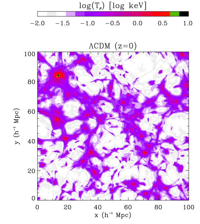
FIG. 1.: Density-weighted temperature for the $\Lambda$CDM simulation at $z=0$. The temperature map was derived by projecting through one face of the box.

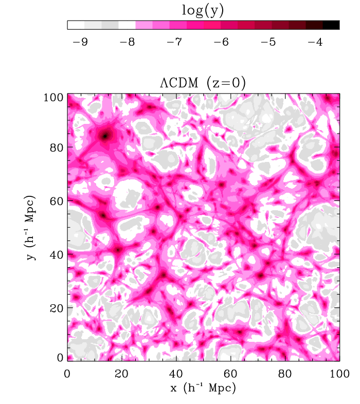
FIG. 2.: Comptonization-parameter map for the $\Lambda$CDM simulation at $z=0$.

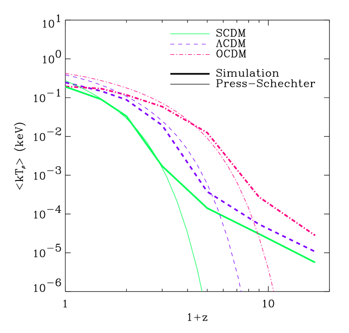
FIG. 3.: Temperature history of the gas. For each model, the density weighted temperature $T_{\rho}$ is shown for the simulations and for the Press-Schechter prediction.

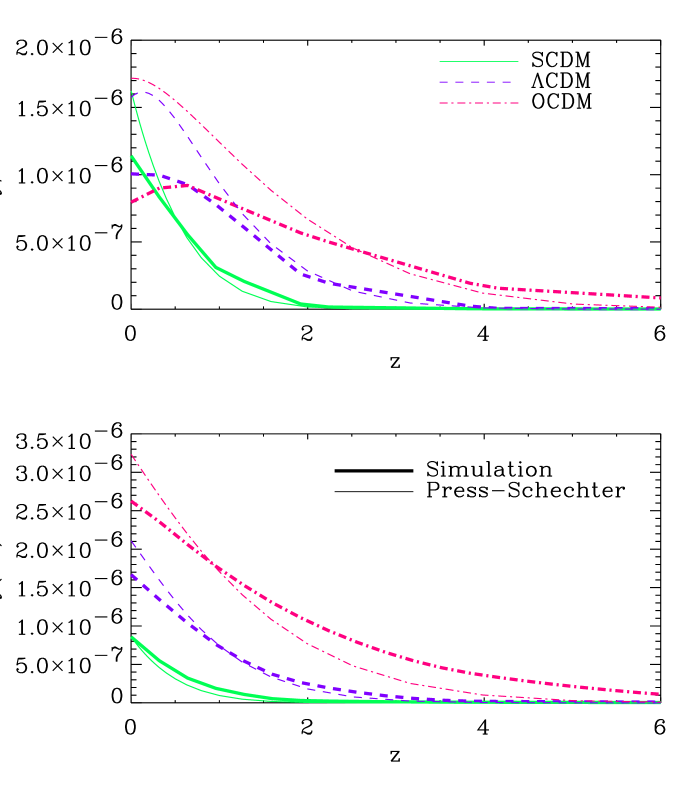
FIG. 4.: Differential and cumulative $y$-parameter versus redshift, for each simulation. The cummulative $y$-parameter predicted from the Press-Schechter formalism is shown as the thin lines.

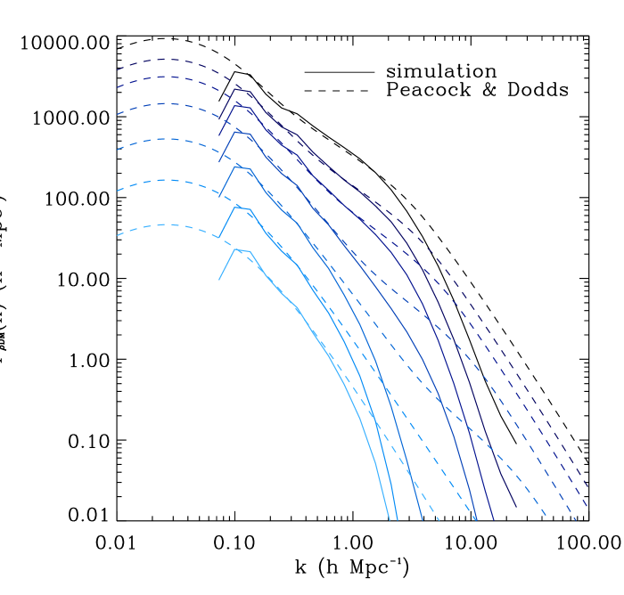
FIG. 5.: Power Spectrum of the DM density for the $\Lambda$CDM simulation. The power spectrum from the simulation (solid lines) is compared to that from the Peacock & Dodds (1996) fitting formula (dashed lines). The spectra, from top to bottom, correspond to $z$=0, 0.5, 1, 2, 4, 8, and 16.

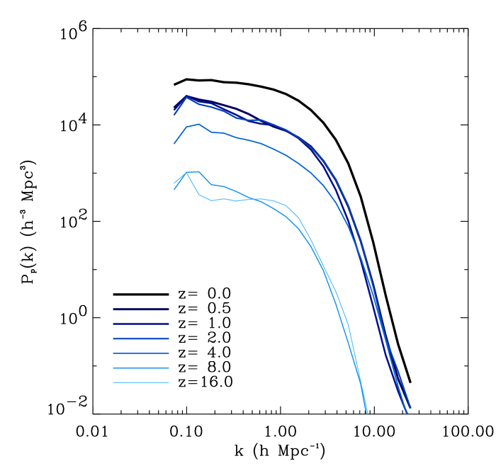
FIG. 6.: Power spectrum of the pressure fluctuations for the $\Lambda$CDM model.

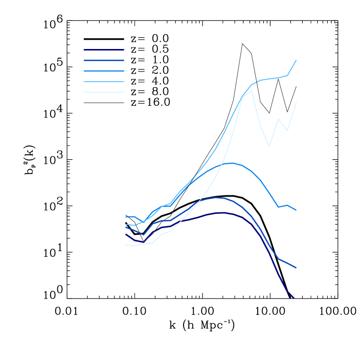
FIG. 7.: Bias of the pressure $b_{p}(k,z)$ for the $\Lambda$CDM model.

FIG. 8.: Power spectrum of the SZ effect for each model in the RJ regime, as derived from the simulations. The approximate range of confidence ($200<l<2000$) is highlighted by thicker lines. The power spectra outside of this range should be taken as lower limits. For comparison, the primary CMB power spectrum is shown for the $\Lambda$CDM model. The $1\sigma$ uncertainty for the 94GHz map channel is shown, for a band average of $\Delta l=10$. The power spectrum for the residual discrete sources ($>2$Jy) for the 94 GHz MAP channel is also shown.

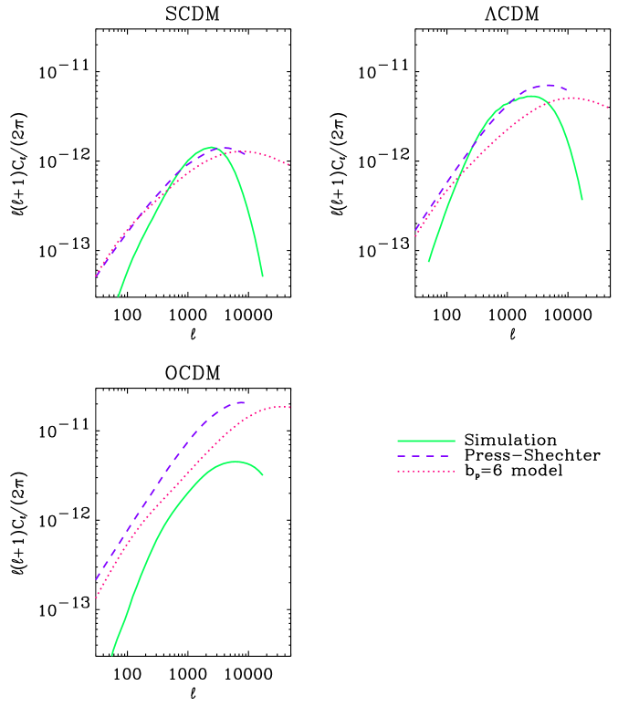
FIG. 9.: Angular power spectrum of the SZ effect from each method: simulations, the PS formalism, and the constant bias model (with $b_{p}=6$). These results are shown for the RJ regime, for each cosmological models.

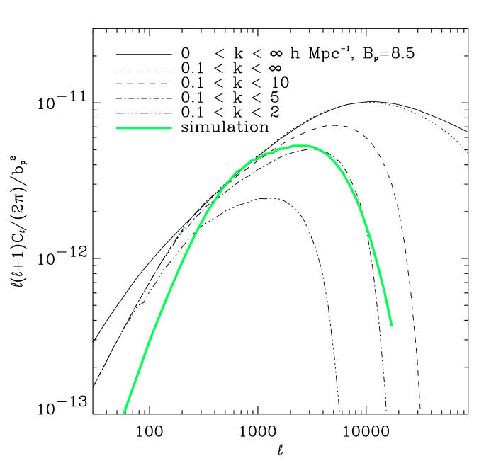
FIG. 10.: Effect of resolution and finite box size on the SZ power spectrum. The $\Lambda$CDM power spectrum is shown for the constant bias model (with $b_{p}=8.5$), for several restricted ranges of $k$ values for the pressure power spectrum $P_{p}(k,z)$. While the finite box size ($0.1<k<\infty\ h$ Mpc^-1) does not have much effect, the finite resolution of the simulations ($0.1<k<2,5,10\ h$ Mpc^-1) reduce the full power spectrum ($0<k<\infty$) considerably outside of the approximate range $200<l<2000$.

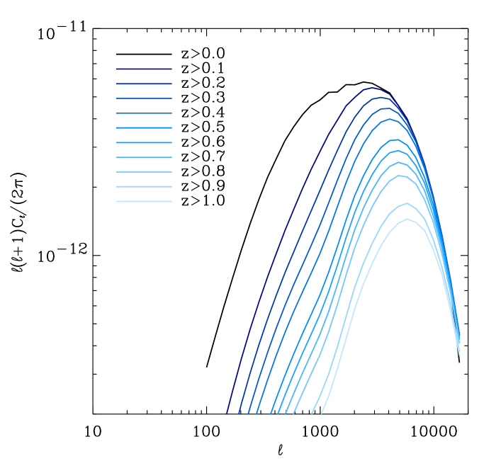
FIG. 11.: Dependence of SZ power spectrum on redshift. For the $\Lambda$CDM model, the contribution to the SZ power spectrum up to a given redshift is shown.

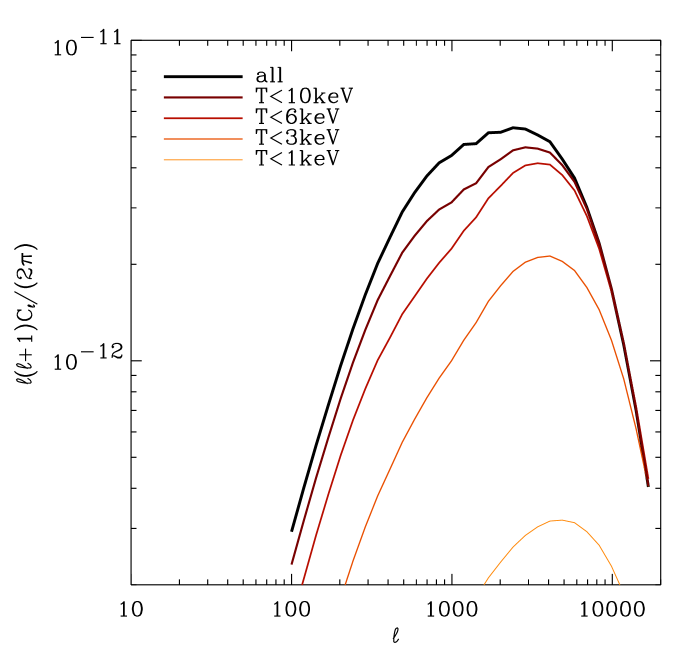
FIG. 12.: SZ power spectrum as a function of temperature for the $\Lambda$CDM model. The SZ power spectrum was calculated after removing regions with temperatures above the specified cutoff.