Star Formation and Structure Formation at
Abstract
The advent of 8m-class telescopes has made galaxies at relatively easy to detect and study. This is a brief and incomplete review of some of the recent results to emerge from surveys at these redshifts. After describing different strategies for finding galaxies at , and the differences (and similarities) in the resulting galaxy samples, I summarize what is known about the spatial clustering of star-forming galaxies at . Optically selected galaxies are the main focus of this review, but in the final section I discuss the connection between optical and sub-mm samples, and argue that the majority of the m background may have been produced by known optically selected populations at high redshift. Among the new results presented are the dust-corrected luminosity function of Lyman-break galaxies at , the estimated contribution to the m background from optically selected galaxies at , revised estimates of the spatial clustering strength of Lyman-break galaxies at , and an estimate of the clustering strength of star-forming galaxies at derived from a new spectroscopic sample of galaxies with , .
Palomar Observatory, Caltech 105–24, Pasadena, CA 91125
1. Introduction
An ambitious goal in cosmology is to understand how the universe evolved from its presumed beginning in the Big Bang to the familiar collection of stars and galaxies that we observe around us today. The last decade has seen tremendous progress in understanding the large role that gravitational instability almost certainly played. Although we still do not have complete analytic understanding, reasonable analytic approximations for the growth of gravitationally driven perturbations are now known, and sophisticated N-body simulators and simulations are freely available for obtaining more precise or detailed information. Remarkable progress has also been made in observationally constraining the initial conditions that are required as input to the simulations or approximations. The available data appear largely consistent with the idea that primordial fluctuations were Gaussian (e.g. Bromley & Tegmark 1999) with a power-spectrum similar to that of an adiabatic CDM model over orders of magnitude in spatial scale (e.g. numerous recent results from observations of the cosmic microwave background, reviewed most recently by Scott 2000; White, Efstathiou, & Frenk 1993; Croft et al. 1999).
But gravitational instability is only half—the easy half!—of the story. It alone cannot tell us how or when the stars that populate the universe today were formed. Presumably stars began to form within overdensities in the matter distribution as these overdensities slowly evolved from small ripples in the initial conditions into the large collapsed objects of today, but modeling this has proved tremendously difficult. We cannot easily model the formation of a single star (see Abel’s contribution to these proceedings), let alone the ten billion stars in a typical galaxy. Even the most sophisticated theoretical treatments of galaxy formation rely on simplified “recipes” for associating the formation of stars with the gravitationally driven growth of perturbations in the underlying matter distribution. The adopted recipes for star formation, although physically plausible, are by far the most uncertain component in theoretical treatments of galaxy formation. We will need to check them through observations of star-forming galaxies at high-redshift before we can be confident that our understanding of galaxy formation is reasonably correct. These observations, and their implications, are the subject of my talk.
2. Finding Galaxies at
In the past 5 years several techniques have been shown effective for finding galaxies at . I don’t have space to list them all; a partial list would include deep optical magnitude limited surveys (e.g. Cohen’s contribution to these proceedings), narrow band surveys (e.g. Hu, Cowie, & McMahon 1998), targeted surveys around known AGN at (e.g. Hall & Green 1998, Djorgovski et al. 1999), m surveys (e.g. Ivison et al. 2000), and color-selected surveys (e.g. Steidel et al. 1999, Adelberger et al. 2000). Different selection techniques have different advantages and are optimized for answering different questions. Color-selected surveys, which detect numerous galaxies over large and (hopefully) representative volumes, are especially well suited for studying large scale structure at high redshift. They will be the main focus of this review.
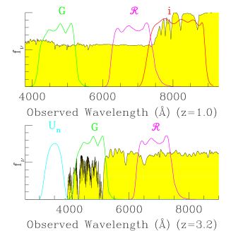
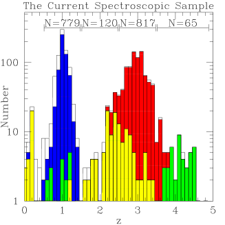
In color-selected surveys, spectra are obtained only for objects with broad-band colors indicating that they are likely to lie at a given redshift. The left panel of Figure 1 illustrates why galaxies at certain redshifts have distinctive broad-band colors. The right panel shows spectroscopic redshifts for galaxies satisfying various simple color selection criteria, demonstrating that color selection is a reasonably effective way of finding galaxies at a range of redshifts . At these galaxies were selected by exploiting the Balmer-break (Adelberger et al. 2000), at and by exploiting the Lyman-break (Steidel et al. 1999), and at by an approach similar to the “UV drop in” technique described by Roukema in these proceedings. The data in Figure 1 represent only our own efforts; many more galaxies at similar (and higher) redshifts have been found by other groups with a variety of techniques.
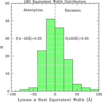
Although different strategies for finding galaxies at result in samples weighted towards different types of objects, there is nevertheless significant overlap between the galaxy populations that are found. The left panel of Figure 2, showing the Ly- equivalent width distribution of color-selected Lyman-break galaxies at , illustrates the point. About 20% of Lyman-break galaxies have equivalent widths large enough to be detected in standard narrow-band searches for high redshift galaxies. At fixed continuum luminosity, narrow-band searches detect only the fraction of galaxies with the largest equivalent widths, and at fixed equivalent width, color-selected surveys detect only the fraction of galaxies with the brightest continua; but the galaxies detected with these techniques appear to belong to the same underlying population. Similarly, although the Balmer-break selection criteria of Adelberger et al. (2000) are designed to select optically bright star-forming galaxies at , a substantial fraction of these galaxies (the limited available data suggests 1 in , or per square arcmin to ) have the red optical-to-infrared colors that are often thought to be characteristic of extremely dusty or old galaxies at this redshift. Many of the same galaxies will therefore be found both by surveys for old or dusty galaxies at that exploit their expected large optical-to-infrared colors and by surveys for star-forming galaxies at that exploit the Balmer break. Finally, there is even some overlap between far-UV selected samples and far-IR selected samples of galaxies at high redshift, though these two selection strategies might have been expected a priori to find completely different populations of objects. For example, the two mJy sources robustly identified with star-forming galaxies (as opposed to AGN) at , SMMJ14011+0252 at (Ivison et al. 2000) and West-MMD11 at (Chapman et al. 2000), have the relatively blue far-UV colors observed in optically selected galaxies at similar redshifts; they are typical, aside from their unusually bright far-UV luminosities, of the kind of galaxies found in optical surveys.
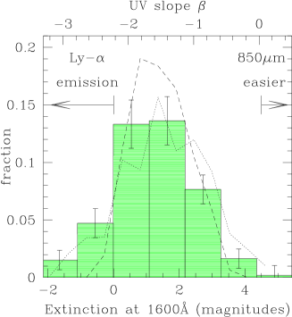
The relationship between sub-mm selected and UV-selected high-redshift populations can be partially understood with plots like the right panel of Figure 2, which shows the inferred distribution of dust opacities among optically selected galaxies at (Adelberger et al. 2000). These dust opacities were estimated with a relationship between and far-UV spectral slope that is obeyed by starburst galaxies in the local universe (e.g. Meurer, Heckman, & Calzetti 1999). It is not known if high-redshift galaxies obey this relationship; see §4 below. The majority of galaxies at this redshift appear to have middling dust opacities and are therefore far easier to detect in the optical than at m, but some galaxies, even in optical surveys, are so dusty that they would have been easier to detect with sub-mm rather than optical imaging. Although relatively dust-free galaxies appear to dominate high-redshift populations by number, it is unclear if they dominate by star-formation rate: dusty galaxies tend to have much larger star-formation rates and this compensates, to some unknown but probably large extent, for their smaller numbers. I will discuss this further in §4.
3. Spatial Clustering in High-Redshift Samples
The large samples of star-forming galaxies at produced by color-selected surveys allow one to begin to try to fit star-forming galaxies into the larger context of structure formation in the universe. The most obvious way to make a connection between the observed galaxies and perturbation in the underlying distribution of matter is to attempt to estimate the masses associated with individual galaxies by observing their velocity dispersions. Unfortunately this approach is surprisingly difficult. To begin with, it is hard to measure velocity widths for high-redshift galaxies. The [OII], H, and [OIII] nebular emission lines of galaxies at , for example, are redshifted into the bright sky of the near-IR, and as a result perhaps only 2–3 velocity widths can be measured per night even with an 8m-class telescope. A more serious problem is interpreting the velocity widths that have been measured. The limited available data suggest that most Lyman-break galaxies at have nebular line widths corresponding to 70–80 km/s, for example (Pettini et al. 1998, 2000). These velocity dispersions are far smaller than the circular velocities that were expected for Lyman-break galaxies on a number of other grounds (e.g. Baugh et al. 1999; Mo, Mao, & White 1999) and this has led some to suggest that Lyman-break galaxies are low mass “satellite galaxies” undergoing mergers (e.g. Somerville’s and Kolatt’s contributions to these proceedings). But because the baryons in these galaxies presumably cooled and collapsed farther than the dark matter before stars began to form, their nebular line widths are expected to be significantly smaller than the full circular velocity of the dark matter potential. The exact size of the difference is not easy to calculate. Analytic attempts at the calculation (e.g. Mo, Mao, & White 1999) rely on a large number of simplifying assumptions, but the real situation may not be so simple: Lehnert & Heckman (1996) and Kobulnicky & Gebhardt (2000) have presented evidence for a complicated relationship between nebular line widths and circular velocities in the local universe among late-type and starburst galaxies that are presumably the closest analogs to detected high-redshift galaxies.
The spatial distribution of high redshift galaxies provides an alternate way of making a connection between star-forming galaxies and perturbations in the underlying distribution of dark matter. For a given cosmogony the spatial distribution of matter at any redshift is straightforward to calculate with simulations or analytic approximations. Once large numbers of star-forming galaxies have been detected near a single redshift we can therefore ask, for example, what kinds of collapsed objects in the expected distribution of mass at that redshift have the same spatial distribution as the observed galaxies. In this way we can attempt to place star-forming galaxies in the larger context of structure formation. Observational constraints on the spatial clustering of galaxies at will be the main subject of this section, starting at and moving later to .
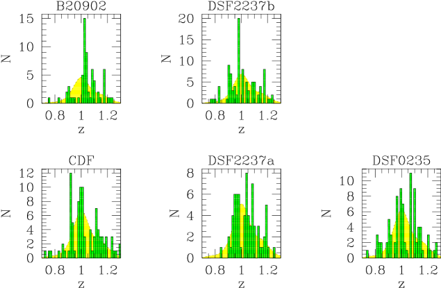
Attempts to measure clustering strength for galaxies at have been carried out by Carlberg et al., Le Fevre et al., and Cohen et al.; their results are reviewed in Cohen’s contribution to these proceedings. Here I will focus instead on previously unpublished results from a survey of star-forming galaxies at (Adelberger et al. 2000). This sample consists of several thousand photometric candidates with ; to date redshifts have been obtained for of them. The mean redshift of the spectroscopically observed candidates is and the standard deviation is . We currently have uniform spatial spectroscopic sampling in four and one square fields. Roughly 100 redshifts have been obtained in each (Figure 3).
In the four fields, the variance of galaxy counts in cubes of comoving side length Mpc (, ), estimated as described in Adelberger et al. 1998 from the data in Figure 3, is . For a power-law spatial correlation function of the form —which is consistent with the angular clustering of these galaxies—this variance corresponds to a comoving correlation length of Mpc, or a variance of galaxy counts in spheres with radius Mpc of . The Mpc variance is similar to the expected variance of mass at in spheres of the same size, estimated by evolving back to with linear theory the value of determined at from the abundance of galaxy clusters (e.g. Eke, Cole, & Frenk 1996). Balmer-break galaxies are evidently fairly unbiased tracers of mass fluctuations at (for the , cosmology assumed throughout). Evolving their clustering strength forward to with the linear prescription of Tegmark & Peebles (1998) suggests that these galaxies are likely the progenitors of galaxies with in the local universe, i.e. relatively normal galaxies. This result could perhaps have been anticipated from the comoving abundance of Balmer-break galaxies, which, at to , is similar to that of galaxies in the local universe.
The increase in clustering strength from galaxies in our sample at to galaxies at therefore appears to be relatively easy to understand; it is almost exactly what one might have expected gravitational instability to have produced acting on a population of formed objects. Remarkably the same is not true at higher redshifts. Rather than decreasing further, at redshifts the observed clustering strength of detected star-forming galaxies begins to rise.
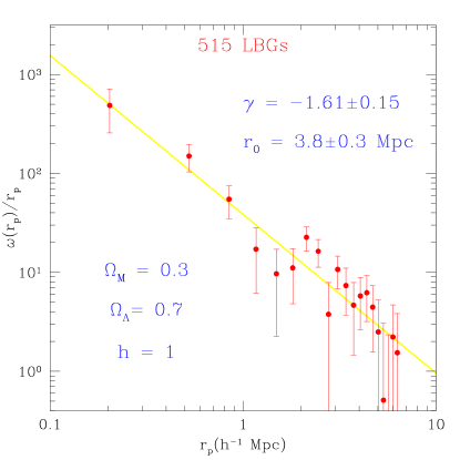
Hints that star-forming galaxies at might be strongly clustered were first provided by targeted surveys of small and carefully selected volumes, often around known AGN (e.g. Giavalisco, Steidel, & Szalay 1994; Le Fevre et al. 1996; Francis et al. 1997; see also later work by Campos et al. 1999 and Djorgovski et al. 1999). Further evidence came subsequently from the color-selected survey of Lyman-break galaxies at (e.g. Steidel et al. 1998). Figure 4 shows the projected correlation function (e.g. Davis & Peebles 1983) of galaxies in this sample. The implied correlation length, neglecting systematic errors, is Mpc comoving (, ). A similar estimate of the correlation length follows from the relative variance of Lyman-break galaxy counts in cubes of comoving side-length Mpc, (Adelberger et al. 2000; this value supersedes our previous estimate, which was based on a smaller data set).
Gravitational instability acting on a population of galaxies that had comoving Mpc at would not produce a population with comoving Mpc (similar to the observed of Balmer-break galaxies) at or a population with comoving Mpc (similar to normal local galaxies) at . This can be shown in a crude way by first assuming that the correlation function of Lyman-break galaxies selected at would maintain a constant slope of at lower redshifts, and then using the linear approximation of Tegmark & Peebles (1998) to evolve the observed clustering of Lyman-break galaxies at to lower redshifts. Limited space does not allow a more careful analysis or the consideration of cosmological models besides , , although both would affect our conclusions somewhat. In this simplified analysis, we would expect former Lyman-break galaxies to have comoving Mpc at and comoving Mpc at .
These correlation lengths are significantly larger than those of Balmer-break galaxies at and of normal galaxies at , implying that Lyman-break galaxies are unlikely to be the progenitors of either population. What are they instead? Why is their spatial clustering so much stronger than we might naively have expected? A clue is provided by their number density, (, ) to , which is about 5 times lower than the number density of normal galaxies in the local universe or of Balmer-break galaxies with in our sample. Perhaps the relatively rare Lyman-break galaxies are not progenitors of typical galaxies at but instead are special in some way. One way in which they are special is that they are the UV-brightest galaxies (and therefore presumably the most rapidly star-forming galaxies) at . Semi-analytic calculations (e.g. Baugh et al. 1998, Kauffmann et al. 1999) suggest that the most rapidly star-forming galaxies at high redshift will reside within the most massive collapsed objects, rather than within typical collapsed objects, and so perhaps we can understand the clustering of Lyman-break galaxies by trying to associate them with massive collapsed objects at instead of with galaxy populations at lower redshift.
In a classic paper, Kaiser (1984) showed that in hierarchical models the most massive collapsed objects at any redshift are more strongly clustered than the distribution of matter as a whole. A formalism for estimating the clustering strength of collapsed objects as a function of mass was subsequently developed by many authors; see (e.g.) Mo & White (1996). Remarkably the observed clustering of Lyman-break galaxies is indistinguishable (as far as we can tell—see Wechsler’s contribution to these proceedings) from the predicted clustering of the most massive collapsed objects at down to a similar abundance (e.g. Adelberger et al. 1998). This result suggests that there may indeed be a simple relationship between mass and star-formation rate in high redshift galaxies, as many semi-analytic models predicted (e.g. Baugh et al. 1998).
If the mass of a galaxy plays a dominant role in determining its star formation rate, then we might expect the star-formation rate distribution of galaxies to be related in a simple way to the distribution of masses of collapsed objects at . As a crude guess at the star-formation rate associated with a collapsed “halo,” we can take the mass cooling rate in the halo for large masses and the mass cooling rate times a number proportional to for small masses where supernova feedback is important (e.g. White & Frenk 1991). In this approximation, for cooling dominated by Bremsstrahlung, we would expect for large and for small . Figure 5 shows the slopes of our simplistic “theoretical” SFR distribution in these two limits. At each abundance the slope of the mass function was estimated with the Press-Schechter (1974) approximation for an , , , , cosmogony; changing the values of any of these parameters would change the mass function slope somewhat. Also shown in Figure 5 is the observed “dust-corrected” luminosity function of these galaxies, estimated using the – correlation of Meurer et al. (1999) as described in Adelberger & Steidel (2000). The observed slopes agree reasonably well with our naive expectations, but the star-formation rates at any abundance are unexpectedly high, many times larger than the expected cooling rate for halos of similar abundance. (Standard formulae can be used to derive star-formation rates from the far-UV luminosities shown in Figure 5; see, e.g., Madau, Pozzetti, & Dickinson 1998.) This has been taken as evidence that the star formation in Lyman-break galaxies is fueled not by quiescent cooling but instead by the rapid cooling that would accompany a merger of two smaller galaxies (e.g. Somerville’s and Kolatt’s contributions to these proceedings). Many uncertain steps lie behind the conclusion that the star formation rates in Lyman-break galaxies far exceed their quiescent cooling rates, however. The star-formation rates of Lyman-break galaxies could be considerably lower than is usually deduced, for example, if we are wrong about the shape of the IMF, about the magnitude of the required dust corrections, or even about the value of various cosmological parameters, while the cooling rates in Lyman-break galaxies could be significantly higher than usual estimates if we are wrong about the baryon fraction, the metallicity, or the spatial distribution of the gas or dark matter in these galaxies. It would be tremendously interesting if the star formation rates of Lyman-break galaxies really were far higher than their quiescent cooling rates, but I do not think this has been conclusively shown.
In any case I will assume for now that Lyman-break galaxies are strongly clustered because they reside within rare and massive collapsed objects at , and return to the question of how they might be related to the Balmer-break galaxies observed at . The calculation above showed that Lyman-break galaxies with cannot be the progenitors of Balmer-break galaxies with , and this was hardly surprising since the abundance of the Lyman-break galaxies is so much lower. But suppose we had significantly deeper photometry, so that we could detect fainter Lyman-break galaxies and reach an abundance similar to that of Balmer-break galaxies at . Could this deeper population of Lyman-break galaxies evolve into a population like the Balmer-break galaxies by ? If halo mass and star formation rate are related in the simple way described above, then the deep Lyman-break population would be somewhat less strongly clustered that the current population, helping to remove the inconsistency between the observed of Balmer-break galaxies and the expected of Lyman-break galaxy descendants. A deep Lyman-break population, with abundance times that of the sample, has in fact been detected in the HDF, and its correlation length (which cannot be measured very accurately because of the HDF’s small size) appears smaller than that of the brighter ground-based population (Giavalisco et al. 2000); but it looks like this effect is not strong enough to remove the inconsistency in clustering strength for Lyman-break galaxy descendants and Balmer-break galaxies at . We are left with the result that galaxies selected by the Balmer-break technique at are probably not (for the most part) the descendants of those detected with the Lyman-break technique at . Because Balmer-break galaxies appear to be representative of typical star-forming galaxies at , the simplest interpretation is that Lyman-break galaxies have largely stopped forming stars by —are they perhaps instead passively evolving into the elliptical galaxies observed at lower redshifts?
In principle this sort of argument could provide a very stringent constraint on the star-formation rates of Lyman-break galaxy descendants at , since (for , ) galaxies with as little as /yr of star formation would have bright enough UV continua (in the absence of dust obscuration) to be included in our Balmer-break sample. But I am still not convinced that the argument is completely robust; firmly establishing that former Lyman-break galaxies are not significantly forming stars at will require a much better understanding than is currently available of the clustering of fainter and more numerous Lyman-break galaxies at and of what kinds of star-forming objects might not satisfy our “Balmer-break” selection criteria at .
4. Dust
A full observational understanding of star formation at high redshift can only be achieved if we are able to detect most of the star formation in representative portions of the high redshift universe. But how can we be sure that our surveys are not missing a large fraction of the star formation at high redshift? The sad answer is that we can’t. There are too many ways that star formation could be hidden from our surveys for us ever to be sure that we have detected most of it. Surveys cannot detect the star formation that occurs in objects below their flux and surface brightness limits, for example, and they cannot directly detect the formation of the low mass stars that (at least in the local universe) dominate the total stellar mass. At best we can aim for a reasonably complete census of the formation of massive stars that occurs in objects above our flux and surface brightness limits. If these limits are deep enough, and if the high-redshift IMF is similar enough in all environments to what we have assumed, then this sort of sample can serve as an acceptable proxy for a true census of all star formation at high redshift.
What is the best way to produce a reasonably complete survey of massive star formation? Massive stars emit most of their luminosity in the UV, and so naively we might choose a deep UV-selected survey. It has become clear in recent years, however, that most of the UV photons emitted by stars in rapidly star-forming galaxies are promptly absorbed by dust, and as a result most of the luminosity produced by massive stars tends to emerge from these galaxies in the far-IR where dust radiates. This is true in the local universe for a broad range of rapidly star-forming galaxies, from the famous class of “Ultra Luminous Infrared Galaxies” (ULIRGs, galaxies with ) to the much fainter UV-selected starbursts contained in the IUE Atlas (e.g. Meurer et al. 1999); and the recent detection of a large extragalactic far-IR background (e.g. Fixsen et al. 1998) suggests that it is likely to have been true at high redshifts as well.
Two implications follow. The first is that far-IR luminosities probably provide a better measurement of rapidly star-forming galaxies’ star-formation rates than do UV luminosities. The second is that even very rapidly star-forming galaxies may not be detected in a UV selected survey if they are sufficiently dusty. Far-IR/sub-mm selected surveys should therefore in principle provide a much better census of massive star formation at any redshift than UV selected surveys. m surveys are likely to provide an especially good census at , because favorable -corrections make a galaxy that is forming stars at a given rate appear almost equally bright at m for any redshift in this range (see Hughes’ contribution to these proceedings), and consequently a flux-limited sample at m is nearly equivalent to a star-formation limited sample at .
This is exactly the kind of sample that detailed attempts to understand star formation at high redshift require. So why then was most of this review devoted to UV-selected high redshift samples rather than the apparently superior m samples? The reason is that m observations are comparatively difficult. The deepest m image taken with SCUBA (the current state-of-the-art sub-mm bolometer array) reached a depth of 2mJy in a square arcminute region of the sky, for example, and five sources were detected (Hughes et al. 1998). In contrast a modern instrument on a 4m-class optical telescope can easily obtain photometry to a depth of Jy over a square arcminute region, detecting thousands of galaxies at . Even though optical surveys do not select star-forming galaxies in the optimal way, most of what we know about galaxies at high redshift comes (and will continue to come for many years) from these surveys. The question—probably the most important question for those interested in high-redshift galaxy formation—is whether the large and detailed view of the high redshift universe provided by UV selected surveys is reasonably complete.
This is equivalent to asking whether the galaxies responsible for producing the m extragalactic background are bright enough in the rest-frame UV to be included in current optical surveys. If they are not, then optically selected surveys will not be able to teach us much of value about high-redshift star formation despite the wealth of information they contain.
The straightforward way to constrain the UV luminosities of the objects that produce the m background is to observe the UV luminosities of known m sources. This is difficult in practice, however, because relatively few m sources have been detected and each has a significant positional uncertainty due to SCUBA’s large diffraction disk. Often several optical sources lie within a sub-mm error box, and a great deal of effort is required to determine which one is the true optical counterpart (e.g. Ivison et al. 2000). Moreover only about 30% of the m background can be resolved into discrete sources with current technology, and so optical observations of detected m sources cannot conclusively tell us about the optical luminosities of the galaxies responsible for producing most of the m background.
An alternate approach, taken by Adelberger & Steidel (2000), is to estimate the contribution to the m background from known optically selected populations at high redshift and compare this expected background to the observed background to see if there is significant shortfall.
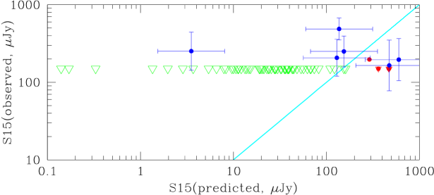
Meurer et al. (1999) have shown that the far-IR luminosities of UV-selected starbursts in the local universe can be estimated to within a factor of from the starbursts’ UV luminosities and spectral slopes . Their /far-IR relationship was the foundation of our calculation. It is not known if high-redshift galaxies obey this relationship. Chapman et al. (2000) presented evidence that the m fluxes of Lyman-break galaxies may be somewhat lower than the relationship would suggest, but the evidence is very marginal when the uncertainties in Lyman-break galaxies’ predicted m fluxes are taken into proper account. Adelberger & Steidel (2000) have checked in a number of other ways whether star-forming galaxies obey the relationship. Figure 6, showing the predicted and observed m fluxes of Balmer-break galaxies in the sample described above, is an example. The predicted fluxes in Figure 6 assume that these galaxies will follow both the /far-IR correlation of Meurer et al. (1999) and the correlation between 6–9m luminosity and far-IR luminosity observed in the (star-forming) ULIRG sample of Genzel et al. (1998) and Rigopoulou et al. (2000). The m data are from the ISO LW3 observations of Flores et al. (1999). A large fraction of objects with predicted fluxes below the detection limit were not detected, and a large fraction of objects with predicted fluxes above the detection limit were detected. This plot therefore provides some support for the notion that Balmer-break galaxies at obey the /far-IR relationship.
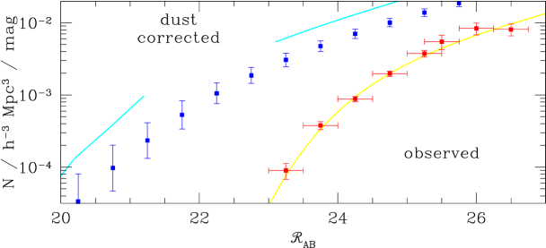
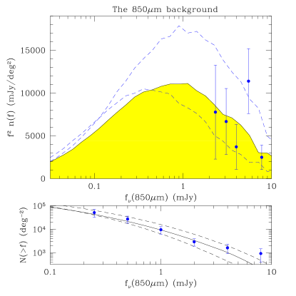
If we assume that all optically selected galaxies at obey this relationship, then we can make crude estimate of their total contribution to the m background. In this calculation I will assume further that the comoving star formation density in optically selected populations is constant for (e.g. Steidel et al. 1999), that the dust SEDs of optically selected galaxies at are similar to those of starbursts and ULIRGs in the local universe, and that the (unknown) luminosity and distributions of optically selected galaxies at are similar to those measured for Lyman-break galaxies at . (See Adelberger & Steidel 2000 for a more complete discussion.) Under these assumptions optically selected populations at would be expected to produce m number counts and background that are surprisingly close to the observations (Figure 7).
Although the overall agreement is good, within the substantial uncertainties, there appear to be significant differences at the brightest m fluxes. Optically selected galaxies cannot easily (it seems) account for the large number of observed sources with mJy, and indeed Barger, Cowie, & Richards (1999) have shown that these sources tend to have extremely faint optical counterparts. It is possible that these bright sources are associated with AGN, rather than the star-forming galaxies we have included in our calculation, but in any case it appears that the bulk of the m background could have been produced by known optically selected populations at high redshift. This claim rests on a large number of assumptions that could easily be wrong, but I am willing to bet $100 that when ALMA finally resolves the background we will discover that most of it is produced by galaxy populations already detected and studied in the rest-frame UV. Any takers?
Acknowledgments.
I would like to thank the organizers for support and for considerable patience. Special thanks are due to my collaborators C. Steidel, M. Dickinson, M. Giavalisco, M. Pettini, and A. Shapley for their contributions to this work. Super special thanks go to C.S. for his comments on an earlier draft.
References
Adelberger, K. L. et al. 1998, ApJ, 505, 18
Adelberger, K. L. & Steidel, C. C. 2000, ApJ, submitted
Adelberger, K. L. et al. 2000, AJ, in preparation
Barger, A. J., Cowie, L. L., & Sanders, D. B. 1999, ApJL, 518, 5
Barger, A. J., Cowie, L. L., & Richards, E. A. 1999, in ASP Conf. Proc., Photometric Redshifts and the Detection of High Redshift Galaxies, ed. R. Weymann et al. (San Francisco: ASP)
Baugh, C. M., Cole, S., Frenk, C. S., & Lacey, C. G. 1998, ApJ, 498, 504
Blain, A. W., Kneib, J.-P., Ivison, R. J., & Smail, I. 1999, ApJL, 512, L87
Bromley, B. C. & Tegmark, M. 1999, ApJL, 524, L79
Campos, A. et al. 1999, ApJL, 511, L1
Chapman, S. et al. 2000, MNRAS, submitted
Croft, R. A. C., Weinberg, D. H., Pettini, M., Hernquist, L., & Katz, N. 1999, ApJ, 520, 1
Davis, M. & Peebles, P. J. E. 1983, ApJ, 267, 465
Djorgovski, S. J. et al. 1999, in ASP Conf. Proc., Photometric Redshifts and the Detection of High Redshift Galaxies, ed. R. Weymann et al. (San Francisco: ASP)
Eke, V. R., Cole, S., & Frenk, C. S. 1996, MNRAS, 282, 263
Fixsen, D. J. et al. 1998, ApJ, 508, 123
Flores, H. et al. 1999, ApJ, 517, 148
Francis, P. J., Woodgate, B. E., & Danks, A. C. 1997, ApJL, 482, 25
Genzel, R. et al. 1998, ApJ, 498, 579
Giavalisco, M., Steidel, C. C., & Szalay, A. S. 1994, ApJL, 425, L5
Giavalisco, M. et al. 2000, ApJ, in preparation
Hall, P. B. & Green, R. F. 1998, ApJ, 507, 558
Hu, E. M., Cowie, L. L., & McMahon, R. G. 1998, ApJL, 502, L99
Hughes, D. H. et al. 1998, Nature, 394, 241
Ivison, R. et al. 2000, MNRAS, in press
Kaiser, N. 1984, ApJL, 284, L9
Kauffmann, G., Colberg, J. M., Diafero, A., & White, S. D. M. 1999, MNRAS, 307, 529
Kobulnicky, H. A. & Gebhardt, K. 2000, AJ, in press
Le Fevre, O., Deltorn, J. M., Crampton, D., & Dickinson, M. 1997, ApJL, 471, 11
Lehnert, M. D. & Heckman, T. M. 1996, ApJ, 472, 546
Madau, P., Pozzetti, L., & Dickinson, M. 1998, ApJ, 498, 106
Mo, H. J., & White, S. D. M., 1996, MNRAS, 282, 347
Mo, H. J., Mao, S., & White, S. D. M. 1999, MNRAS, 304, 175
Pettini, M. et al., 1998, ApJ, 508, 539
Pettini, M. et al., 2000, ApJ, in preparation
Press, W. H. & Schechter, P. 1974, ApJ, 187, 425
Rigopoulou, D. et al. 1999, AJ, in press
Scott, D. 2000, in ASP Conf. Proc., Cosmic Flows, ed. S. Courteau et al. (San Francisco: ASP)
Steidel, C. C. et al, 1998, ApJ, 492, 428
Steidel, C. C. et al. 1999, ApJ, 519, 1
Steidel, C. C. et al. 2000, ApJ, in press
Tegmark, M. & Peebles, P. J. E., 1998, ApJL, 500, L79
White, S. D. M., Efstathiou, G. & Frenk, C. S. 1993, MNRAS, 262, 1023
White, S. D. M. & Frenk, C. S. 1991, ApJ, 379, 25