The Eddington Luminosity Phase
in Quasars: Duration and Implications

Abstract

Non-steady and eruptive phenomena in quasars are thought to be associated with the Eddington or super-Eddington luminous stage. Although there is no lack in hypotheses about the total duration of such a stage, the latter remains essentially unknown. We calculate the duration of quasar luminous phase in dependence upon the initial mass of a newborn massive black hole (MBH) by comparing the observed luminosity- and redshift distributions of quasars with mass distribution of the central MBHs in normal galactic nuclei. It is assumed that, at the quasar stage, each MBH goes through a single (or recurrent) phase(s) of accretion with, or close to, the Eddington luminosity. The mass distributions of quasars is found to be connected with that of MBHs residing in normal galaxies by a one-to-one corrrespondence through the entire mass range of the inferred MBHs if the accretion efficiency of mass-to-energy transformation $\eta\sim 0.1$.

Introduction

An approximate relationship $M_{h}\simeq(0.003-.006)M_{b}$ between the central MBH mass, $M_{h}$, and that of the galactic bulge, $M_{b}$, has been established for a few dozen of galaxies, both nearby and more distant ones 0003 ,0006 . A relationship between absolute magnitudes of quasars and their host galaxies found in Bahc is reduced to the MBH to bulge mass relation in galaxies provided that oz98 : (i) the central MBH shines at or near to the Eddington luminosity and (ii) the host galaxy undergoes through a starburst episode. This correlation, coupled with the known luminosity function of galaxies, can serve to obtain S98 the MBH mass distribution $\phi_{1}(M_{h})dM_{h}$. The history of matter accretion onto a central MBH thought to serve as a source of quasar activity is linked to the present observable properties of each individual quasar, such as its luminosity, variability, and emission spectrum. If the bolometric luminosity of a quasar comprises a fraction $\lambda$ of the Eddington luminosity, i.e. $\lambda=L/L_{E}$, $L_{E}=4\pi GM_{h}m_{p}c/\sigma_{T}$, the underlying accretion is accompanied by an exponential growth of the MBH mass with the characteristic time $t_{E}=4.5\cdot 10^{8}\eta/\lambda\mbox{~{}yrs}$, where $\eta$ is the accretion efficiency of mass-to-energy transformation. The crucial problem is the duration, $t_{q}$, of such a nearly Eddington accretion phase. Usually an effective $t_{q}$, the same for the entire black hole mass range $M_{h}\sim 10^{6}-10^{10}M_{\odot}$, is calculated by comparing the global number density of normal galaxies and quasars and is found to be $t_{q}=10^{6}-5\cdot 10^{8}$ years in HNR97 . Meanwhile the recent data on mass distribution of MBHs in galaxies provide an opportunity to solve this problem in a more detailed way, viz., to calculate the dependence of $t_{q}$ upon $M_{h}$, which is the major aim of this paper. We shall explore whether the distribution functions of quasars and MBHs in normal galaxies are consistent with each other, and we will do this locally in the vicinity of each mass.

The Eddington Luminosity Phase

It would be reasonable to assume that the duration of the Eddington phase $t_{q}$ depends on the initial mass of a newborn MBH or, in other words, on the initial luminosity, $L_{i}$, of the quasar: $t_{q}=t_{q}(L_{i})$. For simplicity, the transition to and out of the Eddington phase is supposed to occur instantaneously:

$$L=\left\{\begin{array}[]{ll}0,&\mbox{ if }t<t_{i};\\ L_{i}\exp[(t-t_{i})/t_{E}],&\mbox{ if }t_{i}<t<t_{i}+t_{q}(L_{i});\\ 0,&\mbox{ if }t>t_{i}+t_{q}(L_{i}),\end{array}\right.$$ (1)

where $t_{i}$ is the instant of the MBH formation. Along with the distribution function of MBHs in the galactic nuclei, $\phi_{1}$, we use the observed distribution of quasars in absolute magnitude $M_{B}$ and redshift $z\leq z_{e}\sim 3$, $\phi_{2}(M_{B},z)dM_{B}dz$, taken from boyle91 . The balance equation is given by

$$\frac{2{.}5}{\ln 10}\int\limits_{0}^{\infty}dz(1+z)^{-3/2}\phi_{2}(M_{B}(L),z)\simeq\frac{t_{E}(L)}{t_{0}}\int\limits_{M(L)}^{X}\phi_{1}(M_{h})dM_{h},$$ (2)

where $X=M(L)\exp[t_{q}(L)/t_{E}]$ with $M(L)$ determined by equation $L=\lambda L_{E}$ and a relationship $t=t_{0}/(1+z)^{3/2}$ for the flat cosmological model is used. While obtaining Eq. (2), we have also taken into account that $t_{E}$ very slowly varies with respect to $\phi_{1}(M_{h})$. Eq. (2) defines $t_{q}$ as an implicit function of $L_{i}$, which can be translated into a relationship between $t_{q}$ and the initial BH mass $M_{i}$ by using equation $L=\lambda L_{E}$.

Results

Numerical solution of Eq. (2) is found by adopting the mass distribution of MBHs $\phi_{1}(M_{h})dM_{h}$ from S98 , derived with the use of three relationships, viz., (i) a correlation $\log(M_{h})=\log(M_{b})-2.6\pm 0.3$ between the MBH mass $M_{h}$ and the bulge mass $M_{b}$; (ii) the mass-luminosity relation for galaxies, and (iii) the Schechter luminosity function.

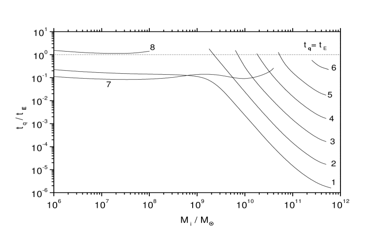
Figure 1: The ratio $t_{q}(M_{i})/t_{E}$ as a function of the initial MBH mass $M_{i}$. Curves labeled 1 to 6 are based on distribution A for $\eta=$$10^{-1}$, $10^{-2}$, $10^{-3}$, $10^{-4}$, $10^{-5}$, and $10^{-6}$, respectively. Curves 7 and 8 are based on distribution B for $\eta=$$10^{-1}$ and $10^{-2}$, respectively.

In Fig. 1 and Fig. 2, we employ two somewhat different distributions in MBH mass from S98 and name them ‘distribution A’ and ‘distribution B’, which correspond to the power-law and log-Gaussian shape of dispersion, respectively. Fig. 1 presents the results of our numerical computation of the ratio $t_{q}(M_{i})/t_{E}$ for different values of $\eta$ and MBH mass distributions A and B. It should be noted that if $\eta<0.1$, the solution exists not for all values of $M_{i}$. The domain where the solution exists is determined from the condition that the r.h.s of Eq. (2) exceeds its l.h.s. if one puts $X=+\infty$. For those $M_{i}$ which lead to an opposite condition, the number of galactic nuclei with MBHs is not enough to explain, in the framework of our model, the distribution function of quasars in $M_{B}$ and $z$, even if these MBHs stay in an active quasar state during the maximum possible time $t_{q}\sim 3t_{E}$. The solution only exists at $\eta>7\cdot 10^{-7}$ for BH mass distribution A and at $\eta>6\cdot 10^{-3}$ for distribution B. A single-valued mapping $M_{i}\to M_{h}$ breaks up on the left end of curves 2 to 6.

Fig. 1 demonstrates the main result of this work: distributions of MBHs and quasars in mass are connected by one-to-one correspondence through the whole range of the observed masses only for $\eta\sim 0.1$, both for the distribution A (curve 1) and B (curve 7). This concordance breaks down for a certain range of MBH masses, viz. the solution of Eq. (2) does not exist if $\eta\ll 0.1$. Nevertheless, the jumps of the $\eta$ value are not excluded on the boundary of the domain, where the solution exists. Similar jumps seem to be quite natural if MBHs in the different mass ranges are formed by different ways (e.g., by collapse of massive gas clouds, stellar clusters, etc., see review by Rees 1984) and so there are various accretion regimes with different values of $\eta$. If such jumps indeed take place, transitions between the curves of each of distributions A and B are possible. These transitions must be smoothed because the MBHs formed by different ways would coexist in some mass range(s). The most probable value of $\eta$ established above is $\eta\sim 0.1$, which corresponds to curves 1 and 7 in Fig. 1. For both these curves, the relationship $t_{q}<t_{E}$ is carried out and therefore the BH mass growth is not substantial – it generally does not exceed a value comparable to the initial BH mass, and for $M_{h}>10^{7}~{}{\rm M}_{\odot}$ it is negligible.

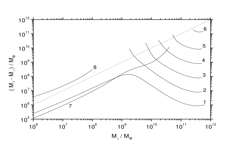
Figure 2: The accreted mass, $M_{f}-M_{i}$, as a function of the initial mass $M_{i}$. The curves are labeled in the same way as in Fig. 1.

References

- (1) Kormendy J., Richstone D., 1995, ARA&A, 33, 581
- (2) Magorrian J. et al., 1997, astro-ph/9708072
- (3) Bahcall J.N., Kirhakos, S., Saxe, D.H., Schneider, D.P. 1997, ApJ 479, 642
- (4) Ozernoy L.M. 1998, Bull. Amer. Astr. Soc. 30, 1286
- (5) Salucci P. et al., 1998, astro-ph/9811102, astro-ph/9812485
- (6) Haehnelt M.G., Natarajan P., Rees M. J., 1997, astro-ph/9712259
- (7) Boyle B.J., 1991, in Proc. Texas/ESO–CERN Symp. on Relativistic Astrophysics, Cosmology, Fundamental Physics, ed. Barrow J.D., Mestel L., Thomas P.A., p. 14