Deprojection of light distributions of nearby systems: perspective effect and non-uniqueness

Abstract

Deriving the 3-dimensional volume density distribution from a 2-dimensional light distribution of a system yields generally non-unique results. The case for nearby systems is studied, taking into account the extra constraints from the perspective effect. It is shown analytically that a new form of non-uniqueness exists. The Phantom Spheroid (PS) for a nearby system preserves the intrinsic mirror symmetry and projected asymmetry of the system while changing the shape and the major-axis orientation of the system. A family of analytical models are given as functions of the distance ($D_{0}$) to the object and the amount ($\gamma$) of the PS density superimposed. The range of the major axis angles is constrained analytically by requiring a positive density everywhere. These models suggest that observations other than surface brightness maps are required to lift the degeneracy in the major axis angle and axis ratio of the central bar of the Milky Way.

1 Introduction

Deprojection of galaxies from the observed light distribution on the sky plane to the intrinsic 3-dimensional volume luminosity distribution is one of the basic problems of astronomy. It is common knowledge that the deprojected results are generally non-unique because of the freedom of distributing stars along any line of sight. The best example is that a round distribution in projection may correspond to any intrinsically prolate object pointing towards us. Likewise we cannot tell from observed elliptical isophotes whether the object is an intrinsically oblate bulge or a triaxial bar if both are edge-on and at infinity (Contopoulos 1956).

The perspective effect of nearby triaxial objects, however, does make them appear different from an oblate object. The best example for this is the famous left-to-right asymmetry of the dereddened light distribution of the Milky Way bulge when plotted in the Galactic $(l,b)$ coordinates, which led Blitz & Spergel (1991) to conclude that the Galactic bulge is in fact an almost edge-on bar, pointing at an angle from the Sun. They divide the Galaxy into a left and a right part with the $l=0^{o}$ plane, which passes the Sun-center line and the rotation axis of the Galaxy. When folded along the $l=0^{o}$ line the surface brightness map $I(l,b)$ is decomposed into two independent maps: an asymmetry map $\left[I(l,b)-I(-l,b)\right]/2$ by subtracting the $l<0^{o}$ side from the $l>0^{o}$ side, and a symmetric map $\left[I(l,b)+I(-l,b)\right]/2$ by adding up the two sides. The signal in the asymmetry map, they explain, is because the right hand side ($l>0^{o}$) of the bar is nearer to us and the perspective effect makes it appear slightly bigger than the left hand side ($l<0^{o}$). A simple sketch of the geometry is shown in the top diagram of Fig. 1.

The perspective effect allows Binney & Gerhard (1996) and Binney, Gerhard & Spergel (1997) to derive a non-parametric volume density distribution of the inner Galaxy. The key element in their method is to impose mirror symmetry for the bulge part of the Galaxy to allow for a triaxial bar, and central symmetry for the disk part so to allow for the spiral arm. Although shifting material along the same line of sight does not alter the isophotes, it spoils the symmetry of the object. Their numerical experiments suggest that the COBE map is consistent with a range of bar models with the bar major axis pointing some $15^{o}-35^{o}$ from the Sun.

Unfortunately there is a lack of analytical studies of general non-uniqueness for nearby objects. This is compared to a series of papers exploiting the analytical properties of konuses in the deprojection of external axisymmetric systems (Rybicki 1986, Palmer 1994, Kochanek & Rybicki 1996, van den Bosch 1997, Romanowsky & Kochanek 1997). A small amount of konuses, as christened by Gerhard & Binney (1996) for a well-studied class of artificial density models with zero surface brightness, can be added to a galaxy at infinity without perturbing its isophotes or creating negative-density zones.

This paper is a first attempt to give an analytical description of the degeneracy in deprojecting the light distribution of a general nearby system. To ensure our arguments are not diluted by the necessary mathematics, we will first introduce the so-called phantom spheroidal (PS) density in §2 and describe its effect on non-uniqueness in words and illustrations. The more mathematical aspects of the problem are given in §3-§5, where we describe the properties of PS densities and how to generate them. We will then briefly discuss the relations to the Milky Way bar in §6, and relations with well-known non-uniqueness of extragalactic objects in §7. We conclude in §8. Some additional results on the major axis angle and a generalization of the phantom density are given in the Appendix.

2 Phantom Spheroid: a compromise between mirror symmetry and perspective effect

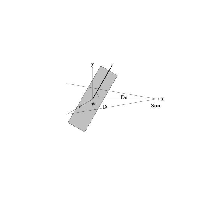
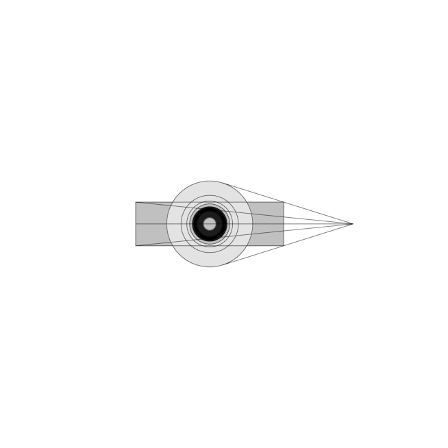
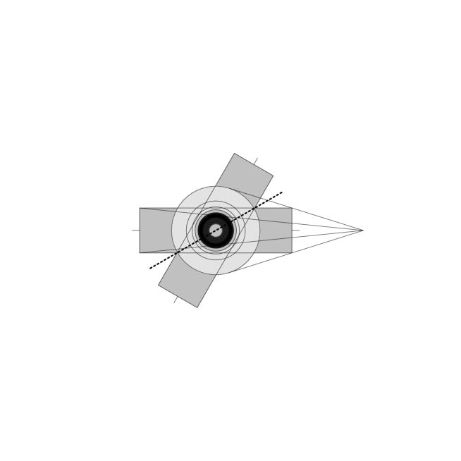
Figure 1: Top panel: the $xy$ cross section of a uniform cigar-shaped bar at distance $D_{0}$ with its major axis tilted at an angle $\alpha$ counterclockwise from the Sun-object center line. The coordinates of a point in the $xy$ plane can also be prescribed by its line of sight distance $D$, the impact parameter $w$, and the distance $r$ to the object center. Middle panel: a phantom spheroid (PS). Bottom panel: a superposition of the above two bodies. Several line-of-sight pathes from the Sun are drawn in thin solid lines. The PS is made by putting a clone of the cigar-shaped bar to an end-on geometry, and subtracting from it a stratified ball-shaped bulge of the same angular size and projected intensity. Adding such a PS to the cigar-shaped bar in the top diagram has no effect on the latter’s projected intensity, but rotates the mirror plane of the spatial distribution to the dotted line in the middle at an angle ${\alpha\over 2}$ from the Sun-center line.

A phantom density is a model with both positive and negative density regions and a zero net surface brightness to an observer at some distance away. An example of a phantom density is illustrated in the middle diagram of Fig. 1, where we tailor the radial profile of a stratified ball-shaped bulge in such a way so to have the same angular size and projected intensity as a uniform cigar-shaped bar placed end-on. Subtracting the ball-shaped bulge from the cigar-shaped bar yields a Phantom Spheroid (PS). The thin dark ring in the bulge is a density peak, corresponding to the line of sight to the far edge of the cigar-shaped bar, a direction where the depth and the projected intensity of the bar are at maximum. The fall-off of density towards the edge of the bulge corresponds to the ever-decreasing depth of the cigar-shaped bar with increasing impact parameter of the line of sight.

The problem with this simple cigar model is that if we superimpose this unphysical component on any physical density distribution, say, an ellipsoidal bar with a Gaussian radial profile, we get a new density with generally twisted density patterns. So while the added cigar component is invisible from the observer’s perspective, it generally spoils the mirror symmetry of the system.

The exception is, as shown in the lower diagram of Fig. 1, when the superimposed end-on cigar is a clone of the original cigar, in which case the final density of the twin should have mirror symmetry with respect to a new plane (the dotted line) which is just in between the Sun-center line and the major axis of the original cigar. In this case the mirror symmetry is preserved, only the symmetry plane is rotated. Subtracting the round bulge has no further effect on the symmetry plane, but will take away any trace of transformation in the map of the integrated light. Thus a PS which rotates the symmetry axes and is invisible in projection can be obtained by placing the original prolate cigar end-on and then subtracting off a round bulge.

We can apply the same trick to oblate systems, such as disks, because a face-on disk mimics a spherical distribution the same way a prolate cigar bar does. So suppose the original model is a disk tilted at an angle $\alpha$ from the line of sight. Adding a face-on clone of the disk will put the mirror plane of the twin disks at an angle ${\alpha\over 2}$. By subtracting off a spherical model we can take away any effect of the face-on clone in the projected brightness map. In fact this kind of non-uniqueness applies any spheroidal (i.e. prolate or oblate) distribution with any radial profile since our arguments about non-uniqueness is independent of the aspect ratio and density profile of the bar. For example, the original model may consists of a small spheroidal perturbation on top of a large positive spherical component, both with general smooth radial profiles.

Despite these generalizations, the models are restricted in the sense that the models come only as twins with identical projected brightness distribution. This is compared to non-uniqueness in the extragalactic systems, such as konuses, where we find a family of models with indistinguishable surface brightness maps with a tunable amount of konuses. The models here are also likely to have large zones of negative density because we subtract off a significant amount of matter with a spherical distribution. This problem can be softened if our original model has a large positive smooth spherical component to start with.

3 Method for generating general Phantom Spheroids

Let’s first set up a rectangular coordinate system $(x,y,z)$ centered on the object with the $x$ axis pointing towards the observer. In this coordinate system the observer is at $(D_{0},0,0)$, where $D_{0}$ is the observer’s distance to the object center. From the observer’s perspective the surface brightness map of the system is most conveniently specified by two angles $(l^{\prime},b^{\prime})$, which are the equivalent of the Galactic coordinate system with the $b^{\prime}=z=0$ plane being the $xy$ plane and the $l^{\prime}=y=0$ plane passing through $z$-axis of the system. In these coordinates the system center and anti-center are in the directions $(l^{\prime},b^{\prime})=(0,0)$ and $(\pi,0)$. A point $(x,y,z)$ in rectangular coordinates can thus be specified by the distance $D$ to the observer along the line of sight $(l^{\prime},b^{\prime})$ with

$$x=D_{0}-D\cos b^{\prime}\cos l^{\prime},~{}~{}~{}y=D\cos b^{\prime}\sin l^{\prime},~{}~{}~{}z=D\sin b^{\prime}.$$ (1)

The impact parameter $w$ with respect to the object center is given by

$$w=D_{0}\sqrt{\left(\sin b^{\prime}\right)^{2}+\left(\cos b^{\prime}\sin l^{\prime}\right)^{2}}$$ (2)

for the line of sight $(l^{\prime},b^{\prime})$. The distance $r$ to the center of the object at $(0,0,0)$ is given by

$$r=\sqrt{x^{2}+y^{2}+z^{2}}=\sqrt{\Delta^{2}+w^{2}},~{}~{}~{}\Delta=D-\sqrt{D_{0}^{2}-w^{2}},$$ (3)

where $\Delta$ is the offset distance from the tangent point. The rectangular coordinates can also be expressed in terms of $w$ and $D$ with

$$x=D_{0}-D\sqrt{1-{w^{2}\over D_{0}^{2}}},~{}~{}~{}\sqrt{y^{2}+z^{2}}={D\over D_{0}}w.$$ (4)

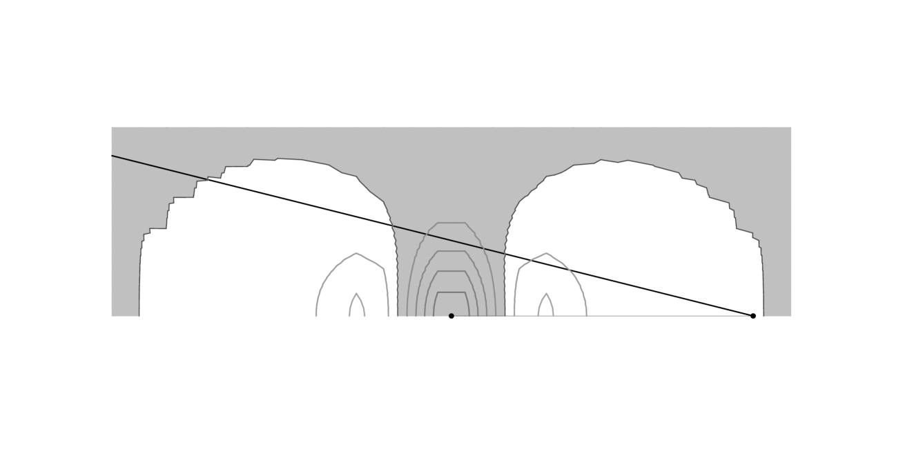
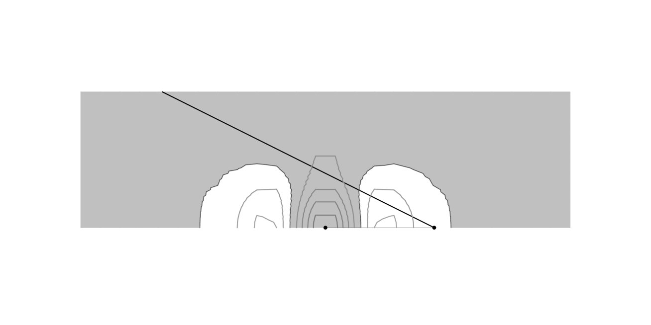
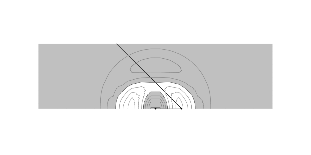
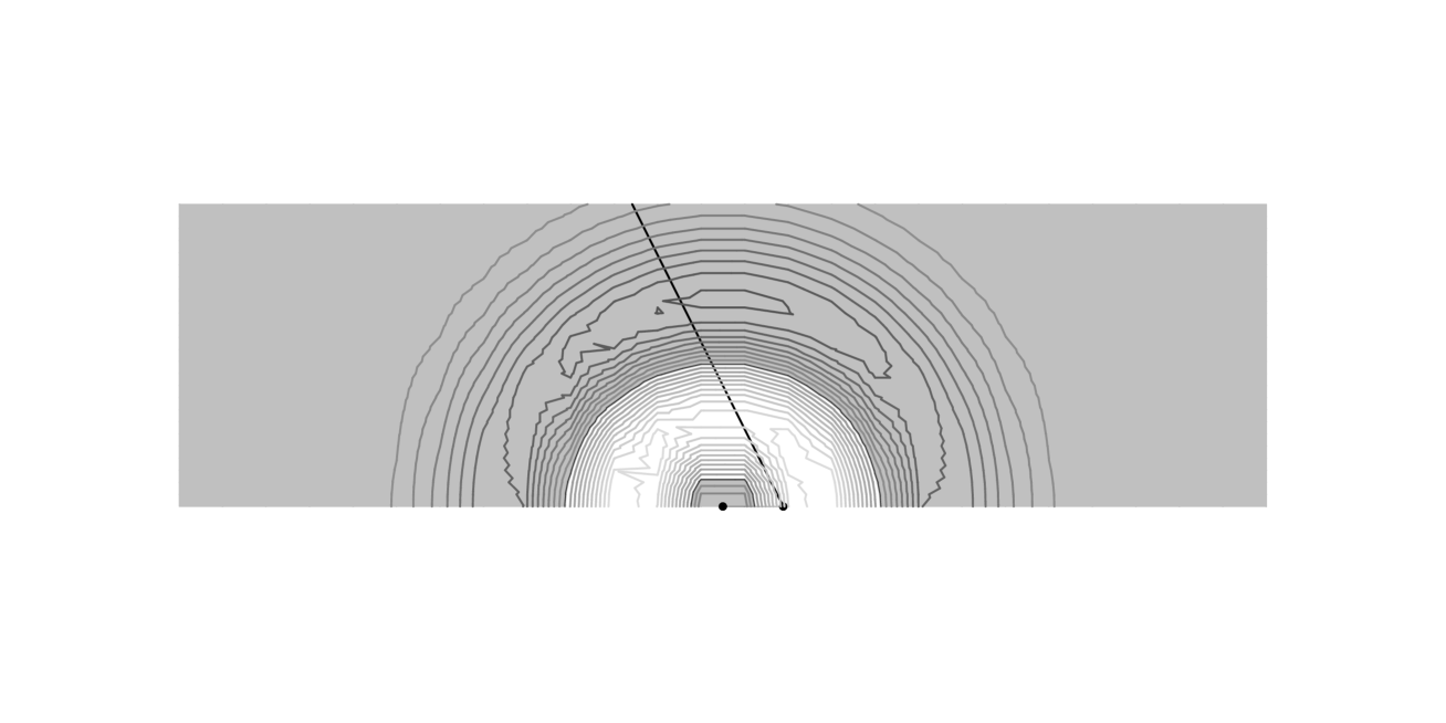
Figure 2: Cross sections of several phantom spheroidal density models (cf. eq. 45) in terms of $x$ (horizontal axis) vs. $\sqrt{y^{2}+z^{2}}$ (vertical axis). The distributions are rotationally symmetric around the Sun-center axis (i.e., the horizontal $x$-axis). The shaded regions are negative density zones of the PS. We show several locations of the observer (solid circle to the right) at $D_{0}=4a,2a,a,0.5a$ (from top to bottom) from the object center (solid circle to the lower left corner) and draw a line of sight which intersects the $x=0$ plane at a radius $a$. The amount of light adds up to zero along any line from the observer’s perspective.

Most generally our phantom spheroid $F(x,y,z)$ is made by subtracting from an end-on prolate distribution $P(|x|,\sqrt{y^{2}+z^{2}})$ a spherical bulge $S(r)$ with matching surface brightness, i.e.,

$$\int_{0}^{\infty}\!\!F(x,y,z)dD=0,~{}~{}~{}F(x,y,z)\equiv P(|x|,\sqrt{r^{2}-x^{2}}=\sqrt{y^{2}+z^{2}})-S(r),$$ (5)

where $\int_{0}^{\infty}\!\!dD$ is an integration along any line-of-sight direction, say, $(l^{\prime},b^{\prime})$. Clearly $F(x,y,z)$ is an even function of $x$, $y$ and $z$ with

$$F(x,y,z)=F(x,-y,z)=F(x,y,-z)=F(x,-y,-z)=F(-x,y,z),$$ (6)

and in fact has rotational symmetry around the $x$-axis. The total luminosity of a phantom $L_{PS}$ is given by

$$L_{PS}\equiv\int\!\!d^{3}{\bf r}F(x,y,z)=L_{P}-L_{S},~{}~{}~{}L_{P}\equiv\int\!\!d^{3}{\bf r}P(|x|,\sqrt{y^{2}+z^{2}}),~{}~{}~{}L_{S}\equiv\int\!\!d^{3}{\bf r}S(r).$$ (7)

As we will show later a phantom spheroid can have a net luminosity because the total luminosity of the prolate component $L_{P}$ is only approximately that of the spherical component $L_{S}$ with the difference being infinitely small when the observer is infinitely far away from the object.

Let $J(w)$ be the light intensity of the prolate distribution $P(|x|,\sqrt{y^{2}+z^{2}})$ integrated over a line of sight with impact parameter $w$, including both the forward direction and the backward direction, then

$$J(w)\equiv\int_{-\infty}^{\infty}\!\!P(|x|,\sqrt{y^{2}+z^{2}})dD,$$ (8)

where $x,y,z$ can be expressed in terms of $w$ and $D$ using eq. (3) and eq. (4). Once $J(w)$ is computed from the integration of $P(|x|,\sqrt{y^{2}+z^{2}})$, our task is to find a spherical bulge $S(r)$ such that

$$J(w)=\int_{-\infty}^{\infty}\!\!S(r)dD.$$ (9)

This can be done using the Abel transformation

$$S(r)=-{1\over\pi}\int_{r}^{\infty}\!\!{dJ(w)\over dw}{dw\over\sqrt{w^{2}-r^{2}}}.$$ (10)

The inversion uses effectively a variation of the well-known Eddington formula for deprojecting a spherical system (cf. Binney & Tremaine 1987). Thus we find a general expression for the phantom spheroid (PS); there is no restriction on the radial profile or the axis ratio of the prolate distribution $P(|x|,\sqrt{y^{2}+z^{2}})$, and in fact it is allowed to be oblate. Any PS can also lead to a family of PS densities because new PS can be generated by applying a linear operator to an old PS. For example, suppose $F(x,y,z)$ has a free parameter $\beta$, then ${\partial\over\partial\beta}F(x,y,z)$ is also a PS (cf. Appendix B).

To reformulate the results in the previous section about the “twin bars” in mathematical terms, we define a new set of rectangular coordinates $(x_{\alpha},y_{\alpha},z_{\alpha})$ which relate to the rectangular coordinates $(x,y,z)$ by a rotation around the $z$-axis (i.e., in the $xy$ plane) by an angle $\alpha$ with

$$(x_{\alpha},y_{\alpha},z_{\alpha})=(x\cos\alpha+y\sin\alpha,-x\sin\alpha+y\cos\alpha,z).$$ (11)

The rotation transformation has the property that

$$x_{\alpha}^{2} = x_{\alpha/2}^{2}\cos^{2}{\alpha\over 2}+y_{\alpha/2}^{2}\sin^{2}{\alpha\over 2}+2x_{\alpha/2}y_{\alpha/2}\sin{\alpha\over 2}\cos{\alpha\over 2},$$ (12)

$$x^{2} = x_{\alpha/2}^{2}\cos^{2}{\alpha\over 2}+y_{\alpha/2}^{2}\sin^{2}{\alpha\over 2}-2x_{\alpha/2}y_{\alpha/2}\sin{\alpha\over 2}\cos{\alpha\over 2}.$$

In these notations we let $P(|x_{\alpha}|,\sqrt{r^{2}-x_{\alpha}^{2}})$ denote any general prolate bar, made by rotating its end-on twin bar $P(|x|,\sqrt{r^{2}-x^{2}})$ to an angle $\alpha$ from the line of sight in the $xy$ plane. Then we can always design a triaxial object

$$T(|x_{\alpha/2}|,|y_{\alpha/2}|,|z_{\alpha/2}|)\equiv P(|x_{\alpha}|,\sqrt{r^{2}-x_{\alpha}^{2}})+P(|x|,\sqrt{r^{2}-x^{2}})-S(r),$$ (13)

where $S(r)$ is given by eqs. (8) and (10) so that the triaxial object $T(|x_{\alpha/2}|,|y_{\alpha/2}|,|z_{\alpha/2}|)$ has exactly the same surface brightness as the prolate bar $P(|x_{\alpha}|,\sqrt{y_{\alpha}^{2}+z_{\alpha}^{2}})$, i.e.,

$$\int_{-\infty}^{\infty}\!\!P(|x_{\alpha}|,\sqrt{y_{\alpha}^{2}+z_{\alpha}^{2}})dD=\int_{-\infty}^{\infty}\!\!T(|x_{\alpha/2}|,|y_{\alpha/2}|,|z_{\alpha/2}|)dD.$$ (14)

To verify the mirror symmetries of the distribution $T(|x_{\alpha/2}|,|y_{\alpha/2}|,|z_{\alpha/2}|)$, simply substitute eq. (12) to eq. (13) and apply the transformation $x_{\alpha/2}\rightarrow-x_{\alpha/2}$ or $y_{\alpha/2}\rightarrow-y_{\alpha/2}$. In both cases we have $|x_{\alpha}|\rightarrow|x|$. The mirror symmetry with $z_{\alpha/2}=0$ plane is obvious because $T(|x_{\alpha/2}|,|y_{\alpha/2}|,|z_{\alpha/2}|)$ is an even function of $z_{\alpha/2}$, which comes in only through the $r^{2}=x_{\alpha/2}^{2}+y_{\alpha/2}^{2}+z_{\alpha/2}^{2}$ factor. Note that we do not lose generality by choosing the rotation to be around the $z$-axis since there is no prefered direction in the $yz$ plane of the prolate bar $P(|x|,\sqrt{y^{2}+z^{2}})$.

To summarize the main result here, we have shown that any prolate bar has a triaxial counterpart with identical surface brightness but half the viewing angle. An immediate question is to what extent we can build triaxial models with the viewing angle varying continuously.

4 A general sequence of triaxial models with identical surface brightness

In the following we will construct a subclass of these phantom spheroids which preserve the mirror symmetry for a continuous sequence of fairly general triaxial models. We do not know whether such constructions exist for all triaxial models, but it does exist if the triaxial density distribution $\nu_{0}(x,y,z)$ can be decomposed to a spherical part $G(r)$ and a non-spherical part $p(r)Q_{0}(x,y,z)$, i.e.,

$$\nu_{0}(x,y,z)=G(r)+p(r)Q_{0}(x,y,z),$$ (15)

where the only restriction is that $Q_{0}(x,y,z)$ is a quadratic function of rectangular coordinates, i.e.,

$$Q_{0}\equiv c_{11}x^{2}+c_{22}y^{2}+c_{33}z^{2}+2c_{12}xy+2c_{23}yz+2c_{31}zx.$$ (16)

There is complete freedom with the functional forms of $G(r)$ and $r^{2}p(r)$, which are the the radial profiles of the spherical component and the non-spherical component respectively. These models are also triaxial by construction because surfaces of constant $Q_{0}$ are ellipsoidal isosurfaces. The symmetry planes of the ellipsoid can be oriented to any direction by changing the elements of the symmetric matrix $c_{ij}$ where $c_{ij}=c_{ji}$ and the indices $i$ and $j$ are from 1 to 3. The total luminosity of the model, $L_{0}$, is given by

$$L_{0}\equiv\int\!\!d^{3}{\bf r}\nu_{0}(x,y,z)=4\pi\int_{0}^{\infty}\!\!drr^{2}G(r)+{4\pi\over 3}\sum_{i=1}^{3}c_{ii}\int_{0}^{\infty}\!\!drr^{4}p(r).$$ (17)

We define $I(l^{\prime},b^{\prime})$ as the surface brightness integrated along both the $(l^{\prime},b^{\prime})$ direction and the opposite $(\pi+l^{\prime},-b^{\prime})$ direction. The central surface brightness, $I_{0}$, integrated along the $x$-axis (i.e. with $x$ from $-\infty$ to $\infty$ and $y=z=0$) is given by

$$I_{0}\equiv\int_{-\infty}^{\!\infty}\!\!\nu_{0}(x,0,0)dx=\int_{-\infty}^{\!\infty}\!\!\left[G(r)+c_{11}r^{2}p(r)\right]dr,~{}~{}~{}r=x,$$ (18)

where $r$ and $x$ are interchangeable dummy variables for the integrations.

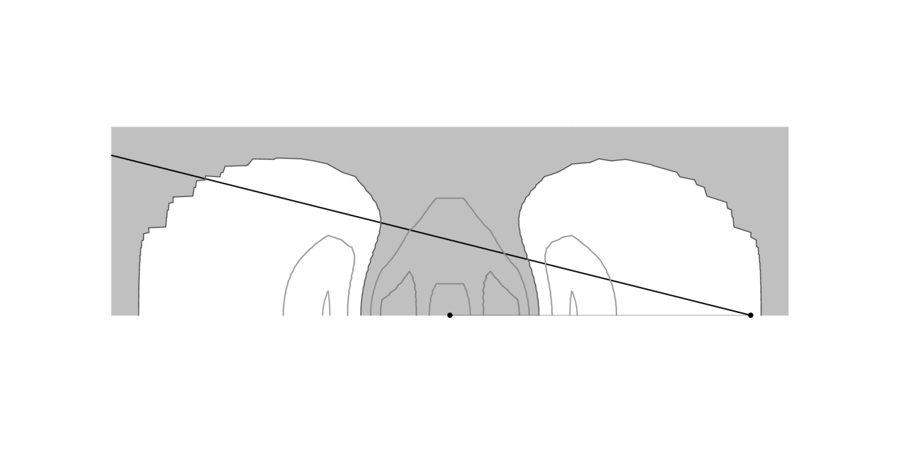
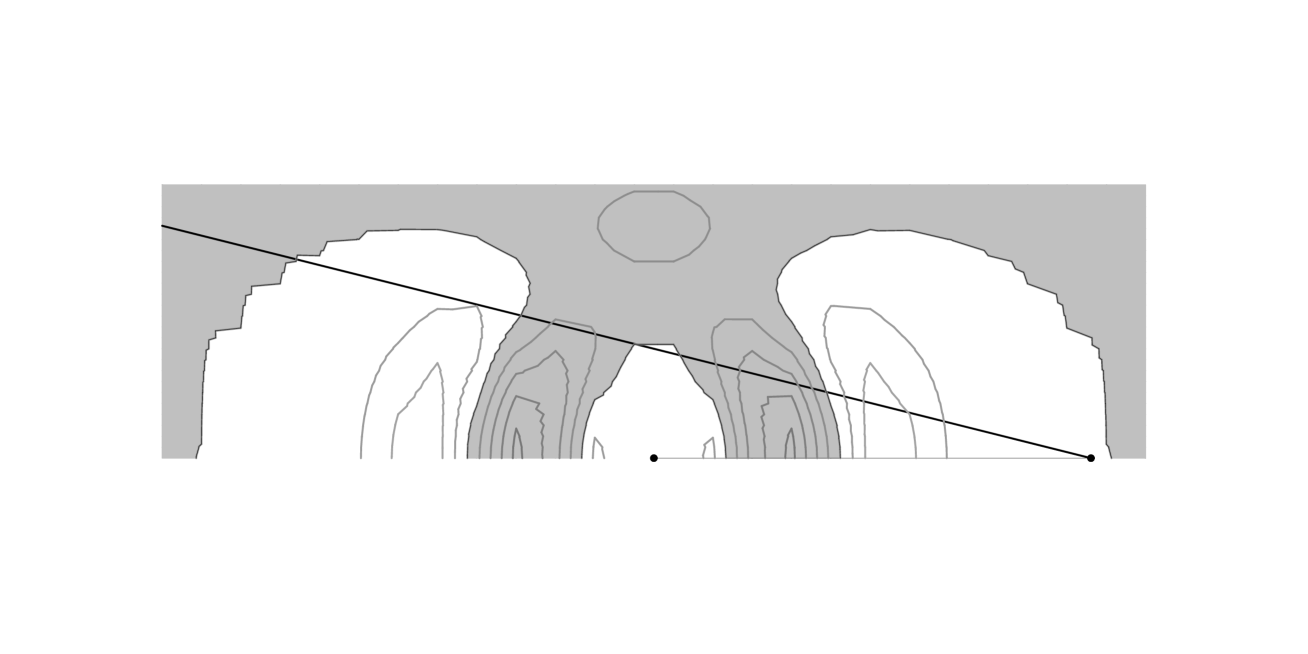
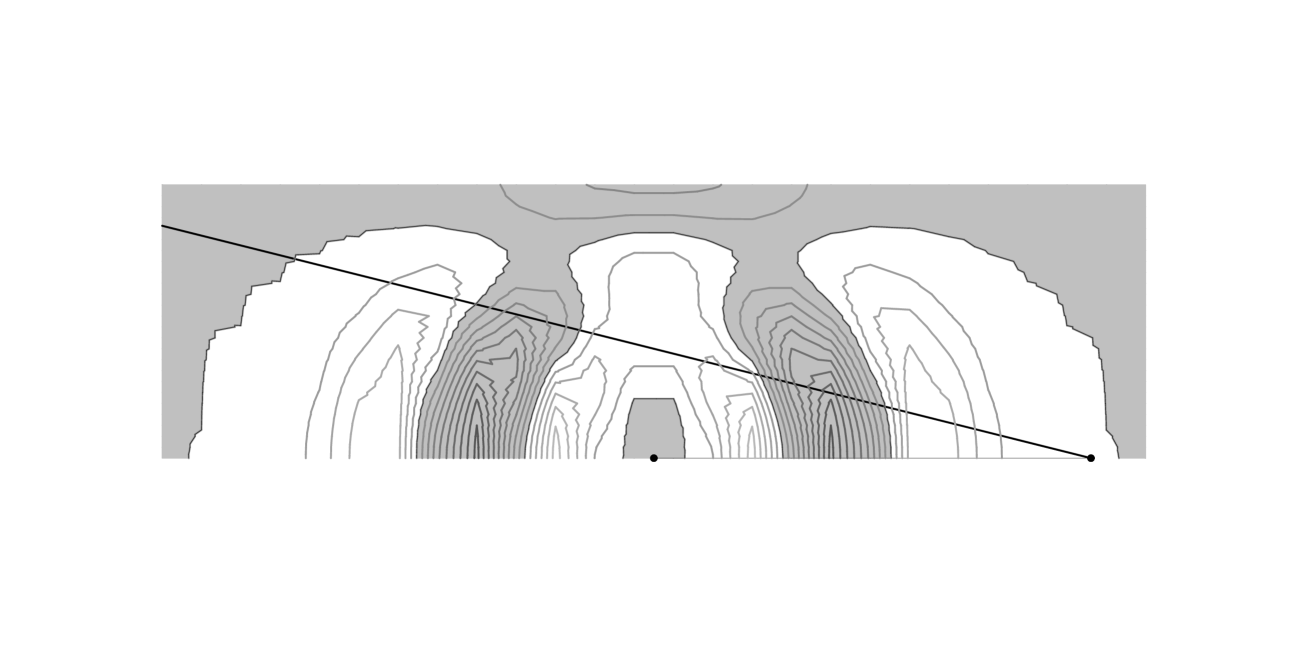
Figure 3: Same as the previous figure but for the new phantom spheroidal densities $F_{1}$, $F_{2}$ and $F_{3}$. (cf. eq. 46) with the observer at $D_{0}=4a$.

For the above triaxial model we can construct a phantom spheroid $F(x,y,z)$ with

$$F(x,y,z)=P(|x|,\sqrt{y^{2}+z^{2}})-S(r),~{}~{}~{}P(|x|,\sqrt{y^{2}+z^{2}})=x^{2}p(r),$$ (19)

where the spherical component $S(r)$ is computed from (cf. eq. 10)

$$S(r)=-{1\over\pi}\int_{r}^{\infty}\!\!{dJ(w)\over dw}{dw\over\sqrt{w^{2}-r^{2}}},~{}~{}~{}J(w)=\int_{-\infty}^{\infty}\!\!x^{2}p(r)dD,$$ (20)

so to cancel the $P(|x|,\sqrt{y^{2}+z^{2}})$ component in the projected light distribution. Clearly $F(x,y,z)$ is a spheroidal distribution with axial symmetry around the Sun-center axis since it is made by subtracting from a prolate distribution $x^{2}p(r)$ a spherical distribution $S(r)$ of identical surface brightness. Let $J_{0}$ be the line of sight integration of either the spherical $S(r)$ or the prolate $x^{2}p(r)$ distribution along the $x$-axis, then

$$J_{0}\equiv J(0)=\int_{-\infty}^{\!\infty}\!\!S(r)dr=\int_{-\infty}^{\!\infty}\!\!r^{2}p(r)dr.$$ (21)

The total luminosity of the phantom spheroid, $L_{PS}$, is given by

$$L_{PS}=L_{P}-L_{S},~{}~{}~{}L_{P}={4\pi\over 3}\int_{0}^{\infty}\!\!drr^{4}p(r),~{}~{}~{}L_{S}=4\pi\int_{0}^{\infty}\!\!drr^{2}S(r).$$ (22)

Adding a fraction $\gamma$ of the above phantom spheroid to our original model $\nu_{0}(x,y,z)$ we get a new model

$$\nu_{\gamma}(x,y,z)=\nu_{0}(x,y,z)+F(x,y,z)\gamma,$$ (23)

which should have identical surface brightness map as the old one. Rearranging the terms we find

$$\nu_{\gamma}(x,y,z)=G_{\gamma}(r)+p(r)Q_{\gamma}(x,y,z),$$ (24)

where

$$G_{\gamma}\equiv G(r)-\gamma S(r),~{}~{}~{}r=\sqrt{x^{2}+y^{2}+z^{2}},$$ (25)

and

$$Q_{\gamma}(x,y,z)\equiv Q_{0}(x,y,z)+\gamma x^{2}=(\gamma+c_{11})x^{2}+c_{22}y^{2}+c_{33}z^{2}+2c_{12}xy+2c_{23}yz+2c_{31}zx.$$ (26)

So the new model is very similar to the old model. Both are superpositions of a spherical component and a triaxial perturbation; the triaxiality is guaranteed by the fact that $Q_{\gamma}(x,y,z)$ prescribes ellipsoidal isosurfaces. In general the orientation of the object is a function of $\gamma$ given by

$$\cot 2\alpha_{xy}={\gamma+c_{11}-c_{22}\over 2c_{12}},~{}~{}~{}\cot 2\alpha_{xz}={\gamma+c_{11}-c_{33}\over 2c_{13}},~{}~{}~{}\cot 2\alpha_{yz}={c_{22}-c_{33}\over 2c_{23}},$$ (27)

where $\alpha_{xy}$ and $\alpha_{xz}$ are the tilt angles of the object from the the line of sight in the $xy$ plane (i.e., the $z=0$ cut) and the $xz$ plane (i.e. the $y=0$ cut), and $\alpha_{yz}$ is the tilt angle counting from the $y$-axis in the $yz$ plane (i.e., the $x=0$ cut). We make two comments here. First the orientation in the $yz$ plane is not affected by the phantom spheroid because the latter is generally rotationally symmetric around in the $yz$ plane (cf. eq. 19). Second the directions of the principal axes of the triaxial object should generally be eigenvectors of the $3\times 3$ matrix $c_{ij}+\gamma\delta_{11}$ with $i,j=1,2,3$. The corresponding eigenvalues are generally the three roots of a cubic equation. In practice, it is more convenient to speak of the orientation of the object in terms of the angles $\alpha_{xy}$ and $\alpha_{xz}$, which prescribe the major axes in the $xy$ and $xz$ plane cuts.

There are, however, limits to $\gamma$, the amount of PS that we can add to a model. A physical density model must have a positive phase space density and must be stable. This, in principle, set limits on the non-uniqueness if we can build dynamical (numerical) models for a sequence of potentials with different $\gamma$. In practice stringent limits can already be obtained from the minimal requirement that the volume density of a physical model is everywhere positive, i.e.,

$$\nu_{\gamma}(x,y,z)=\left[G(r)+p(r)Q_{0}(x,y,z)\right]+\gamma\left[x^{2}p(r)-S(r)\right]\geq 0.$$ (28)

This generally involves (numerically) searching over a 3-dimensional space $(x,y,z)$ for the minimum of the density $\nu_{\gamma}(x,y,z)$, and finding the range of $\gamma$ which brings the minimum above zero; for edge-on models, this can be reduced to a search in 2-dimensional space (see Appendix A).

Nevertheless there are many easy-to-use variations of the positivity equation. For example, a positive volume density at the object center requires (cf. eq. 28)

$$\nu_{\gamma}(0,0,0)=G_{\gamma}(0)=G(0)-\gamma S(0)\geq 0,$$ (29)

while a less interesting condition can come from requiring a positive total luminosity of the object $L_{\gamma}$, given by

$$L_{\gamma}\equiv\int\!\!d^{3}{\bf r}\nu_{\gamma}(x,y,z)=L_{0}+\gamma L_{PS}\geq 0.$$ (30)

A stringent set of conditions can be derived by computing the following moments of the density distribution. This is done by first multiplying both sides of eq. (28) by a factor $r^{k}$, where $k$ can be 0, 1, 2 etc.. Then integrate over $r$ along a general direction ${\bf n}=(n_{1},n_{2},n_{3})$ through the origin, i.e., from $r=-\infty$ to $r=\infty$ with $(x,y,z)=(n_{1}r,n_{2}r,n_{3}r)$. We find

$$\int_{-\infty}^{\!\infty}\!\!\nu_{\gamma}(n_{1}r,n_{2}r,n_{3}r)r^{k}dr=\int_{-\infty}^{\!\infty}\!\!\left[G(r)+c_{nn}r^{2}p(r)\right]r^{k}dr+\int_{-\infty}^{\!\infty}\!\!\left[\gamma n_{1}^{2}r^{2}p(r)-\gamma S(r)\right]r^{k}dr,$$ (31)

where

$$n_{1}^{2}+n_{2}^{2}+n_{3}^{2}=1,~{}~{}~{}c_{nn}\equiv\sum_{i,j=1}^{3}c_{ij}n_{i}n_{j}.$$ (32)

Requiring the $k=0$ moment of the density $\nu_{\gamma}(x,y,z)$ to be positive we have

$$\int_{-\infty}^{\!\infty}\!\!\nu_{\gamma}(n_{1}r,n_{2}r,n_{3}r)dr=I_{0}+\left[\left(\sum_{i,j=1}^{3}c_{ij}n_{i}n_{j}-c_{11}\right)-\left(n_{2}^{2}+n_{3}^{2}\right)\gamma\right]J_{0}\geq 0,$$ (33)

where we have substituted in the definitions for $I_{0}$ and $J_{0}$ (cf. eqns. 18 and 21). Eq. (33) generally yields a necessary upper limit on $\gamma$, and the limit is most stringent when the line $(x,y,z)=(n_{1}r,n_{2}r,n_{3}r)$ is the minor axis of the model. For example, along the $y$-axis with $(n_{1},n_{2},n_{3})=(0,1,0)$ we have

$$2c_{12}\cot 2\alpha_{xy}=\gamma+c_{11}-c_{22}\leq{I_{0}\over J_{0}}$$ (34)

where we express the constraint in terms of the tilt angle $\alpha_{xy}$ (cf. eq. 27) as well as $\gamma$. Note we assume $J_{0}>0$, which is generally valid. Likewise along the $z$-axis with $(n_{1},n_{2},n_{3})=(0,0,1)$ we obtain

$$2c_{13}\cot 2\alpha_{xz}=\gamma+c_{11}-c_{33}\leq{I_{0}\over J_{0}}.$$ (35)

Likewise a positive $k=2$ moment of the density requires

$$4\pi\int_{-\infty}^{\!\infty}\!\!\nu_{\gamma}(n_{1}r,n_{2}r,n_{3}r)r^{2}dr=L_{0}+\left(3\sum_{i,j=1}^{3}c_{ij}n_{i}n_{j}-\sum_{i=1}^{3}c_{ii}\right)L_{P}+\gamma(3n_{1}^{2}L_{P}-L_{S})\geq 0,$$ (36)

where we have substituted in the definitions for $L_{0}$, $L_{P}$ and $L_{S}$ (cf. eq. 17 and 22). Eq. (36) generally yields a necessary lower limit on $\gamma$. For example, along the $x$-axis with ${\bf n}=(1,0,0)$ we have

$$2c_{12}\cot 2\alpha_{xy}+2c_{13}\cot 2\alpha_{xz}=2\gamma+2c_{11}-c_{22}-c_{33}\geq-{L_{\gamma}\over L_{P}},$$ (37)

where we assume the prolate component has a positive luminosity, i.e., $L_{P}>0$, which is generally the case. The r.h.s of eq. (37) can be further simplied in the limit $D_{0}\rightarrow\infty$, i.e., the observer is far away from the object. In this case $L_{\gamma}\rightarrow L_{0}$.

Figure 4: The run of the phantom densities $F$ (top), $F_{1}$ (middle) and $F_{2}$ (bottom) as a function of the radius, where the length is in units of the characteristic length $a$, and the density has units of $\nu_{c}$. The run along the $z$-axis is shown in the left half (the negative half of the horizontal axis), and the run along the $x$-axis is shown in the right half (positive half). Various line styles are for $D_{0}=4a$, $2a$ and $a$ with heavier lines for larger $D_{0}$.

5 A sequence of nearly edge-on triaxial models with a Gaussian profile

The above general results apply to models with any radial profile. To illustrate the model properties effectively, we will use the following smooth triaxial models with a Gaussian radial profile with

$$\nu_{0}(x,y,z)=G(r)+p(r)Q_{0}(x,y,z),~{}~{}~{}G(r)=\nu_{c}e^{-{r^{2}\over 2a^{2}}},~{}~{}~{}p(r)={\nu_{c}\over a^{2}}e^{-{r^{2}\over a^{2}}},$$ (38)

where $a$ is the characteristic scale of the model, $\nu_{c}$ is a characteristic density. These two intrinsic parameters are related to the observable $I_{0}$ (cf. eq. 18) by

$$I_{0}=\int_{-\infty}^{\!\infty}\!\!\nu_{0}(x,0,0)dx=\sqrt{\pi}\left(\sqrt{2}+{c_{11}\over 2}\right)\nu_{c}a,$$ (39)

where $I_{0}$ is effectively the integrated light intensity from both the object center $(l^{\prime},b^{\prime})=(0,0)$ and the anti-center $(l^{\prime},b^{\prime})=(\pi,0)$. While we prefer to keep our derivations as general as possible, wherever quantitative numerical calculations are shown we set the scaling parameters $a$ and $\nu_{c}$ to unity, and use the following set of model parameters

$$c_{11}=c_{22}=-{5\over 6},~{}c_{33}=-{7\over 6},~{}c_{12}={1\over 3},$$ (40)

and

$$c_{31}=c_{23}={1\over 9},$$ (41)

and put the object at the distance

$$D_{0}=4a$$ (42)

unless otherwise mentioned. These parameters describe nearly edge-on models with a characteristic angular size of ${a\over D_{0}}={1\over 4}\sim 15^{o}$; edge-on models have $c_{31}=c_{23}=0$. We will vary $\gamma$ to show the properties of a sequence of models. The results can be generalized qualitatively to all models described by eq. (24).

To find the expression for the phantom spheroid, we substitute eq. (38) in eq. (8). This yields

$$J(w)=\int_{-\infty}^{\infty}\!\!x^{2}p(r)dD=J_{0}e^{-{w^{2}\over a^{2}}}\left(1+{2w^{2}\over a^{2}}-{w^{2}\over D_{0}^{2}}\right),~{}~{}~{}J_{0}={\sqrt{\pi}\over 2}\nu_{c}a,$$ (43)

where $J(w)$ is the integrated intensity of the prolate distribution $x^{2}p(r)$ along the line of sight with the impact parameter $w$, which becomes $J_{0}$ when $w=0$. Applying eq. (10) we find that $S(r)$ reduces to a simple analytical expression,

$$S(r)=-{1\over\pi}\int_{r}^{\infty}\!\!{dJ(w)\over dw}{dw\over\sqrt{w^{2}-r^{2}}}=a^{2}p(r)\left({1\over 2}+{r^{4}\over a^{2}D_{0}^{2}}-{3r^{2}\over 2D_{0}^{2}}\right),$$ (44)

and the PS is given by

$$F(x,y,z)=x^{2}p-S=\nu_{c}e^{-{r^{2}\over a^{2}}}\left[\left({x^{2}\over a^{2}}-{1\over 2}\right)+{a^{2}\over D_{0}^{2}}\left({3r^{2}\over 2a^{2}}-{r^{4}\over a^{4}}\right)\right].$$ (45)

A few examples of the PS are shown in Fig. 2. They vary as a function of characteristic angular size of the object ${a\over D_{0}}$. When the observer is well inside the object, ${a\over D_{0}}\gg 1$, the PS density becomes nearly spherical because of the strong dependence on $r$ (cf. eq. 45). The amplitude changes from $\sim-{a^{2}\over 5D_{0}^{2}}\nu_{c}$ to $\sim{a^{2}\over 5D_{0}^{2}}\nu_{c}$ when $r$ moves from $r=a$ to $r=1.5a$.

We can also generate a sequence of analytical phantom spheroids by repeatedly applying the derivative operator ${1\over 2}{\partial\over\partial\ln a}$ to the original phantom spheroid $F(x,y,z)$ (cf. eq. 45), i.e,

$$F_{n}(x,y,z)=x^{2}p_{n}(r)-S_{n}(r),~{}~{}~{}p_{n}(r)\equiv{\partial^{n}p(r)\over 2^{n}\partial(\ln a)^{n}},~{}~{}~{}S_{n}(r)\equiv{\partial^{n}S(r)\over 2^{n}\partial(\ln a)^{n}}$$ (46)

for $n=1,2,3,...$, where $x^{2}p_{n}(r)$ and $S_{n}(r)$ form a new pair of a prolate bar and a spherical bulge with matching surface brightness. These new analytical PS densities are given in the Appendix B. The contours for these new PS densities are shown in Fig. 3, and radial profiles in Fig. 4. As $D_{0}$ decreases, the amplitude of the radial oscillation of the PS increases, but at the origin we have,

$$F(0,0,0)=-0.5\nu_{c},~{}F_{1}(0,0,0)=F_{2}(0,0,0)=0,$$ (47)

independent of $D_{0}$.

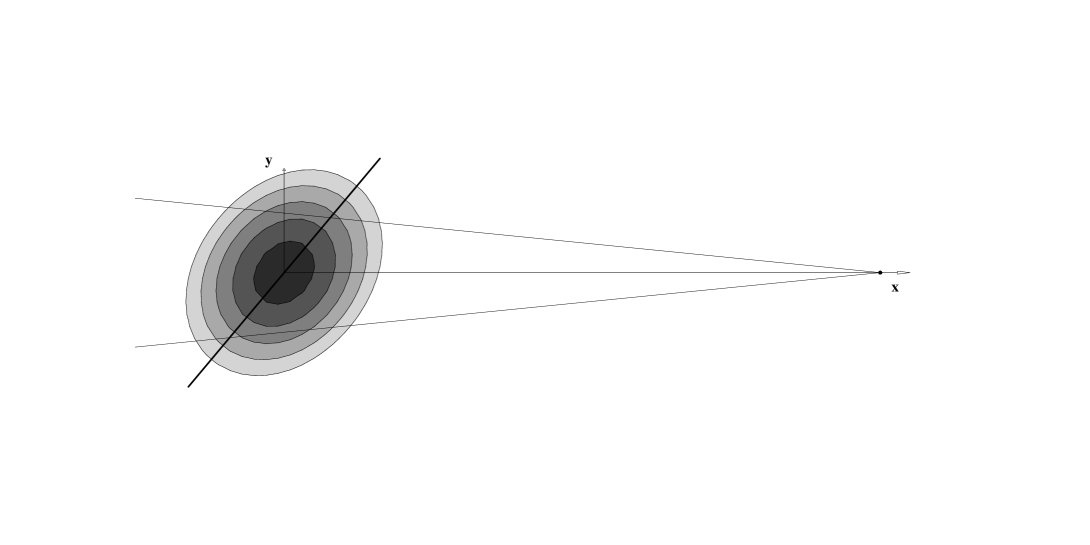
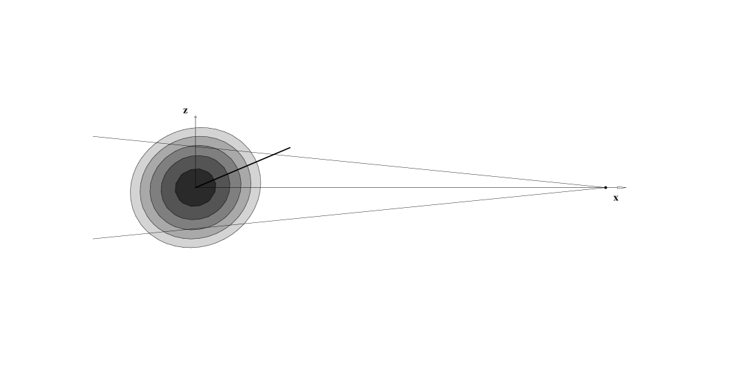
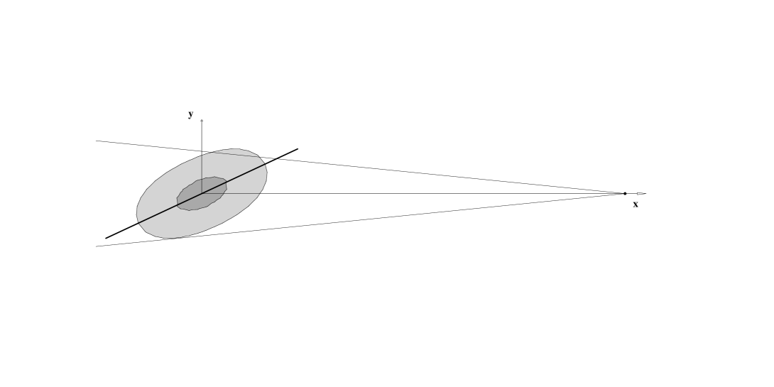
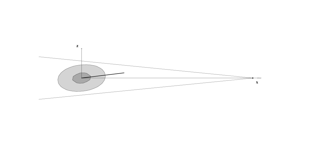
Figure 5: Cross sections of a triaxial nearly edge-on model (cf. eq. 40) with the major axis at $\alpha_{xy}=50^{o}$ from the Sun-center line in the $xy$ plane (top) and at $\alpha_{xz}=23^{o}$ in the $xz$ plane (bottom).

Figure 6: Similar to the previous diagram, but with the major axis at $\alpha_{xy}=25^{o}$ from the Sun-center line in the $xy$ plane (top) and at $\alpha_{xz}=7^{o}$ in the $xz$ plane (bottom). This model appears identical to the previous model in terms of the surface brightness distribution.

Adding the phantom spheroidal density $F(x,y,z)$ to our $\gamma=0$ model (cf. eq. 38), we obtain the general expression for the model density

$$\nu_{\gamma}(x,y,z) = \nu_{c}e^{-{r^{2}\over 2a^{2}}}\left\{1+e^{-{r^{2}\over 2a^{2}}}\left[{Q_{\gamma}\over a^{2}}-{\gamma\over 2}-{\gamma r^{4}\over a^{2}D_{0}^{2}}+{3\gamma r^{2}\over 2D_{0}^{2}}\right]\right\},$$ (48)

$$Q_{\gamma} = (\gamma+c_{11})x^{2}+c_{22}y^{2}+c_{33}z^{2}+2c_{12}xy+2c_{23}yz+2c_{31}zx.$$

The object-observer distance $D_{0}$ can take on any positive value, and the parameters $\gamma$ and $c_{ij}$ can describe the most general orientation of the three symmetry planes of the model (cf. eq. 26). These models have also the nice property that the PS density falls off steeper than the spherical term $G(r)$, meaning that the models are always nearly spherical with a positive, Gaussian profile at large radii.

Figure 7: The run of the volume density along the $x$ (thickest line), $y$ and $z$ (thinnest line) axes for the $\alpha_{xy}=50^{o}$ model (upper curves) and the $\alpha_{xy}=25^{o}$ model (lower curves). The curves are blown up at large radius by a factor of 10 and 1000, and they converge to one curve because the density at large radius is dominated by the spherical Gaussian component (cf. eq. 48).

The free parameter $\gamma$ is constrained by the requirement of a positive volume density to the range

$$\rm Min(\gamma)<\gamma<\rm Max(\gamma),~{}~{}~{}\rm Min(\gamma)\sim-0.5,~{}~{}~{}\rm Max(\gamma)\sim 0.6,$$ (49)

where the lower and upper limits are found by computing numerically the density on a spatial grid in the $(x,y,z)$ and examining the positivity (cf. eq. 28 with the parameters in eq. 40). They translates to

$$\rm Min(\alpha_{xy})<\alpha_{xy}<\rm Max(\alpha_{xy}),~{}~{}~{}\rm Min(\alpha_{xz})<\alpha_{xz}<\rm Max(\alpha_{xz}),$$ (50)

where

$$\rm Min(\alpha_{xy}) = {1\over 2}\arctan\left[{2c_{12}\over\rm Max(\gamma)+c_{11}-c_{22}}\right]\sim 25^{o},$$ (51)

$$~{}~{}~{}\rm Max(\alpha_{xy}) = {\pi\over 2}-{1\over 2}\arctan\left[{2c_{12}\over c_{22}-c_{11}-\rm Min(\gamma)}\right]\sim 65^{o},$$

$$\rm Min(\alpha_{xz}) = {1\over 2}\arctan\left[{2c_{31}\over\rm Max(\gamma)+c_{11}-c_{33}}\right]\sim 7^{o},$$ (52)

$$~{}~{}~{}\rm Max(\alpha_{xz}) = {\pi\over 2}-{1\over 2}\arctan\left[{2c_{31}\over c_{33}-c_{11}-\rm Min(\gamma)}\right]\sim 65^{o}.$$

Necessary (but not sufficient) limits can also be derived analytically using, for example, conditions eq. (34), and (35). Upon substitution of eqs. (43) and (39) for our Gaussian triaxial models we find

$$\alpha_{xy} > {1\over 2}\arctan\left({2c_{12}J_{0}\over I_{0}}\right)={1\over 2}\arctan\left({2c_{12}\over 2\sqrt{2}+c_{11}}\right)\sim 10^{o},~{}~{}~{}$$ (53)

$$\alpha_{xz} > {1\over 2}\arctan\left({2c_{31}J_{0}\over I_{0}}\right)={1\over 2}\arctan\left({2c_{31}\over 2\sqrt{2}+c_{11}}\right)\sim 3^{o}.$$

And likewise eq. (37) requires

$$\gamma\left(1-{3a^{2}\over 2D_{0}^{2}}\right)+\left(2\sqrt{2}+{3\over 2}c_{11}\right)>0.$$ (54)

For an observer at $D_{0}=4a$ this reduces to a lower limit on the amount of phantom spheroid with $\gamma>-1.75$, or to an upper limit on the model major axis angles with

$$\alpha_{xy} = {\pi\over 2}-{1\over 2}\arctan\left({2c_{12}\over c_{22}-c_{11}-\gamma}\right)<80^{o},~{}~{}~{}$$ (55)

$$\alpha_{xz} = {\pi\over 2}-{1\over 2}\arctan\left({2c_{31}\over c_{33}-c_{11}-\gamma}\right)<85^{o}.$$

Fig. 6 and 6 illustrate two Gaussian triaxial models, where the parameter $\gamma$ is fixed by assigning the tilt angle $\alpha_{xy}$ (cf. eq. 27) in the $xy$ plane to $25^{o}$ or $50^{o}$. Figs. (10) and (11) show the identical surface brightness distribution of the two models, independent of $\gamma$. Unlike the cigar-shaped bars in Fig. 1, these two triaxial models are smooth with a positive density everywhere and an overall Gaussian radial profile except for a small bump near ${D_{0}\over 2}$ (cf. Fig. 7).

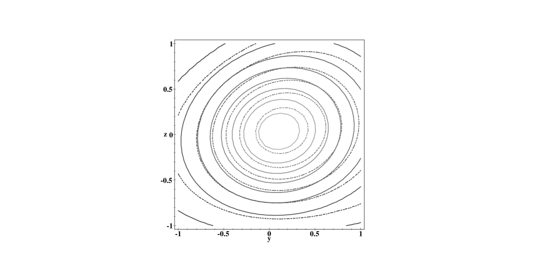
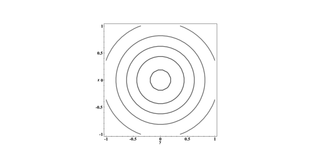
Figure 8: The cross-sections of the volume density at $x=2a/5$ for the $\alpha_{xy}=25^{o}$ and $\alpha_{xy}=50^{o}$ models (solid and dashed contours in the upper panel). The maxima of the contours are where the the long-axis of the bar intersects with the $x=2a/5$ plane. They are offset from the $y=z=0$ point because the long-axis is pointed away from the line of sight. Subtracting one from another we get the phantom spheroidal distribution (lower panel), which has rotational symmetry around the $x$-axis.

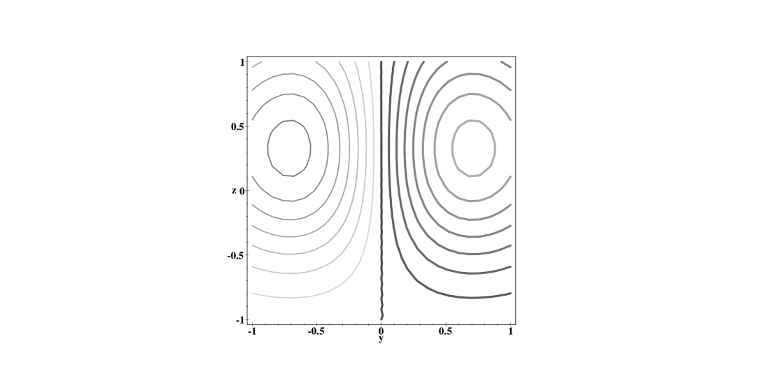
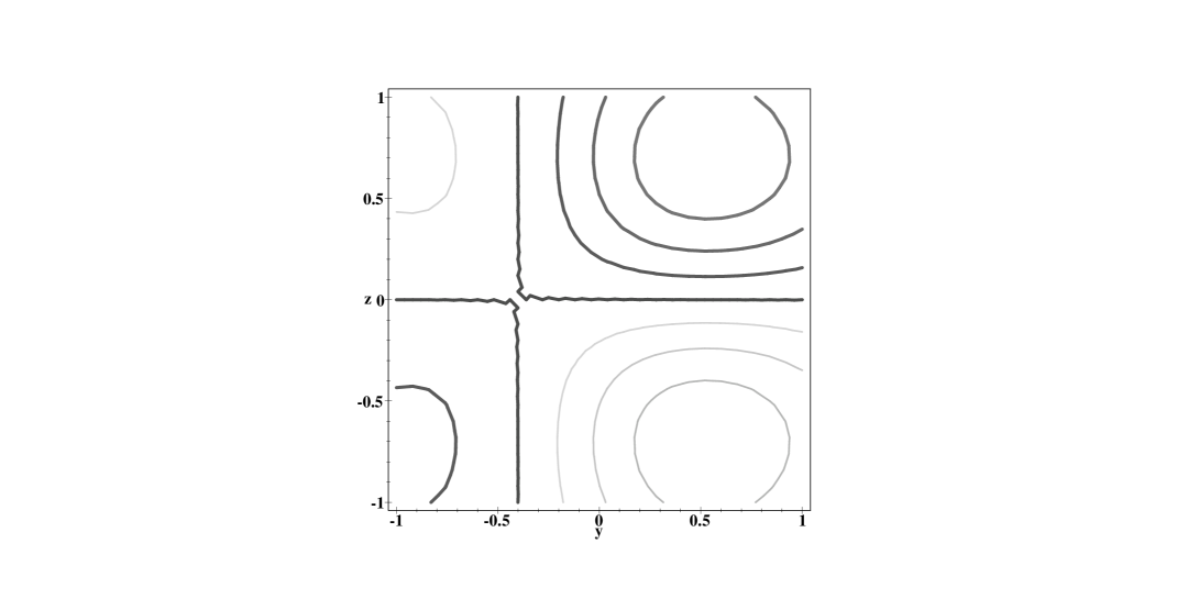
Figure 9: The cross-sections at $x=2a/5$ for the odd part of the model density, which is independent of $\gamma$. The upper panels shows $\nu_{\gamma}(x,y,z)-\nu_{\gamma}(x,-y,z)$, and lower panel shows $\nu_{\gamma}(x,y,z)-\nu_{\gamma}(x,y,-z)$. The distributions are anti-symmetric with respect to the $y=l^{\prime}=0$ plane or the $z=b^{\prime}=0$ plane with both positive (thick contours) and negative contours (thin contours).

The two models differ only in the even part of the volume density as shown by the cross-sections at, say, $x=2a/5$ (cf. Fig. 8). Subtracting one model from another we get back the phantom spheroid, which is rotationally symmetric around the Sun-object center axis.

The odd part of the volume density is identical for both models, and is shown in Fig. (9). Mathematically, the odd part of the density is defined by

$$\nu^{odd,y}\equiv{1\over 2}\left[\nu_{\gamma}(x,y,z)-\nu_{\gamma}(x,-y,z)\right]=2y\left(c_{12}x+c_{23}z\right)p(r),$$ (56)

and

$$\nu^{odd,z}\equiv{1\over 2}\left[\nu_{\gamma}(x,y,z)-\nu_{\gamma}(x,y,-z)\right]=2z\left(c_{13}x+c_{23}y\right)p(r).$$ (57)

Clearly both $\nu^{odd,y}$ and $\nu^{odd,z}$ are independent of $\gamma$, i.e., the amount of PS in the model.

The odd part of the density shows up as the asymmetry in the surface brightness. The left-to-right asymmetry is a line-of-sight integration of $\nu^{odd,y}$ with

$${1\over 2}\left[I(l^{\prime},b^{\prime})-I(-l^{\prime},b^{\prime})\right]=\int_{-\infty}^{\infty}\!\!\nu^{odd,y}dD,$$ (58)

and the up-to-down asymmetry is an integration of $\nu^{odd,z}$ along the line of sight with

$${1\over 2}\left[I(l^{\prime},b^{\prime})-I(l^{\prime},-b^{\prime})\right]=\int_{-\infty}^{\infty}\!\!\nu^{odd,z}dD.$$ (59)

More specific for the Gaussian triaxial models here, the asymmetry along the $b^{\prime}=0$ cut is given by

$${I(l^{\prime},0)-I(-l^{\prime},0)\over 2}=I_{0}\tilde{c}_{12}W(w)\sin 2l^{\prime},~{}~{}~{}\tilde{c}_{12}\equiv{c_{12}\over 2\sqrt{2}+c_{11}},$$ (60)

and the asymmetry along the $l^{\prime}=0$ cut is given by

$${I(0,b^{\prime})-I(0,-b^{\prime})\over 2}=I_{0}\tilde{c}_{13}W(w)\sin 2b^{\prime},~{}~{}~{}\tilde{c}_{13}\equiv{c_{13}\over 2\sqrt{2}+c_{11}}$$ (61)

where $\tilde{c}_{12}$ and $\tilde{c}_{13}$ are the combinations of the intrinsic shape parameters of the model, and

$$W(w)=e^{-{w^{2}\over a^{2}}}\left({2w^{2}\over a^{2}}-1\right),$$ (62)

is a function of the impact parameter $w$. Effectively $W(w)$ is a rescaled asymmetry distribution after removing the periodical anti-symmetric term $\sin 2l^{\prime}$ or $\sin 2b^{\prime}$. Note that the asymmetry distribution has a reversal of sign around the impact parameter

$$w=a/\sqrt{2}.$$ (63)

This means we can derive the scale length of the model $a$ directly from the observable asymmetry map. For example, for the models in Fig. (11), the object is at a distance $D_{0}=4a$, so the reversal of the asymmetry, i.e., $W(w)=0$, happens at

$$|l^{\prime}|=\arcsin{w\over D_{0}}\sim 10^{o},$$ (64)

in the longitudinal cut, or at $|b^{\prime}|\sim 10^{o}$ in the latitudinal cut. While fitting the asymmetry map will tell us unambiguously the scale length $a$ and the shape parameter $\tilde{\epsilon}$ of the triaxial object, it does not directly constrain the major-axis angle $\alpha$, nor does it constrain the amount of phantom spheroidal density.

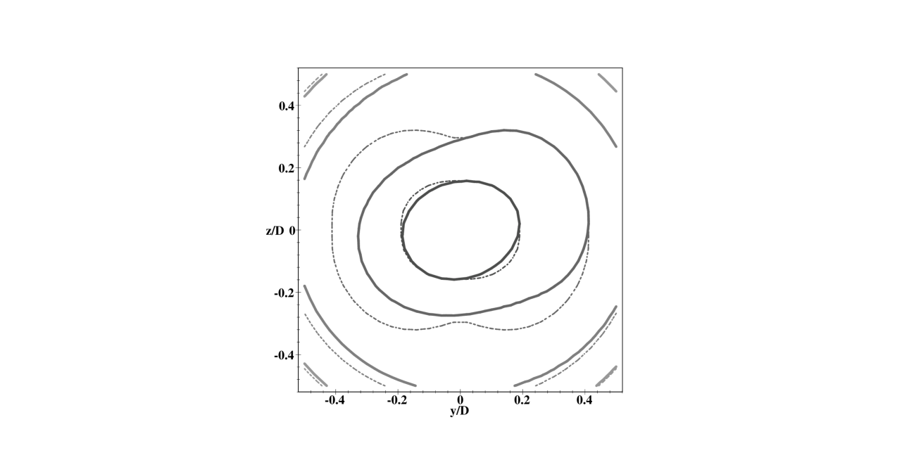
Figure 10: The identical surface brightness map of the two triaxial models from the observer’s perspective, where the horizontal axis $y/D$ and the vertical axis $z/D$ measure the angular distance of a line of sight from the $y=0$ plane and the $z=0$ plane. The dashed contours in the three quadrants are the images of the contours in the first quadrant. The offset with the solid contours shows the asymmetry or the perspective effect of a nearby object. Contours are in intervals of 1 magnitude.

Figure 11: the run of the surface brightness along the $l^{\prime}$-axis (top) and along the $b^{\prime}$-axis (bottom) for our Gaussian triaxial models. The solid curves show symmetric part and the dashed curves show the perspective-induced asymmetry (after blown up by a factor of four). The $l^{\prime}$ and $b^{\prime}$ are the generalized longitude and latitude in units of degrees for the object.

6 Phantom Spheroid vs. the Galactic bar

This new form of non-uniqueness of nearby objects might apply to the Galactic bar as well. As mentioned in the Introduction, the COBE/DIRBE surface brightness distribution is the main source of information about the volume density of the Galactic bar. Imaging the effect of adding any amount of the phantom spheroids here $\gamma F(x,y,z)$ to the COBE bar. It does not matter whether we use the cigar-shaped one in Fig. 1 or the smoother ones shown in Fig. 2, as long as the PS is exactly centered at the Galactic center, i.e., we set $D_{0}$ of these PS densities to the Galactocentric distance (say 8 kpc). The result is a new volume density of the Galaxy with a generally twisted shape in the central part, but there should be no trace of alteration in the the surface brightness maps (the symmetric maps or the asymmetry maps). This is purely because of the construction of the PS (cf. eq. 5). So the perspective effect in the COBE/DIRBE maps is bypassed completely. However, adding any phantom spheroid here will modify only the even part of the volume density and will have no influence on the anti-symmetric part since the PS is always symmetric with respect to the $l=0$ plane and the $b=0$ plane (cf. eq. 6 and Fig. 8). So as illustrated by Fig. (9) and Fig. (10), the prominent perspective effect in the left-to-right asymmetry map $\left[I(l,b)-I(-l,b)\right]/2$ or the up-to-down asymmetry map $\left[I(l,b)-I(l,-b)\right]/2$ should tightly constrain the part of the volume density which is anti-symmetric with respect to the $l=0^{o}$ plane or the $b=0^{o}$ plane (cf. eqs. 58 and 59).

It is tempting to suggest that phantom spheroids are responsible for the uncertain major axis angle of the Galactic bar from the COBE/DIRBE map (Binney & Gerhard 1996, Binney, Gerhard & Spergel 1997). However, this statement depends on whether there exists a phantom spheroidal density which preserves the assumed mirror symmetry of the COBE bar exactly. Unless the added PS has a density profile matching that of the COBE bar, it will create a $m=2$ twist, like a two-armed spiral pattern or an S-shaped warp. On the other hand, part of such distortion may be hidden by the spiral arms in the Galactic disk. After all the mirror symmetry is merely an assumption, which is motivated by the fact that external face-on barred galaxies have a largely bi-symmetric distribution of light. Here we remark that the sequence of Gaussian triaxial models here capture the main features of the Galactic bar and the COBE/DIRBE maps: the models shown in Fig. 6 and 6 with the scalelength $a=D_{0}/4=2$kpc resemble the Gaussian Galactic bar models of Dwek et al. (1995) and Freudenreich (1998) in terms of aspect ratios, radial profile and the offset of the Sun from all three symmetry planes of the bar; the asymmetric patterns in the surface brightness cuts in Fig. (11) also mimics those seen in the COBE/DIRBE maps. Hence it would not be surprising if there exists a phantom spheroid which is qualitatively similar the one prescribed by eq. (45) and preserves the mirror-symmetry of the Galactic bar. Nevertheless a quantitative determination of the parameters of the COBE bar is a complex numerical problem involving to the least a reliable treatment of dust extinction (Arendt et al. 1994, Spergel 1997). Note that patchy dust in the Galaxy makes a phantom spheroid here project to a non-zero irregular surface brightness map. The effect is strongest when the dust is mixed with stars near the center, but even a dust screen near the Sun can cast a faint shadow unless the phantom spheroid is confined inside the solar circle (e.g. the cigar-shaped PS in Fig. 1). The fact that dust extinction is a function of wavelength could constrain the phantom spheroids. The range of the bar angle and axis ratio are also constrained by other observational constraints of the bar such as microlensing optical depth (Zhao & Mao 1996, Bissantz, Englmaier, Binney, & Gerhard 1997) and star counts (Stanek et al. 1994). Star count data, for example, can constrain the line-of-sight distribution of the bar, hence can in principle distinguish between a prolate bar and a spherical bulge, and break the degeneracy of the PS. A detailed numerical treatment of the Galactic bar is beyond the scope of this paper on the existence of non-uniqueness in deprojecting a general nearby object.

7 Phantom Spheroid vs. known non-uniqueness in external galaxies

The phantom spheroidal density for nearby systems is of a different nature from the kind of non-uniqueness associated with a simple shear and/or stretch transformation of an ellipsoid. This applies even in the limit that the object is at infinity because these transformations normally change the odd part of the density, while the PS density here is strictly an even function (cf. eq. 6).

Our phantom spheroidal density $F(x,y,z)$ is a function of the object distance $D_{0}$. In general

$$F(x,y,z)=F_{D_{0}\rightarrow\infty}(x,y,z)+D_{0}^{-2}F_{0}(r),$$ (65)

where $F_{D_{0}\rightarrow\infty}$ is the PS in the limit of $D_{0}\rightarrow\infty$, and $F_{0}(r)$ is (up to a constant) the PS in the limit of $D_{0}\rightarrow 0$. For a hypothetical observer receding from the object, the distance $D_{0}$ increases, the PS density is adjusted slightly to accommodate the changing perspective so to preserve this kind of non-uniqueness all the way to extragalactic distance. The common ambiguity of an extragalactic axisymmetric bulge with an end-on bar is a very special case of the kind of non-uniqueness for nearby objects.

The divergence of $F(x,y,z)$ at small $D_{0}$ (cf. eq. 65) has an interesting implication. In the limit that $D_{0}\rightarrow 0$ some regions of the phantom spheroid will have infinitely positive density, and some regions infinitely negative density because $\gamma F(x,y,z)\rightarrow\gamma D_{0}^{-2}F_{0}(r)$, and $F_{0}(r)$ changes sign, for example, at $r=a\sqrt{3/2}$ (cf. eq. 45 or Fig. 4). So to add any finite amount of PS would violate the positivity requirement. Hence only the model with $\gamma=0$ is allowed, and the major axis direction is fixed to the direction where the object appears the brightest in the projected map. In other words the kind of non-uniqueness discussed here disappears if the observer is very close to the object center. In general the range for $\gamma$ becomes very narrow if $D_{0}\leq a$, and is insensitive to the distance $D_{0}$ to the object if $D_{0}>2a$.

Unlike its external counterpart with $D_{0}\rightarrow\infty$, the PS density for a nearby triaxial body is not massless. The total luminosity $L_{\gamma}$ of our model changes with $\gamma$. For the Gaussian model we have (cf. eqs. 30 and 48)

$$L_{\gamma} = \int\!\!d^{3}{\bf r}\nu_{\gamma}(x,y,z)=L_{0}+\gamma L_{PS},$$ (66)

$$L_{0} = \pi^{3\over 2}\nu_{c}a^{3}\left[2^{3\over 2}+{c_{11}+c_{22}+c_{33}\over 2}\right],$$

$$L_{PS} = -\left({3\pi^{3\over 2}\nu_{c}a^{3}\over 2}\right)\left({\gamma a^{2}\over D_{0}^{2}}\right),$$

where $L_{0}$ is the luminosity in the absence of the PS. The PS has a luminosity $L_{PS}$ proportional to $D_{0}^{-2}$.

The normalization $\nu_{c}$ and the scale $a$ are fixed by the projected light intensity $I_{0}$ and the asymmetry map $W(w)$ (cf. eqs. 62 and 39), but the total luminosity changes by a fraction of the order of ${a^{2}\over D_{0}^{2}}$. This is because unlike external systems, the observed angular distribution of light in a nearby object does not simply sum up to a unique measurement of its total luminosity. We may slightly underestimate/overestimate the intrinsic luminosity by about a few percent, which may not be easy to detect in reality. Moving away from the object the observer has a full outside view and hence a better determination of its luminosity but at the expense of relaxing the constraint on the orientation of the object from the perspective effect and positivity.

The phantom spheroid affects also the dynamics of the model, however, the effect can be fairly difficult to detect. For the models in eq. (23), the depth of the potential well at the center expressed in terms of the escape velocity $V_{esc}$ is given by

$${1\over 2}V_{esc}^{2}=\pi\nu_{c}a^{2}G(M/L)\left\{\left[4+{2\over 3}\left(c_{11}+c_{22}+c_{33}\right)\right]-\left({1\over 3}+{a^{2}\over D_{0}^{2}}\right)\gamma\right\},$$ (67)

which decreases linearly with increasing fraction ($\gamma$) of the superimposed PS, where $M/L$ is the mass-to-light ratio. As a result, the potential well of the $\alpha=25^{o}$ model is slightly shallower than that of the more centrally concentrated $\alpha=50^{o}$ model (cf. Fig. 6 and 6). However, the difference is only 7% in terms of the maximum escape velocity $V_{esc}$ of the models. The differences in terms of the mass weighted average velocity dispersion (estimated from the virial theorem) and the circular velocity (estimated directly from the potential) are also at only a few percent level, too small to be measured with certainty. However it might still be feasible to distinguish the models in terms of the stellar orbits in them. The projected velocity distribution should change with the major axis angle.

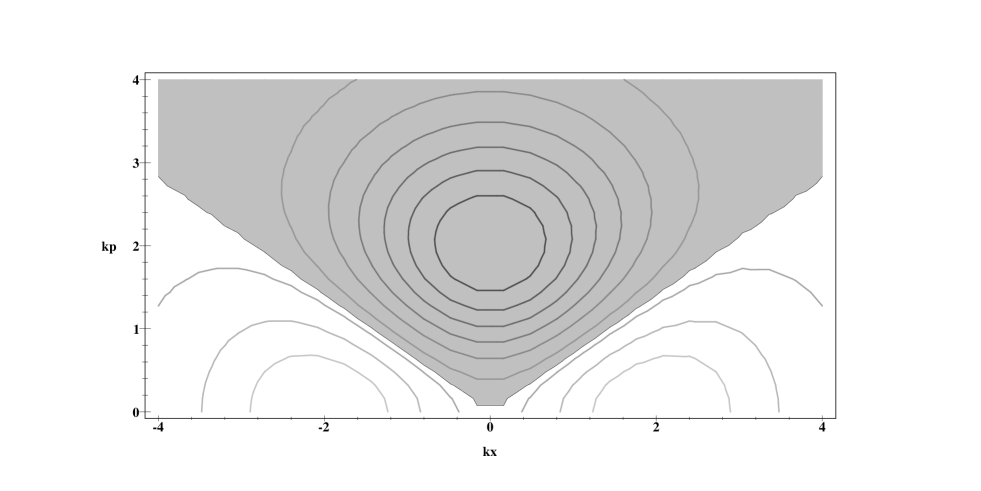
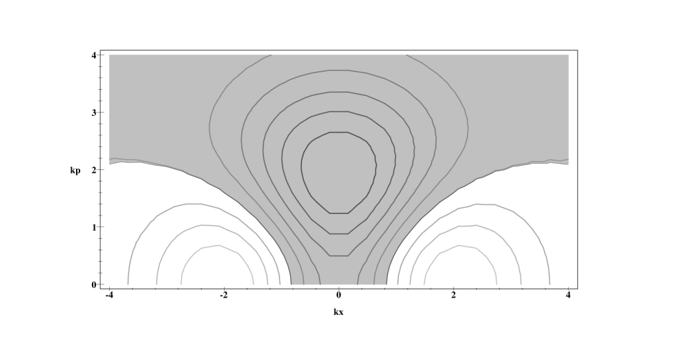
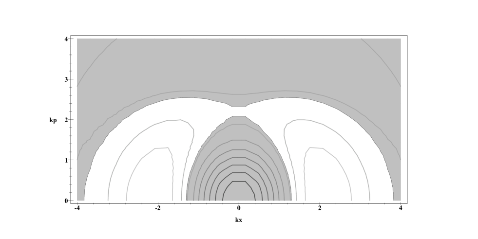
Figure 12: The phantom density in the Fourier ${\bf k}$-space, $k_{x}$ vs. $k_{p}=\sqrt{k_{y}^{2}+k_{z}^{2}}$ in units of $a^{-1}$. The distributions are rotationally symmetric around the $k_{x}$-axis. The shaded and unshaded zones correspond to negative and positive $\tilde{F}({\bf k})$ respectively. The observer is at $D_{0}=\infty,4a,1.25a$ from top to bottom.

Our phantom spheroidal density is also different from konuses since it is not confined to any cone in the Fourier k-space even in the limit $D_{0}\rightarrow\infty$. Using eqs. (4), (24) and (25) of Palmer (1994) we can compute the Fourier transform of our PS (cf. eq. 45). We find

$$\tilde{F}({\bf k})\equiv\int\!\!d^{3}{\bf r}\exp(-i{\bf k}\cdot{\bf r})\left[p(r)x^{2}-S(r)\right]=\tilde{F}_{D_{0}\rightarrow\infty}({\bf k})+D_{0}^{-2}\tilde{F}_{0}({\bf k}),$$ (68)

which is a k-space spheroidal distribution around the Sun-center line, where

$$\tilde{F}_{D_{0}\rightarrow\infty}({\bf k})\equiv\pi^{3\over 2}\nu_{c}a^{3}\left(\cos^{2}\theta_{{\bf k}}-{2\over 3}\right){k^{2}a^{2}\over 4}e^{-{k^{2}a^{2}\over 4}},$$ (69)

$\theta_{{\bf k}}$ is the angle of the k-vector with the Sun-center line, and

$$D_{0}^{-2}\tilde{F}_{0}({\bf k})\equiv\left(1-{7k^{2}a^{2}\over 12}+{k^{4}a^{4}\over 24}\right)e^{-{k^{2}a^{2}\over 4}}L_{PS}.$$ (70)

We recover the luminosity of the PS in the limit ${\bf k}\rightarrow 0$, $\tilde{F}(0)=D_{0}^{-2}\tilde{F}_{0}(0)=L_{PS}$ (cf. eq. 66). Fig. 12 shows that even when the object is placed at infinity, $\tilde{F}({\bf k})$ is non-zero everywhere except at k$=0$ or $\theta_{{\bf k}}=\cos^{-1}\sqrt{2\over 3}$ (cf. eq. 69). Since any konus-like structure (or its triaxial version) must have a certain “cone of ignorance” around a principal axis of the model outside which $\tilde{F}({\bf k})=0$ (Rybicki 1986, Gerhard & Binney 1996, Kochanek & Rybicki 1996), the kind of non-uniqueness shown in this paper has little to do with konuses. The two sequences of models meet only when the object is a face-on or end-on spheroidal system, in which case, the PS here is equivalent to a trivial konus with the entire ${\bf k}$-space in the “cone of ignorance”.

8 Conclusion

The non-uniqueness in deprojecting the surface brightness maps of a nearby system can originate from the simple fact that a spherical bulge can match an end-on prolate bar or a face-on disk in the line-of-sight integrated light distribution. Subtracting the spherical bulge from the prolate end-on bar or the face-on disk forms a phantom spheroid (PS), which has both positive and negative density regions. The non-uniqueness due to such PS can be characterized by two numbers: the distance ($D_{0}$) of the object and the amount ($\gamma$) of the PS density that we can superimpose. By tailoring the PS, it is possible to preserve the triaxial reflection symmetries of the model. The orientation of these symmetry planes with respect to our line of sight changes as increasing amount of PS is added up to the point when negative density regions appear in the final model. The limits on the major-axis angles are given analytically. The phantom spheroidal density here forms a new class of non-uniqueness of entirely different nature from known degeneracy in deprojecting extragalactic objects. It does not preserve the total luminosity of the system.

The author thanks Frank van den Bosch and Tim de Zeeuw for many helpful comments on the presentation, and Ortwin Gerhard for careful reading of an early draft.

Appendix A Positivity as a constraint to the major axis angle of edge-on models

Edge-on models are specified by

$$c_{23}=c_{31}=\alpha_{yz}=\alpha_{xz}=0,~{}~{}~{}c_{12}\equiv\epsilon,~{}~{}~{}\alpha\equiv\alpha_{xy},$$ (71)

so that the $z=0$ plane, which passes through the observer at $(x,y,z)=(D_{0},0,0)$, is a symmetry plane of the model. The volume density model of the system is best described in a cylindrical coordinate system $(R,Z,\psi)$ centered on the object. This coordinate system is related to the rectangular coordinate system by

$$x=R\cos\psi,~{}~{}~{}y=R\sin\psi,~{}~{}~{}z=Z,$$ (72)

where the $Z$-axis is the symmetry axis of the edge-on system, and $\psi=0$ is a plane, passing through the Sun-object line and the $Z$-axis. In this coordinate system we can rewrite the ellipsoidal term $Q_{\gamma}$ (cf. eq. 26) as

$$Q_{\gamma}=\left[c_{33}Z^{2}+\left(c_{22}+\epsilon\cot 2\alpha\right)R^{2}\right]+{\epsilon R^{2}\over\sin 2\alpha}\cos(2\psi-2\alpha).$$ (73)

Clearly surfaces of constant $Q_{\gamma}$ are ellipsoidal surfaces with mirror symmetry with respect to the $\psi=\alpha$ plane, the $\psi=\alpha+{\pi\over 2}$ plane and the $Z=0$ plane.

The triaxial model density (cf. eq. 24) can then be written in above notations as

$$\nu_{\gamma}(R,Z,\psi)=n_{0}(R,Z)+n_{2}(R,Z)\cos(2\psi-2\alpha),$$ (74)

where the second term is a triaxial perturbation with the major axis along $\psi=\alpha$ and amplitude

$$n_{2}(R,Z)={\epsilon R^{2}p\over\sin 2\alpha},$$ (75)

and the first term, the axisymmetric part, is given by

$$n_{0}(R,Z)\equiv E(R,Z)+\epsilon\cot 2\alpha\left[R^{2}p-2S\right],$$ (76)

where

$$E(R,Z)\equiv\left[G+(c_{11}-c_{22})S\right]+(c_{22}R^{2}+c_{33}Z^{2})p.$$ (77)

Imposing positivity requirements to $\nu_{\gamma}(R,Z,\psi)$ for all values of the azimuthal angle $\psi$, we have

$$n_{0}(R,Z)\geq n_{2}(R,Z),$$ (78)

i.e.,

$$E(R,Z)+\epsilon\cot 2\alpha\left[R^{2}p-2S\right]\geq{\epsilon R^{2}p\over\sin 2\alpha}.$$ (79)

Using the following relations for sinusoidal functions

$${1\over\sin 2\alpha}={1+t^{2}\over 2t},~{}~{}\cot 2\alpha={1-t^{2}\over 2t},~{}~{}t\equiv\tan\alpha,$$ (80)

the inequality reduces to an upper and a lower bound for the angle $\alpha$ with,

$$\rm Max\left[t_{-}\right]\leq\tan\alpha\leq\rm Min\left[t_{+}\right],$$ (81)

where $t_{-}\leq t\leq t_{+}$ is the range bounded by the effectively quadratic inequality for $t$

$$\left[\epsilon R^{2}p-\epsilon S\right]t+\epsilon St^{-1}\leq E(R,Z)$$ (82)

at a given position $(R,Z)$ on the meridional plane, and the overlapped interval of these ranges is used in eq. (81). For example, for models with parameters in eq. (40) and $D_{0}=4a$, we find $77^{o}>\alpha>15^{o}$ to ensure a positive density at $(R,Z)=(a,a)$, but a narrower range $63.5^{o}\geq\alpha\geq 22.5^{o}$ is necessary to ensure positivity everywhere in the $(R,Z)$ plane.

Interestingly we recover the results of eq. (34) if we integrate both sides of eq. (82) along the $y$-axis. And likewise if we multiply both sides of eq. (82) by a factor $x^{2}$ and then integrate along the $x$-axis, we recover the results of eq. (37).

Appendix B Analytical expressions for a series of phantom spheroids

New phantom spheroids can be generated from the original PS $F(x,y,z)=x^{2}p(r)-S(r)$ (cf. eq. 45) by repeatedly applying the derivative operator ${1\over 2}{\partial\over\partial\ln a}$, i.e,

$$F_{1}(x,y,z)={\partial F(x,y,z)\over 2\partial(\ln a)}=x^{2}p_{1}(r)-S_{1}(r),$$ (83)

where

$$p_{1}(r)\equiv{\partial p(r)\over 2\partial(\ln a)}=-p(r)\left(1-{r^{2}\over a^{2}}\right),$$ (84)

$$S_{1}(r)\equiv{\partial S(r)\over 2\partial(\ln a)}=a^{2}p(r)\left[{r^{2}\over 2a^{2}}+{a^{2}\over D_{0}^{2}}\left(-{5r^{4}\over 2a^{4}}+{r^{6}\over a^{6}}\right)\right],$$ (85)

and

$$F_{2}(x,y,z)={\partial F_{1}(x,y,z)\over 2\partial(\ln a)}=x^{2}p_{2}(r)-S_{2}(r),$$ (86)

where

$$p_{2}(r)\equiv{\partial p_{1}(r)\over 2\partial(\ln a)}=p(r)\left(1-{3r^{2}\over a^{2}}+{r^{4}\over a^{4}}\right),$$ (87)

$$S_{2}(r)\equiv{\partial S_{1}(r)\over 2\partial(\ln a)}=-a^{2}p(r)\left[\left({r^{2}\over 2a^{2}}-{r^{4}\over 2a^{4}}\right)+{a^{2}\over D_{0}^{2}}\left(-{5r^{4}\over 2a^{4}}+{9r^{6}\over a^{6}}-{r^{8}\over a^{8}}\right)\right].$$ (88)

References

- [1] Arendt R.G. et al., 1994, ApJ, 425, L85
- [2] Binney, J.J., & Tremaine, S., 1987, Galactic Dynamics (Princeton: Princeton Univ.).
- [3] Binney J.J., & Gerhard O.E., 1996, MNRAS, 279, 1005
- [4] Binney J.J., & Gerhard O.E., & Spergel D.N. 1997, MNRAS, 288, 365
- [5] Bissantz N., Englmaier P., Binney J.J., Gerhard O. 1997, MNRAS, 289, 651 (astro-ph/9612026).
- [6] Blitz L. & Spergel D.N. 1991, ApJ, 379, 631.
- [7] Contopoulos G. 1956, Z. Astrophys., 39, 126
- [8] Dwek E. et al. 1995, ApJ 445, 716
- [9] Freudenreich, H.T. 1998, ApJ, 492, 495
- [10] Gerhard O.E. & Binney J.J., 1996, MNRAS 279, 993
- [11] Kochanek C.S. & Rybicki G.B. 1996, MNRAS, 280, 1257
- [12] Palmer P.L. 1994, MNRAS, 266, 697
- [13] Romanowsky A.J., Kochanek C.S. 1997, MNRAS, 287, 35 (astro-ph/9609202)
- [14] Rybicki G.B. 1986, in Structures and dynamics of elliptical galaxies, IAU Symp. 127, ed. de Zeeuw P.T., Kluwer, Dordrecht, 397
- [15] Spergel D.N. 1997, private communication
- [16] Stanek K.Z., Mateo M., Udalski, A., Szymański, M., Kaluźny, J., Kubiak, M. 1994, Ap.J., 429, L73
- [17] van den Bosch F.C. 1997, MNRAS, 287, 543
- [18] Weiland J. et al. 1994, ApJ, 425, L81.
- [19] Zhao H.S. & Mao S. 1996, MNRAS, 283, 1197