The RASSCALS: An X-ray and Optical Study of 260 Galaxy Groups

Abstract

We describe the ROSAT All-Sky Survey—Center for Astrophysics Loose Systems (RASSCALS), the largest X-ray and optical survey of low mass galaxy groups to date. We draw 260 groups from the combined Center for Astrophysics and Southern Sky Redshift Surveys, covering one quarter of the sky to a limiting Zwicky magnitude of $m_{z}=15.5$. We detect 61 groups (23%) as extended X-ray sources.

The statistical completeness of the sample allows us to make the first measurement of the X-ray selection function of groups, along with a clean determination of their fundamental scaling laws. We find robust evidence of similarity breaking in the relationship between the X-ray luminosity and velocity dispersion. Groups with $\sigma_{p}<340$ km s^-1 are overluminous by several orders of magnitude compared to the familiar $L_{X}\propto\sigma^{4}$ law for higher velocity dispersion systems. An understanding of this break depends on the detailed structure of groups with small velocity dispersions $\sigma_{p}<150$ km s^-1.

After accounting for selection effects, we conclude that only 40% of the optical groups are extended X-ray sources. The remaining 60% are either accidental superpositions, or systems devoid of X-ray emitting gas. Combining our results with group statistics from N-body simulations, we find that the fraction of real, bound systems in our objectively selected optical catalog is between 40%–80%.

The X-ray detections have a median membership of 9 galaxies, a median recession velocity $cz=7250$ km s^-1, a median projected velocity dispersion $\sigma_{p}=400$ km s^-1, and a median X-ray luminosity $L_{X}=3\times 10^{42}h_{100}^{-2}$ erg s^-1, where the Hubble constant is $H_{0}=100h_{100}$ km s^-1 Mpc^-1. We include a catalog of these properties, or the appropriate upper limits, for all 260 groups.

1. Introduction

The ROSAT and ASCA missions have shown that even low mass systems of galaxies contain a hot intergalactic plasma. Many of the Hickson (1982) compact groups (HCGs) are embedded in diffuse X-ray emission detectable by the ROSAT (Ebeling, Voges, & Böhringer 1994; Pildis, Bregman, & Evrard 1995; Ponman et al. 1996). Other ROSAT studies of smaller group samples (e.g. Henry et al. 1995; Burns et al. 1996; Mulchaey et al. 1996; Mahdavi et al. 1997; Mulchaey & Zabludoff 1998) confirm the existence of an intergalactic plasma with an average temperature $kT\approx 1$ keV in many loose groups.

Although heterogeneous studies abound, an objective survey of the nearby universe for X-ray emitting groups is lacking. A search based on a large optical catalog, drawn objectively from a three dimensional map of the large scale structure, is essential for understanding the physical properties of galaxy groups. Here we construct the first such catalog. Our goals are (1) to investigate similarity breaking in the fundamental scaling laws of systems of galaxies, (2) to make the first calculation of the X-ray selection function of galaxy groups, and (3) to place firm limits on the fraction of optically selected groups that are bound.

One important example of similarity breaking is the relationship between the X-ray luminosity $L_{X}$ and the average plasma temperature $T$. Ponman et al. (1996) show that the $L_{X}-T$ relation is quite steep for compact groups, with $L_{X}\propto T^{5}$, whereas for rich clusters $L_{X}\propto T^{3}$. This result is consistent with a “preheating” scenario where winds from supernovae in galaxies undergoing the starburst phase leave their mark on the poorest systems. Such winds would deplete the intragroup plasma (Davis, Mulchaey, & Mushotzky 1999; Hwang et al. 1999), raise the gas entropy relative to the gravitational collapse value (Ponman, Cannon, & Navarro 1999), and preferentially dim the systems with the lowest temperatures (Cavaliere, Menci, & Tozzi 1997).

Systems in hydrostatic equilibrium should have $T\propto\sigma_{p}^{2}$, where $\sigma_{p}$ is the velocity dispersion of the dark matter halo in which the galaxies are embedded. Thus one might expect that the $L_{X}-\sigma_{p}$ and the $L_{X}-T$ relations for groups of galaxies steepen in a similar manner. Here we show that quite the opposite is true. The groups with the smallest velocity dispersions are in fact overluminous compared to the $L_{X}\propto\sigma^{4}$ law valid for higher velocity dispersion systems. Thus the similarity breaking in the $L_{X}-T$ law is apparently incommensurate with the break in the $L_{X}-\sigma_{p}$ relation. We discuss several plausible explanations for this lack of concordance.

The paper is organized as follows. After constructing the catalog (§2), we examine the $L_{X}-\sigma_{p}$ relation (§3), calculate the selection function (§4), discuss the $L_{X}-\sigma_{p}$ flattening (§5), and summarize our findings (§6). We call our groups the ROSAT All-Sky Survey—Center for Astrophysics Loose Systems, or RASSCALS.

2. Data

2.1. Optical Group Selection

We extract the optical group catalog for the RASSCALS study from two complete redshift surveys. Our catalog includes a wide variety of systems, from groups with only $5$ members to the Coma cluster .

The Center For Astrophysics Redshift Survey (Geller & Huchra 1989; Huchra et al. 1990; Huchra, Geller, & Corwin 1995; CfA) and the Southern Sky Redshift Survey (Da Costa et al. 1994; Da Costa et al. 1998), both complete to a limiting Zwicky magnitude $m_{z}\approx 15.5$, serve as sources for the RASSCALS. The portion of the surveys we use covers one fourth of the sky in separate sections described in Table 1. We transform the redshifts to the Local Group frame ($\Delta cz=300\sin{l}\cos{b}$), and correct them for infall toward the center of the Virgo cluster (300 km s^-1 towards $\alpha_{2000}=12^{\mathrm{h}}31.2\mathrm{m}$, $\delta_{2000}=12$°2.54^′).

We use the two-parameter friends-of-friends algorithm (FOFA) to construct the optical catalog. Huchra & Geller (1982) first described the FOFA for use with redshift surveys, and Ramella, Pisani, & Geller (1997) applied it to the NRG data. The FOFA is a three-dimensional algorithm which identifies regions with a galaxy overdensity $\delta\rho/\rho$ greater than some specified threshold. A second fiducial parameter, $V_{0}$, rejects galaxies in the overdense region which are too far removed in velocity space from their nearest neighbor. The N-body simulations of Frederic (1995) and Diaferio (1999) show that the Huchra & Geller (1982) detection method misses few real systems, at the cost of including some spurious ones. We apply the FOFA to the combined NRG, SRG, and SS2 redshift surveys with $\delta\rho/\rho=80.$

The RASSCALS optical catalog contains 260 systems with $n\geq 5$ members and 3000 km s^-1$\leq cz\leq 12000$ km s^-1. The low velocity cutoff rejects systems that cover a large area on the sky and thus may be affected by the Local Supercluster. The median recession velocity for the systems is 7000 km s^-1; the effects of cosmology and evolution are negligible throughout the sample. Table 2 lists the individual groups and their properties. Figures 1–2 show the sky positions of the member galaxies for the systems with statistically significant extended X-ray emission in the RASS.

To compare the membership of groups which have different redshifts we also compute $n_{17}$, the number of group members brighter than an absolute magnitude $M_{z}=-17$, corresponding to $m_{z}=15.5$ for a group at $cz=3200$ km s^-1. To calculate $n_{17}$, we assume that the galaxies in groups have the same luminosity function as the Center for Astrophysics Redshift Survey (Marzke et al. 1994), reconvolved with the magnitude errors. The resulting distribution is well-represented by a Schechter (1976) function with a characteristic absolute magnitude $M_{*}=-19.1$ and a faint-end slope $\alpha=-1$. Table 2 lists $n_{17}$, which has a median value of 44.

2.2. X-Ray Field Selection

For every system in the RASSCALS optical catalog, we obtain X-ray data from a newly processed version of the ROSAT All-Sky Survey (Voges et al. 1999), which corrects effects leading to a low detection rate in the original reduction.

We first assign each system a seven-character name, beginning with “NRG,” “SRG,” or “SS2,” followed by “b” or “s” (specifying the angular size of the system as “big,” with $cz<8500$ km s^-1 or “small,” with $cz>8500$ km s^-1, respectively), followed by a three-digit number.

For each “small” system we extract a square field measuring $2^{\circ}\times 2^{\circ}$ from the RASS; for the “big” systems we extract a $3.5^{\circ}\times 3.5^{\circ}$ square. The fields are centered at the mean RA and DEC of the galaxies; every field is at least large enough to include a circle with a projected radius of $1h_{100}^{-1}$ Mpc around the optical center of the system it contains. We use photons in the 0.5–2.0 keV hard energy band of the Position-Sensitive Proportional Counter (PSPC channels 52-201).

2.3. Detection Algorithm

The X-ray detection algorithm consists of four steps: measurement of the background, source identification, decontamination, and measurement of the source flux.

We determine the mean background by temporarily rebinning the exposure-weighted ROSAT field into an image with $15\arcmin$ pixels. We clean the image of all fluctuations with an iterative, $2.5\sigma$ clipping algorithm. The adopted background is then the average of the remaining pixel values.

To estimate the probability that a given group is an X-ray source, we use an optical galaxy position template (GPT). Mahdavi et al. (1997), who search the RASS for X-ray emission from a small subset of our sample, describe this method in greater detail. The GPT is defined as the union of all projected $d=0.2h_{100}^{-1}$ Mpc regions around the group members, excluding any galaxies isolated by more than $d$ from the rest of the group. We count the X-ray photons within the GPT and evaluate the probability that they are drawn from the background distribution. All groups that have a detection significance greater than $2.5\sigma$ progress to the next step.

We identify the emission peak which coincides most closely with the optical center of the group as its X-ray counterpart, and calculate the X-ray position of the group with the intensity-weighted first moment of the pixel values. Using standard maximum likelihood techniques, we identify contaminating X-ray point sources over the entire field. We remove these sources by excising a ring of radius 3$\arcmin$, roughly three times the full width at half maximum of the ROSAT PSPC point spread function (PSF). Unrelated extended sources often contaminate the group emission; we use a suitably larger aperture to remove them. We have examined publicly available ROSAT High-Resolution Imager (HRI) observations of a few groups, and find that our RASS decontamination procedure is satisfactory.

To reject groups with entirely pointlike X-ray emission, we calculate $N(R)$, the cumulative distribution of the ROSAT counts. We use use the Kolmogorov-Smirnov (KS) Test to compare the shape of the emission peak with that of the PSPC PSF combined with the background. We take sources with $P_{\mathrm{KS}}\leq 0.05$ as inconsistent with the PSF.

Finally, we convert the PSPC count rate into $L_{X}(R)$, the 0.1–2.4 keV X-ray luminosity contained within a ring of projected radius $R$. The Appendix describes the flux conversion procedure in detail.

Properties of the NOCORE estimator: (a) $\xi(R)$ for $\beta$-models with $\beta=0.65$ (solid line) and $\beta=1$ (dashed line); (b) $R_{\xi}$, the radius where $\xi(R)$ is minimum, as a function of $\beta$.

2.4. Core Radius Estimation

Here we describe a procedure for identifying a physical scale for the X-ray emission. There is a great deal of evidence that the emissivity profiles of clusters of galaxies exhibit a characteristic scale, or core radius, $r_{c}$ (e.g. Jones & Forman 1984; Mohr, Mathiesen, & Evrard 1999). For example, the “$\beta$-model” emissivity profile frequently used to fit observations of dynamically relaxed systems,

$$\epsilon(r)\propto\left(1+\frac{r^{2}}{r_{c}^{2}}\right)^{-3\beta},$$ (1)

is nearly constant for physical radii $r\ll r_{c}$, and scales as $r^{-6\beta}$ for $r\gg r_{c}$. There is also evidence for cuspy profiles ($\epsilon\propto r^{-1}$ for $r\ll r_{c}$) in clusters with cooling flows (Thomas 1998).

The usual method for measuring $r_{c}$ from X-ray observations consists of projecting $\epsilon(r)$ along one dimension, and fitting the resulting surface brightness profile to the data. This approach has the disadvantage that the resulting estimate of $r_{c}$ is model-dependent, and is often strongly correlated with the slope parameter $\beta$, even with very high quality data (e.g. Jones & Forman 1984; Neumann & Arnaud 1999). Furthermore, its application to the RASSCALS is limited, because the small number of counts and the relatively large uncertainty in the background make it difficult to reconstruct accurate surface brightness profiles for all but the brightest systems.

We therefore use the Nonparametric Core Radius Estimator (NOCORE; Mahdavi 2000) to avoid the core fitting procedure and its associated uncertainties. NOCORE is model-independent; it does not require an estimation of the background, and it relies on the properties of the integrated emission profile, rather than the differential profile, to estimate the core radius. Its only assumption is the constancy of the background level at the position of the object of interest.

Now we outline the procedure. Consider the measured count rate within an annulus $R$ from the X-ray center of the group: it consists of the emission of the group itself, $S(R)$, plus the constant background count rate per unit area, $B$:

$$N(R)=S(R)+\pi R^{2}B.$$ (2)

The fundamental basis of NOCORE is the observation that the quantity $N(R)-k^{2}N(R/k)$, where $k$ is a number greater than 1, is completely independent of the constant background. Formally, we define the NOCORE radius as the radius where the function

$$\xi(R)\equiv\frac{N(R)-4N(R/2)}{R}$$ (3)

has a global minimum. The division by $R$ is necessary to obtain a detectable minimum.

Figure 2.3a shows $\xi(R)$ for theoretical $\beta$-models with $\beta=0.65$ and $\beta=1$. The minimum, $R_{\xi}$, is well-defined in both cases. The location of $R_{\xi}$ as a function of $\beta$ appears in Figure 2.3b. We have carried out numerical tests of the method, adding Poisson noise and a background to a variety of $\beta$-models, to verify that we recover the appropriate core radius without bias. When applying the method to the observations, we use bootstrap resampling to determine 68% confidence intervals on $R_{\xi}$.

As long as there is a characteristic scale in the emissivity profile of a system, NOCORE will find it. The function $\xi(R)$ has a well-defined minimum even in cases when the $\beta$-model is not a good description of the emissivity, for example systems with a cooling flow. If there is more than one characteristic scale in the profile—if the emissivity has features at several radii, because of substructure in the cluster, for example—then $\xi(R)$ has more than one minimum. If the profile is a pure power law, NOCORE shows no core; $\xi(R)$ is then a monotonically decreasing or increasing function of $R$.

We use the radius at which $\xi(R)$ is minimum as a measure of the physical scale of the X-ray emission.

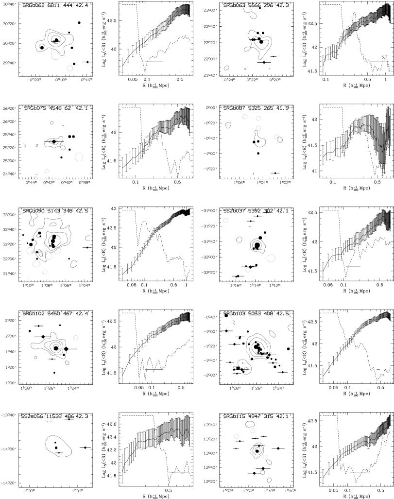
Figure 1.— The RASSCALS. Sky maps are 1.5$h_{100}^{-1}$ Mpc wide, and include the name of each group, its mean recession velocity, velocity dispersion, and log X-Ray luminosity within 0.5$h_{100}^{-1}$ Mpc. The solid X-ray emission contours begin at 1$\sigma$ above the background and increase by a factor of 2. Dotted regions represent sources excised by the decontamination algorithm. Circles represent early-type galaxies, and the elongated symbols represent late-type galaxies. The size of the symbols is proportional to their apparent Zwicky magnitude; the largest symbol corresponds to $m_{Z}=12$, and the smallest corresponds to $m_{Z}=15.5$. Also shown are the background-subtracted cumulative X-ray luminosity profile, and the NOCORE estimator $\xi(R)$. The 68% confidence interval of the NOCORE radius $R_{\xi}$ appears as a horizontal bar.

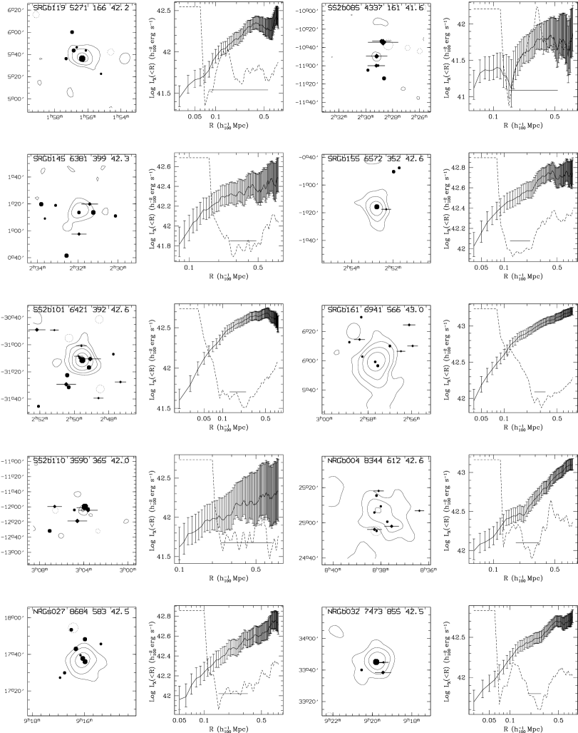
Figure 2.— See caption for Figure 1. Figures for the remainder of the X-ray detected RASSCALS will appear in the published version of this article, in The Astrophysical Journal.

2.5. General Properties of the Final Catalog

Table 3 lists the projected velocity dispersion, $\sigma_{p}$, the 0.1–2.4 keV X-ray luminosity, and the NOCORE radius $R_{\xi}$ of the detected groups. There are 61 detections, of which two (NRGs372 and NRGs392) are bright X-ray clusters (Abell 2147 and 2199) that the friends-of-friends algorithm has broken up into pieces. We count these clusters as detections but we do not calculate luminosities for them. Figures 1–2 show galaxy positions and X-ray emission contours for the detected groups.

Because the diffuse X-ray emission is generally a marker of gas held in a gravitational potential, these systems are probably bound configurations. There is, however, a chance that the X-ray emission might be due to projection along an unbound filament in the large scale structure of the universe (Hernquist, Katz, & Weinberg 1995). The galaxies projected along this line of sight might also have similar redshifts without being bound. However, deeper redshift surveys in the fields of X-ray emitting RASSCALS show that a number of these systems have velocity dispersion profiles $\sigma_{p}(R)$ that decline as a function of projected distance from the group center; these profiles are consistent with the expectation for a relaxed dynamical system (Mahdavi et al. 1999).

In Figures 1–2 we also show the cumulative luminosity profile and the NOCORE estimator $\xi(R)$. In several cases $\xi(R)$ appears to have several local minima in addition to the global minimum. The local minima are almost always due to Poisson noise and deviations from spherical symmetry in the structure of the gas. The confidence intervals on $R_{\xi}$ take these fluctuations into account: when the fluctuations in $\xi(R)$ dominate its shape, the error in $R_{\xi}$ is large. But when $\xi(R)$ has a well-defined global minimum and the fluctuations are small, $R_{\xi}$ is relatively well determined.

3. $L_{X}-\sigma_{p}$ Relation

Here we examine the relationship between the X-ray luminosity and the projected velocity dispersion. First we comment on the link between the $L_{X}-\sigma_{p}$ scaling law, which relates X-ray and optical data, and the $L_{X}-T$ scaling law, which is internal to X-ray data. Then we describe the actual relation.

3.1. Background on the Scaling Laws

If the member galaxies trace the total mass distribution in a cluster, a simple theoretical calculation (Quintana & Melnick 1982) predicts that a spherically symmetric ball of gas should have $L_{X}\propto f^{2}\sigma_{p}^{3}T^{1/2}$, where $f$ is the ratio of the gas mass to the total mass. A further, common assumption is that $T\propto\sigma_{p}^{2}$, i.e., that the emission-weighted gas temperature is proportional to the depth of the gravitational potential. These assumptions yield $L_{X}\propto f^{2}T^{2}\propto f^{2}\sigma^{4}$.

The observed $L_{X}-\sigma_{p}$ relation for rich clusters is in good agreement with the theoretical prediction; Quintana & Melnick (1982) and Mulchaey & Zabludoff (1998), for example, find slopes consistent with $L_{X}\propto\sigma^{4}$. The empirical $L_{X}-T$, relation, however, is somewhat steeper than expected, with most finding $L_{X}\propto T^{2.75}$, even after removing the central cooling flow region (e.g., Markevitch 1998 and references therein).

If the discrepancy between the simple theoretical prediction, $L_{X}\propto T^{2}$, and the observations is real, several effects might explain it. It could be that $f$ increases slightly with $T$ (David, Jones, & Forman 1995), or that $T\propto\sigma^{1.5}$, consistent with a nonisothermal, polytropic gas distribution (Wu, Fan, & Xu 1998). Finally, preheating of gas in the $kT\mathrel{\hbox{\raise 2.15277pt\hbox{$<$}\hbox to0.0pt{\hss\lower 2.15277pt\hbox{$\sim$}}}}4$ keV systems may preferentially dim them, leading to a steeper relation. Ponman, Cannon, & Navarro (1999) show that this latter possibility is particularly attractive because it also accounts for differences in the shapes of X-ray surface brightness profiles among $kT\mathrel{\hbox{\raise 2.15277pt\hbox{$<$}\hbox to0.0pt{\hss\lower 2.15277pt\hbox{$\sim$}}}}4$ keV and $kT\mathrel{\hbox{\raise 2.15277pt\hbox{$>$}\hbox to0.0pt{\hss\lower 2.15277pt\hbox{$\sim$}}}}4$ keV clusters. Cavaliere et al. (1997) work out the $L_{X}-T$ relation for this scenario, and find that it steepens gradually as $T$ declines, with $L_{X}\propto T^{5}$ for poor groups , $L_{X}\propto T^{3}$ for 2 keV $\mathrel{\hbox{\raise 2.15277pt\hbox{$<$}\hbox to0.0pt{\hss\lower 2.15277pt\hbox{$\sim$}}}}kT\mathrel{\hbox{\raise 2.15277pt\hbox{$<$}\hbox to0.0pt{\hss\lower 2.15277pt\hbox{$\sim$}}}}$ 7 keV systems, and $L_{X}\propto T^{2}$ for the hottest clusters. This $L_{X}-T$ relation fits temperatures and luminosities for a range of systems from poor groups to clusters.

Now, if a single power law describes the scaling of the velocity dispersion $\sigma_{p}$ with the temperature $T$, and the Cavaliere et al. (1997) preheating model is correct, one should observe a similarly steep $L_{X}-\sigma_{p}$ relation for poor groups. Three different works have attempted a measurement of the faint end of this relation, with three different results.

1. Ponman et al. (1996) analyze a mixture of pointed and RASS observations of a sample of Hickson (1982) Compact Groups (HCGs hereafter). They obtain $L_{X}\propto\sigma_{p}^{4.9\pm 2.1}$ for the groups with pointed observations. While this result favors a steeper slope, the 68% confidence interval is quite large: the HCGs contain as few as three member galaxies, and hence it is very difficult to estimate the correct velocity dispersion. Also, HCGs are often embedded in much richer systems (Ramella et al. 1994), and this embedding may further bias the value of the velocity dispersions.

2. Mulchaey & Zabludoff (1998; MZ98 hereafter) carry out deep optical spectroscopy for a more limited sample of poor groups with pointed ROSAT observations. Because they obtain $\approx 30$ members per group, their derived velocity dispersions should be more reliable than those of Ponman et al. (1996). They obtain $L_{X}\propto\sigma^{4.3\pm 0.4}$ for a combined sample of groups and clusters.

3. Mahdavi et al. (1997) use our method to examine ROSAT data for a small but statistically complete subset of the RASSCALS. They do not, however, excise emission from individual galaxies; furthermore, they assume a constant plasma temperature $kT=1$ keV, rather than leaving $T$ free to vary as we do here. They obtain $L_{X}\propto\sigma_{p}^{1.56\pm 0.25}$, much shallower than either Ponman et al. (1996) or MZ98.

In summary, Ponman et al. (1996) find an $L_{X}-\sigma_{p}$ relation consistent with the simplest predictions of preheating models; MZ98 derive a relation that is consistent with the standard picture with no preheating; and Mahdavi et al. (1997) find that the faint-end slope is much shallower than the prediction of either of the two scenarios.

We now consider the $L_{X}-\sigma_{p}$ relation for the complete set of RASSCALS. Our procedure differs from that of Mahdavi et al. (1997), because we remove contaminating sources whenever they are detectable, model the plasma temperature, and use an updated version of the RASS.

To compare the RASSCALS $L_{X}-\sigma_{p}$ relation with that of richer systems, we take cluster X-ray luminosities from the paper by Markevitch (1998), where cooling flows are removed from the analysis. We use only clusters which have velocity dispersion listed in Fadda et al. (1996), who consider systems with $\geq 30$ measured redshifts. Table 4 lists these data. Figure 3 shows the combined cluster-RASSCALS data. The $L_{X}-\sigma_{p}$ seems to flatten as the luminosity decreases.

3.2. Details of the Fitting Procedure

To place a quantitative constraint on the degree of flattening, we fit a broken power law of the form

$$\log{\frac{L_{X}}{L_{k}}} = s(\sigma_{p},\sigma_{k})\log{\frac{\sigma_{p}}{\sigma_{k}}};$$ (4)

$$s(\sigma_{p},\sigma_{k}) = \left\{\begin{array}[]{cl}s_{1}&\mathrm{if\ }\sigma_{p}<\sigma_{k}\\ s_{2}&\mathrm{if\ }\sigma_{p}>\sigma_{k}\end{array}\right.$$ (7)

Here $s_{1}$ and $s_{2}$ are the faint-end and bright-end slopes, respectively, and $(\sigma_{k},L_{k})$ is the position of the knee of the power law. We then minimize a merit function appropriate for data with error in two coordinates (Press et al. 1995, §15.3),

$$\chi^{2}=\sum_{i=1}^{n}\frac{\left[\log{(L_{i}/L_{k})}-s(\sigma_{i},\sigma_{k})\log{(\sigma_{i}/\sigma_{k})}\right]^{2}}{\left(\Delta\log{L_{i}}\right)^{2}+s(\sigma_{i},\sigma_{k})^{2}\left(\Delta\log{\sigma_{i}}\right)^{2}},$$ (8)

where $(\sigma_{i},L_{i})$ are the measurements, with errors $(\Delta\sigma_{i},\Delta L_{i})$. To minimize the $\chi^{2}$ we apply the following procedure.

1. First, we fit a single power law by forcing $s_{1}=s_{2}$ and $\log{\sigma_{k}}=0$, and applying the Press et al. (1995, §15.3) package. The result appears as the dashed line in Figure 3. We call this best-fit power law slope $s_{0}$.

2. Next, we vary the position of the knee of the power law over a 50 $\times$ 50 grid with bounds $\log{\sigma_{k}}=[2,3]$ and $\log{L_{k}}=[42,44]$. At each point in the grid, we minimize the $\chi^{2}$ over $s_{1}$ and $s_{2}$, using the Fletcher-Reeves-Polak-Ribiere algorithm, which makes use of gradient information (Press et al. 1995, §10.6). We start the minimization algorithm with $s_{1}=s_{2}=s_{0}$, and require $0<s_{1}<10$ and $0<s_{2}<10$ as priors. This procedure yields a function $\chi^{2}_{\mathrm{min}}(\sigma_{k},L_{k})$.

3. Finally, we minimize $\chi^{2}_{\mathrm{min}}(\sigma_{k},L_{k})$ to obtain the position of the knee of the power law and the best-fit slopes associated with it. The results of the fit appear in Figure 3.

We also try more robust estimators, such as the BCES bisector (Akritas & Bershady 1996). In general, these estimators are in good agreement with the results of the $\chi^{2}$ fits; however, Akritas & Bershady (1996) do not provide a mechanism for assessing the quality of the fit, and their package does not allow for the calculation of joint two-dimensional confidence intervals. We therefore focus on the $\chi^{2}$ statistic. Below we also consider how the fit changes with the inclusion of the 199 upper limits.

Figure 3.— The $L_{X}-\sigma_{p}$ relation. The dashed line shows the single power law fit, and the solid line shows the broken power law. The bottom panel shows the joint 68.3% and 99.7% confidence intervals for the slopes of the broken power law. The undetected RASSCALS are not considered in the fit, but in §3.3 we consider the effect of including the upper limits.

3.3. A Broken Power Law is the Best Fit

Our data unambiguously favor a broken power law over a single power law for the $L_{X}-\sigma_{p}$ relation. The confidence contours in Figure 3 show that the faint-end slope and the bright-end slope are different at better than the 99.7% confidence interval. Furthermore, the scatter in the $L_{X}-\sigma_{p}$ relation is actually reduced by fitting a broken power law instead of a single power law.

The faint-end slope, $s_{1}=0.37\pm 0.3$, is even shallower than the earlier finding of Mahdavi et al. (1997), $s_{1}=1.56\pm 0.25$, for their fit to 9 low-luminosity RASSCALS. The shallowness of our faint-end slope is remarkable because, unlike Mahdavi et al. (1997), we remove sources of individual emission whenever possible, and model the plasma temperature without fixing it at a particular value. The bright-end slope, $s_{2}=4.02\pm 0.1$, on the other hand, is consistent with MZ98, whose $L_{X}-\sigma_{p}$ depends mainly on rich clusters; their single power law fit has a slope $4.29\pm 0.37$. A slight discrepancy is to be expected, because MZ98 use bolometric X-ray luminosities, and we measure the luminosities in the 0.1–2.4 keV spectral range. However, this discrepancy should cause only an $\Delta s_{2}\approx 0.4$ offset in the slope for clusters with $L_{X}\mathrel{\hbox{\raise 2.15277pt\hbox{$>$}\hbox to0.0pt{\hss\lower 2.15277pt\hbox{$\sim$}}}}10^{43}$ ergs s^-1. Systems with $L_{X}\mathrel{\hbox{\raise 2.15277pt\hbox{$<$}\hbox to0.0pt{\hss\lower 2.15277pt\hbox{$\sim$}}}}10^{43}$ ergs s^-1 should have bolometric luminosities comparable to their 0.1–2.4 keV luminosities.

We stress that our fitting procedure in no way favors the shallower slope: we begin the $\chi^{2}$ minimization by setting both slopes equal to the best-fit single power law. Also, a broken power law is the best fit even if we exclude the lowest velocity dispersion group, SRGb075, from the fit. Doing so, we would obtain $s_{1}=1.39\pm 0.5$ and $s_{2}=3.99\pm 0.3$.

Finally, we consider whether including the upper limits in the fit changes the derived slopes. For this task we obtain the Astronomy Survival Analysis Package (ASURV; Lavalley, Isobe, & Feigelson 1992) from http://www.astro.psu.edu/statcodes. ASURV implements the methods described in Isobe, Feigelson, & Nelson (1986) for regression of data which includes both detections and upper limits. Furthermore, ASURV allows for an intrinsic scatter in the relation.

For the 155 objects with $\sigma_{p}<340$ km s^-1, we find that the best-fit slope is $1.38\pm 0.4$; for the 128 objects with $\sigma_{p}>340$ km s^-1, it is $5.37\pm 0.5$. Thus the inclusion of upper limits does not bring the two slopes closer to each other; if anything, it strengthens our claim that the $L_{X}-\sigma_{p}$ relation is best described by a broken power law.

4. Detection Statistics

We now examine the statistical properties of the catalog in greater detail. We seek a deeper understanding of the X-ray selection function of the RASSCALS. A useful tool for this purpose is the number distribution of a set of measurements $x$, which we label $N(x)$. For example, we call the number distribution of the group velocity dispersion $N(\sigma_{p})$; the number distribution of the distance-corrected group membership is N($n_{\mathrm{17}}$).

Although the traditional estimator of the number distribution is the histogram, we compute $N(x)$ using the DEDICA algorithm (Pisani 1993). DEDICA makes use of Gaussian kernels to arrive at a maximum-likelihood estimate of the number distribution. The resulting smooth function, $N(x)$ is more useful than a histogram, because $N(x)$ is nonparametric, and any structure within $N(x)$ is statistically significant. We normalize $N(x)$ so that the number of groups with $x_{1}\leq x\leq x_{2}$ is given by,

$$\int_{x_{1}}^{x_{2}}N(x)dx.$$ (9)

4.1. An Abundance of Low $\sigma_{p}$ Systems

Figure 4a shows $N(\sigma_{p})$ and $N(n_{17})$ separately for all RASSCALS and for those with significant X-ray emission. Interestingly, $N(\sigma_{p})$ for all 260 groups is double peaked; there are 102 RASSCALS (39%) with $\sigma_{p}<250$ km s^-1.

The abundance of these low $\sigma_{p}$ systems is puzzling considering that many of them probably contain unrelated galaxies (“interlopers”) (Frederic 1995), and that these interlopers typically lead to an overestimate, not an underestimate, of the velocity dispersion. Several plausible explanations for their frequent occurrence exist.

1. It may be that the groups with low $\sigma_{p}$ are unbound, chance projections along the line of sight. However, this situation is highly unlikely for systems drawn from a complete redshift survey. Chance superpositions in such a survey in fact have a larger mean velocity dispersion than the bound groups do (Ramella et al. 1997).

2. The groups might be pieces of sheets or filaments in the large scale distribution of matter. A collapsing sheet of galaxies which is removed from the Hubble flow, and which is perpendicular to the line of sight, might look like a group to the friends-of-friends algorithm.

3. The velocity dispersion $\sigma_{p}$ might not be related to the mass distribution in a straightforward manner. For example, Mahdavi et al. (1999) find that galaxy orbits in a subsample of the RASSCALS have a significant mean radial anisotropy; and Diaferio (2000) uses N-body simulations to show that systems with $\sigma_{p}\mathrel{\hbox{\raise 2.15277pt\hbox{$<$}\hbox to0.0pt{\hss\lower 2.15277pt\hbox{$\sim$}}}}300$ km s^-1 have galaxy velocity dispersions that are uncorrelated with the total group mass.

4.2. Detection Efficiency

Here we use the groups we have detected as a basis for estimating (1) the number of RASSCALS with X-ray emission too faint to be observable by ROSAT, and (2) the number of RASSCALS with no X-ray emission, some of which might be unbound superpositions.

We begin by assuming that all the RASSCALS emit X-rays according to an empirical relationship between $L_{X}$ and $\sigma_{p}$. We compute the number of groups we expect to detect as a function of $\sigma_{p}$, and compare the theoretical detection probability with the true detection efficiency.

Suppose that all the RASSCALS emit X-rays according to a power law relationship between $L_{X}$ and $\sigma_{p}$,

$$\log{L_{X}}=s\log{\sigma_{p}}+b.$$ (10)

If the local flux detection threshold for a group at redshift $z$ is $F_{0}$, it will be detectable if $\sigma_{p}>\sigma_{0}$, where

$$\log{\sigma_{0}}=\frac{\log{\left[4\pi F_{0}(1+z)^{2}c^{2}z^{2}\right]}-b}{s}$$ (11)

The theoretical probability that the group will be detected is then

$$P_{\mathrm{th}}(\sigma_{p})=\int_{\log{\sigma_{0}}}^{\infty}p(\log{\sigma_{p}})d\log{\sigma_{p}},$$ (12)

where $p(\log{\sigma_{p}})$ is the probability distribution function of $\log{\sigma_{p}}$. We calculate $P_{\mathrm{th}}(\sigma_{p})$ for all 260 RASSCALS, taking $s=4.02$ and $b=32.19$ from the single power law determined in §3. We approximate $\log{\sigma_{p}}$ as a Gaussian with a standard deviation equal to 1.3 times the uncertainty given in Table 2 for each group. Multiplying the error in $\sigma_{p}$ by 1.3 is a way of spreading the uncertainty in the $L_{X}-\sigma_{p}$ relation directly into $P_{\mathrm{th}}(\sigma_{p})$. The resulting average theoretical probability of detecting a group with velocity dispersion $\sigma_{p}$ is well approximated by

$$P_{\mathrm{th}}(\sigma_{p})=\frac{1}{2}+\frac{1}{2}\ {\mathrm{erf}}\left[4\left(\log\frac{\sigma_{p}}{250\ {\mathrm{km\ s^{-1}}}}\right)\right],$$ (13)

where ${\mathrm{erf}}(x)$ is the error function.

Figure 4b shows the observed and the theoretical detection probabilities. The solid line represents the fraction of the RASSCALS we actually detect, $P_{\mathrm{obs}}(\sigma_{p})$, and the short dashed line shows $P_{\mathrm{th}}(\sigma_{p})$, the fraction of the RASSCALS we should detect given $L_{X}\propto\sigma^{4}$. The quotient,

$$f_{X}(\sigma_{p})\equiv\frac{P_{\mathrm{obs}}(\sigma_{p})}{P_{\mathrm{th}}(\sigma_{p})},$$ (14)

appears as the long dashed line. $f_{X}(\sigma_{p})$ represents the fraction of groups that should have extended X-ray emission in order that we detect our set of 61 RASSCALS. Remarkably, $f_{X}$ is a nearly constant $40\%$ for $\sigma_{p}>150$ km s^-1, and rises steeply for $\sigma_{p}<150$ km s^-1. The scatter around the theoretical probability $P_{\mathrm{th}}(\sigma_{p})$ introduces a $30\%$ uncertainty in the breaking point $\sigma_{p}=150$ km s^-1, but does not affect the result that $f_{X}\approx 40\%\pm 8\%$ above the breaking point.

Thus Figure 4b shows that we detect many fewer systems overall than expected from the raw $L_{X}\propto\sigma_{p}^{4}$ relation. To match our observed detection efficiency, only $40\%$ of groups with $\sigma_{p}>150$ km s^-1 must have extended X-ray emission. The probability $f_{X}$ that a group contains X-ray emitting gas does not seem to increase with the group velocity dispersion.

On the other hand, the detection of the $\sigma_{p}<150$ km s^-1 groups exceeds the expectation from $L_{X}\propto\sigma_{p}^{4}$. The theoretical probability of detecting any of these low-$\sigma_{p}$ groups is near 0, and yet we detect 6% of them. A flattening of the true $L_{X}-\sigma_{p}$ relation for low velocity dispersion systems, of the kind we discuss in §3, resolves the discrepancy.

The result that only 40% of the $\sigma_{p}>150$ km s^-1 RASSCALS should emit X-rays has an interesting interpretation when combined with the predictions of N-body (Frederic 1995, Diaferio 1999) and geometric (Ramella et al. 1997) simulations of the local large-scale structure. These simulations suggest that $\mathrel{\hbox{\raise 2.15277pt\hbox{$>$}\hbox to0.0pt{\hss\lower 2.15277pt\hbox{$\sim$}}}}80\%$ of groups with $n\geq 5$ members drawn from a complete redshift survey should be real, bound systems. If indeed $\mathrel{\hbox{\raise 2.15277pt\hbox{$>$}\hbox to0.0pt{\hss\lower 2.15277pt\hbox{$\sim$}}}}80\%$ of the RASSCALS are bound, and our simulations are correct, then at least half the bound groups must possess a negligible amount of extended X-ray emission.

The X-ray data impose a lower limit of 40%, and the simulations impose an upper limit of 80%, on the fraction of RASSCALS that are real, bound systems of galaxies.

Figure 4.— Number distributions of $\sigma_{p}$ and $n_{17}$: (a) distribution of $\sigma_{p}$ for all groups (dashed line) and for the $Q=A,B$ sample (solid line); (b) the observed detection efficiency as a function of $\sigma_{p}$ (solid line), the expected detection probability assuming $L_{X}\propto\sigma^{4}$ (short dashed line), and their quotient (long dashed line). Similar analysis for $n_{17}$, the number of system members brighter than an absolute magnitude $M_{z}=-17$, appears in (c) and (d). The dotted horizontal line shows the mean detection efficiency for the RASSCALS (23%).

5. Discussion

The flattening of the $L_{X}-\sigma_{p}$ relation for systems with $\sigma_{p}\mathrel{\hbox{\raise 2.15277pt\hbox{$<$}\hbox to0.0pt{\hss\lower 2.15277pt\hbox{$\sim$}}}}340$ km s^-1 is now well established, not just by our study, but by pointed ROSATobservations of an independent sample of 24 groups (Helson & Ponman 2000). This similarity breaking is particularly striking, because it is in conflict with the $L_{X}-T$ relation for systems of galaxies, which actually steepens as the temperature drops (Metzler & Evrard 1994; Ponman et al. 1996).

It is difficult to dismiss the $L_{X}-\sigma_{p}$ flattening by claiming that the velocity dispersion of the discrepant groups is biased towards lower values. Most groups drawn from redshift surveys contain unrelated galaxies which tend to bias $\sigma_{p}$ towards larger values (Frederic 1995; Diaferio 1999). It is also no longer possible to argue (e.g. Mulchaey & Zabludoff 1998) that the flattening is due to a failure to remove detectable contamination. We, as well as Helson & Ponman (2000), remove such contamination to the extent allowed by the data.

The shallow $L_{X}-\sigma_{p}$ slope may be explainable through the “mixed-emission” scenario proposed by Dell’Antonio et al. (1994). It is possible that a number of galaxies with faint, X-ray emitting ISMs are embedded within the intragroup medium. These individually emitting galaxies could contribute significantly to the total luminosity and place it above the virial value. A large fraction of such emission would be neither directly detectable nor removable, appearing instead as fluctuations in excess of Poisson and instrumental noise superposed on the central emission peak (Soltan & Fabricant 1990). Further verification of the mixed emission scenario thus depends on higher quality observations of the lowest velocity dispersion systems with the Chandra or XMM missions.

However, we can investigate whether the break in the $L_{X}-\sigma_{p}$ relation is linked to other physical properties of the RASSCALS. One possibility is that the excess emission is characteristic of the dynamically youngest groups, those perhaps still in the process of formation. An indicator of such a dynamical state might be the fraction of spiral member galaxies, $f_{\mathrm{sp}}$. If the dominant process for the formation of elliptical galaxies in groups is galaxy-galaxy interaction, then one might expect a system with $f_{\mathrm{sp}}\approx 0$ to be much more evolved than a group composed mainly of spiral galaxies.

Figure 5.— Correlation of the spiral fraction $f_{\mathrm{sp}}$ (a), and the X-ray crossing time $R_{\xi}H_{0}/\sigma_{p}$ (b), with the 0.1–2.4 keV X-ray luminosity.

Figure 5a shows a weak correlation between the X-ray luminosity and the spiral fraction. The correlation between the two quantities is barely significant (Kendall’s $\tau=-0.109$, with $P=0.22$, a 1-$\sigma$ result). It is noteworthy that no system with $f_{\mathrm{spi}}\geq 0.5$ is more luminous than $5h_{100}^{-2}\times 10^{42}$ ergs s^-1—groups that are spiral-dominated tend to have below average X-ray luminosities.

However, closer inspection reveals that the spiral fraction is not related to the $L_{X}-\sigma_{p}$ flattening. SRGb075, the X-ray emitting group with the smallest velocity dispersion ($\sigma_{p}=60$ km s^-1) has $f_{\mathrm{spi}}=0.2$. The group with the next smallest $\sigma_{p}$, SS2b293, has $f_{\mathrm{sp}}=0.33$, and the following group, NRGb045, has $f_{\mathrm{sp}}=0.2$. Although a trend relating $f_{\mathrm{sp}}$ and $L_{X}$ probably exists, the RASSCALS that are responsible for the flattening of the $L_{X}-\sigma_{p}$ relation have spiral fractions comparable to those of higher velocity dispersion groups.

Another possible indicator of the dynamical age of a system of galaxies is its crossing time. Groups where galaxies have completed many orbits might be closer to dynamical equilibrium than those where the galaxies have made only a few crossings. We note, however, that if the accretion of external galaxies plays a significant role in the evolution of a group, it may not reach dynamical equilibrium even after many crossing times have passed (Diaferio et al. 1993).

The crossing time of a system in units of the Hubble time is roughly $t_{c}=RH_{0}/\sigma_{p}$, where $R$ is the characteristic size. Because many of the groups in our sample have fewer than 9 members, computing $R$ from the optical data is likely to lead to large errors in $t_{c}$. Instead, we use the NOCORE radius (§2.4) to estimate the crossing time, $t_{c}=R_{\xi}H_{0}/\sigma_{p}$. The NOCORE radius provides a characteristic scale for the X-ray emission, and hence for the gravitational potential of each group.

There is a significant correlation between $L_{X}$ and $t_{c}$ in Figure 5b (Kendall’s $\tau=-0.228$, $P=0.01$, a nearly 3-$\sigma$ result). Of course, this effect follows directly from the relationship between $L_{X}$ and $\sigma_{p}$ (which exhibit a 10-$\sigma$ correlation). Because $R_{\xi}$ is uncorrelated with $\sigma_{p}$, the inclusion of $R_{\xi}$ increases the scatter.

However, the $L_{X}-t_{c}$ comparison does reveal an interesting property of the groups which contribute to the flattening of the $L_{X}-\sigma_{p}$ correlation. These groups have $t_{c}>0.3H_{0}^{-1}$; they have longer crossing times than the groups in the steeper, $L_{X}\propto\sigma^{4}$ portion of the relation. Thus we have an indication that the X-ray overluminous groups are also the ones where the crossing time is a large fraction of the Hubble time. An explanation of this result in terms of the dynamical histories of the low-$\sigma_{p}$ groups awaits a much deeper optical and X-ray probe of their structure.

6. Conclusion

The RASSCALS are the largest extant combined X-ray and optical catalog of galaxy groups. We draw the systems from two redshift surveys that have a limiting magnitude of $m_{z}=15.5$ and cover $\pi$ ster of the sky. There are 260 systems, of which 23% have statistically significant X-ray emission in the ROSAT All-Sky Survey after we remove contamination from unrelated sources. We include a catalog of the systems.

We calculate the X-ray selection function for our sample. The behavior of the function implies that only 40% of the RASSCALS are intrinsically X-ray luminous. The remaining $\approx$ 60% of the RASSCALS are either chance superpositions, or bound systems devoid of hot gas.

We examine the relationship between the X-ray luminosity $L_{X}$ and the velocity dispersion $\sigma_{p}$ for the 59 high-quality RASSCALS and a representative sample 25 of rich clusters not internal to our data. The best fit relation is a broken power law with $L_{X}\propto\sigma_{p}^{0.37\pm 0.3}$ for $\sigma_{p}<340$ km s^-1, and $L_{X}\propto\sigma_{p}^{3.9\pm 0.1}$ for $\sigma_{p}>340$ km s^-1. Whether we include the upper limits in our analysis, or assume a dominant intrinsic scatter in the relation, a broken power law with a shallow faint-end slope is still a better fit than a single power law.

Stressing that we have been careful to remove contamination from individual galaxies and unrelated sources, we conclude that the flattening in the $L_{X}-\sigma_{p}$ relation for groups of galaxies is a physical effect. A potential mechanism for the excess luminosity of the faintest systems is the “mixed emission” scenario (Dell’Antonio et al. 1994): the emission from the intragroup plasma may be irrecoverably contaminated by a superposition of diffuse X-ray sources corresponding to the hot interstellar medium of the member galaxies. A final explanation of the flattening of the $L_{X}-\sigma$ relation must focus on the detailed X-ray and optical structure of the groups with small velocity dispersions ($\sigma_{p}<150$ km s^-1).

We plan to calculate the X-ray luminosity function of the RASSCALS soon. Deep optical spectroscopy of these systems is already underway, and the first results appear in Mahdavi et al. (1999).

We are grateful to the anonymous referee and the editor, Gregory Bothun, for comments which led to significant improvement of the paper. We thank Saurabh Jha and Trevor Ponman for useful discussions. This research was supported by the National Science Foundation (A. M.), the Smithsonian Institution (A. M., M. J. G.), and the Italian Space Agency (M. R.).

Appendix A Luminosity, Flux and Temperature Calibration

Here we describe the procedure we use to convert the ROSAT PSPC count rate into a 0.1–2.4 keV X-ray luminosity. Our procedure does not require fixing or guessing the plasma temperature. Instead, we fold the uncertainty in the temperature directly into the derived luminosities.

The decontaminated source count rate within a ring of projected radius $R$ is

$$S=\frac{\pi R^{2}}{\pi R^{2}-A_{\mathrm{clean}}}\left(\sum_{i}\frac{N_{i}}{E_{i}}\right)-\pi R^{2}B,$$ (A1)

where $A_{\mathrm{clean}}$ is the area of the portion of the ring removed during the decontamination process, $N_{i}$ is the total count rate within pixel $i$, $E_{i}$ is the exposure time within pixel $i$, $B$ is the average background count rate per unit area on the sky, and the summation is over all pixels within the ring. Pixels which fall partially inside the ring are appropriately subdivided. The error in the source count rate, $\sigma_{S}$, is given by

$$\sigma_{S}^{2}=\left(\frac{\pi R^{2}}{\pi R^{2}-A_{\mathrm{clean}}}\right)^{2}\left(\sum_{i}\frac{N_{i}}{E_{i}^{2}}\right)+\left(\pi R^{2}\sigma_{B}\right)^{2},$$ (A2)

where $\sigma_{B}$ is the uncertainty in the background.

Because all our systems have redshift $z<0.04$, the 0.1–2.4 keV X-ray luminosity, $L_{X}$, is

$$L_{X}=4\pi F(1+z)^{2}\left(\frac{cz}{H_{0}}\right)^{2}.$$ (A3)

The 0.1–2.4 keV flux, $F$ from the GPT is then

$$F=C(N_{H},T)S.$$ (A4)

Here $C(N_{H},T)$ is a function suited to the ROSAT PSPC Survey Mode instrumental setup which converts the 0.5–2.0 keV count rate to the appropriate 0.1–2.4 keV flux from a Raymond & Smith (1977) spectrum with the abundance fixed at $30$% of the solar value. $C(N_{H},T)$ depends on $N_{H}$, the total hydrogen column density along the line of sight, which we compute using the results of Dickey & Lockman (1990), and the emission-weighted plasma temperature, $T$.

We cannot accurately determine $T$ independently of $F$ from the RASS data. However, once $N_{H}$ is fixed, $C(N_{H},T)$ varies only 15%–20% for $0.3$ keV $\leq kT\leq 10$ keV. We therefore fold this uncertainty in $T$ into our calculation of the flux.

If $p_{C}(C)$ is the probability distribution function (PDF) of $C(N_{H},T)$, and $p_{S}(S)$ is the PDF of the source count rate $S$, then the PDF of the flux is (Lupton 1993, pp. 9–10)

$$p_{F}(F)=\int_{0}^{\infty}p_{C}(C)p_{S}(F/C)\frac{dC}{C}$$ (A5)

If the PDF of the group’s emission-weighted temperature is $p_{T}(T)$, then, by the law of transformation of probabilities,

$$p_{C}(C)=p_{T}(T)\left|\frac{dT}{dC}\right|.$$ (A6)

Approximating $p_{S}(S)$ as a Gaussian distribution with mean $S$ and standard deviation $\sigma_{S}(S)$, we obtain

$$p_{F}(F)=\frac{1}{\sqrt{2\pi}\sigma_{S}}\int_{0}^{\infty}\frac{p_{T}(T)}{C(N_{H},T)}\exp\left[-\frac{1}{2}\left(\frac{F/C(N_{H},T)-S}{\sigma_{S}}\right)^{2}\right]dT.$$ (A7)

We take $p_{T}(T)$ to be $(9.7\ \mathrm{keV})^{-1}$ over the range 0.3–10 keV, and zero everywhere else. We have also tried a more sophisticated approach, with $p(T)$ proportional to the observed temperature function of systems of galaxies (Markevitch 1998). The difference between the resulting PDF and the constant $p_{T}(T)$ PDF is negligible compared with the error introduced by the uncertainty in the temperature function itself.

Table 1Sky Coverage of the Optical Group Catalog

Field Name	$\alpha_{2000}$		$\delta_{2000}$
NRG	8.5 hr —	17 hr	8.5° —	43.5°
SRG	21.5 hr —	3 hr	-2° —	32°
SS2	21 hr —	5 hr	-40° —	1.5°
SS2	10 hr —	15 hr	-26° —	0°

Table 2The RASSCALS: Basic Properties

RASSCALS	$\alpha$	$\delta$	$n$	$n_{17}$	$cz$		$\log{\sigma_{p}}$		$\log{L_{X}}$		Other
ID	J2000	J2000			km s-1		km s-1		$h_{100}^{-2}$ erg s-1		Identification
SS2b003	00:08:55.8	$-$37:28:15	5	35	8357$\pm$	60	2.14$\pm$	0.20	$<42.1$		$\cdots$
SRGb061	00:11:44.7	$+$28:21:35	10	57	7855$\pm$	163	2.71$\pm$	0.06	$<41.9$		PPS058
SS2b004	00:14:47.2	$-$07:14:16	5	11	5290$\pm$	65	2.19$\pm$	0.14	$<41.7$		$\cdots$
SS2b005	00:15:31.5	$-$24:07:38	5	24	7390$\pm$	35	1.86$\pm$	0.15	$<42.0$		$\cdots$
SRGb062	00:18:25.2	$+$30:04:13	13	49	6811$\pm$	122	2.64$\pm$	0.10	42.66$\pm$	0.07	MGBR
SRGb063	00:21:38.4	$+$22:24:20	10	25	5665$\pm$	87	2.46$\pm$	0.11	42.56$\pm$	0.09	PPS062
$\cdots$	$\cdots$	$\cdots$	$\cdots$	$\cdots$	$\cdots$		$\cdots$		$\cdots$		$\cdots$
$\cdots$	$\cdots$	$\cdots$	$\cdots$	$\cdots$	$\cdots$		$\cdots$		$\cdots$		$\cdots$
$\cdots$	$\cdots$	$\cdots$	$\cdots$	$\cdots$	$\cdots$		$\cdots$		$\cdots$		$\cdots$

Note. — The complete table will be available in the electronic version of The Astrophysical Journal. The first few lines are shown to elucidate form and content.

Table 3The RASSCALS: Detailed Properties

RASSCALS	$\log{\sigma_{p}}$		$\log{L_{X}(0.25)}$		$\log{L_{X}(0.5)}$		$\log{L_{X}(R_{\xi})}$		$R_{\xi}$		$\log{t_{c}}$		$f_{\mathrm{sp}}$
ID	km s-1		$h_{100}^{-2}$ erg s-1						$h_{100}^{-1}$ Mpc		$H_{0}^{-1}$
SRGb062	2.64$\pm$	0.10	42.41$\pm$	0.08	42.66$\pm$	0.07	42.27$\pm$	0.08	0.15$\pm$	0.07	-1.45$\pm$	0.21	0.15
SRGb063	2.46$\pm$	0.11	42.32$\pm$	0.09	42.56$\pm$	0.09	42.71$\pm$	0.10	0.84$\pm$	0.30	-0.54$\pm$	0.19	0.40
$\cdots$	$\cdots$		$\cdots$		$\cdots$		$\cdots$		$\cdots$		$\cdots$		$\cdots$
$\cdots$	$\cdots$		$\cdots$		$\cdots$		$\cdots$		$\cdots$		$\cdots$		$\cdots$
$\cdots$	$\cdots$		$\cdots$		$\cdots$		$\cdots$		$\cdots$		$\cdots$		$\cdots$

Note. — Data for the detected groups, excluding the optically spoiled clusters NRGs372 and NRGs392. The 0.1–2.4 keV X-ray luminosities are computed within $0.25h_{100}^{-1}$ Mpc and $0.5h_{100}^{-1}$ Mpc, as well as within the NOCORE radius, $R_{\xi}$. The crossing time $t_{c}=R_{\xi}H_{0}/\sigma_{p}$, and $f_{\mathrm{sp}}$ is the fraction of group members that are spiral galaxies.

Note. — The complete table will be available in the electronic version of The Astrophysical Journal. The first few lines are shown to elucidate form and content.

Table 4Clusters Data

Name	z	$\log{L_{X}}$	$\log{\sigma_{p}}$
		$h_{100}^{-2}$ erg s-1	km s-1
A85	0.052	44.28	2.99$\pm$	0.02
A119	0.044	43.94	2.83$\pm$	0.06
A399	0.072	44.23	3.05$\pm$	0.04
A401	0.074	44.46	3.06$\pm$	0.03
A478	0.088	44.51	2.96$\pm$	0.16
A754	0.054	44.35	2.82$\pm$	0.04
A1651	0.085	44.26	3.00$\pm$	0.07
A1736	0.046	43.70	2.98$\pm$	0.07
A1795	0.062	44.30	2.92$\pm$	0.04
A2029	0.077	44.53	3.07$\pm$	0.03
A2065	0.072	44.10	3.03$\pm$	0.11
A2142	0.089	44.68	3.05$\pm$	0.04
A2256	0.058	44.34	3.13$\pm$	0.02
A2319	0.056	44.56	3.19$\pm$	0.02
A3112	0.070	44.06	2.74$\pm$	0.06
A3266	0.055	44.26	3.04$\pm$	0.03
A3376	0.046	43.76	2.84$\pm$	0.04
A3391	0.054	43.87	2.82$\pm$	0.10
A3395	0.050	43.91	2.93$\pm$	0.03
A3558	0.048	44.23	2.99$\pm$	0.02
A3571	0.040	44.26	3.02$\pm$	0.04
A3667	0.053	44.35	2.99$\pm$	0.02
A4059	0.048	43.82	2.93$\pm$	0.18
Cygnus A	0.057	44.30	3.20$\pm$	0.11
MKW3S	0.045	43.73	2.79$\pm$	0.04

References

- (1) Akritas, M. G., & Bershady, M. A. 1996, ApJ, 470, 706
- (2) Allen, S. W., & Fabian, A. C. 1998, MNRAS, 297, L57
- (3) Böhringer, H., Briel, U. G., Schwarz, R. A., Voges, W., Hartner, G., & Trümper, J. 1994, Nature, 368, 828
- (4) Burns, J. O., Ledlow, M. J., Loken, C., Klypin, A., Voges, W., Bryan, G. L., Norman, M. K., & White, R. A. 1996, ApJ, L49
- (5) Cavaliere, A., Menci, N., & Tozzi, P. 1997, ApJ, L21-L24
- (6) Da Costa, L. N., et al. 1994, ApJ, 424, L1
- (7) Da Costa, L. N., et al. 1998, AJ, 116, 1
- (8) David, L. P., Jones, C., & Forman, W. 1995, ApJ, 445, 578
- (9) Davis, D. S., Mulchaey, J. S., & Mushotzky, R. F. 1999, ApJ, 511, 34
- (10) Dell’Antonio, I. P., Geller, M. J., & Fabricant, D. G. 1994, AJ, 107, 427
- (11) Diaferio, A., Ramella, M., Geller, M. J., & Attilio, F. 1993, AJ, 105, 2035
- (12) Diaferio 1999, MNRAS 307, 537
- (13) Diaferio 2000, private communication
- (14) Dickey, J. M., & Lockman, F. J. 1990, ARAA, 28, 215
- (15) Ebeling, H., Voges, W., Böhringer, H., 1994, ApJ, 436, 44
- (16) Fadda D., Girardi, M., Giurcin, G., Mardirossian, F., & Mezzetti, M. 1996, ApJ, 473, 670
- (17) Frederic, J. J. 1995, ApJ, 97, 259
- (18) Geller, M. J., & Huchra, J. P. 1989, Science, 246, 897
- (19) Helson, S., & Ponman, T. J. 2000, MNRAS in press
- (20) Henry, J. P., et al. 1995, ApJ, 449, 422
- (21) Hickson, P., 1982, ApJ, 255, 382
- (22) Huchra, J. P., Geller, M. J., & Corwin, Jr., H. G. 1995, ApJS, 70, 687
- (23) Hwang, U., Mushotzky, R. F., Burns, J. O., Fukazawa, Y., & White, R. A. 1999, ApJ, 516, 604
- (24) Isobe, T., Feigelson, E. D., & Nelson, P. I. 1986, ApJ, 306, 490
- (25) Jones, C., & Forman, W. 1984, ApJ, 276, 38
- (26) Lavalley, M., Isobe, T., Feigelson, E. 1992, Astronomical Data Analysis Software and Systems I, 25, 245
- (27) Lupton, R. 1993, Statistics in Theory and Practice (Princeton: Princeton University Press)
- (28) Mahdavi, A., Geller, M. J., Fabricant, D. G., Kurtz, M. J., Postman, M., and McLean, B. 1996, AJ, 111, 64
- (29) Mahdavi, A., Böhringer, H., Geller, M. J., & Ramella, M. 1997, ApJ, 483, 68
- (30) Mahdavi, A., Geller, M. J., Böhringer, H., & Ramella, M. 1999, ApJ, 518, 69
- (31) Mahdavi, A. 2000, in preparation
- (32) Metzler, C. A. & Evrard, A. E. 1994, ApJ, 437, 564
- (33) Mohr, J. J., Fabricant, D. G., & Geller, M. J. 1993, ApJ, 413, 492
- (34) Mohr, J. J., Mathiesen, B., & Evrard, A. E. 1999, ApJ, 517, 627
- (35) Mulchaey, J. S., Davis, D. S., Mushotzky, R. F., & Burstein, D. 1996, ApJ, 456, 80
- (36) Mulchaey, J. S., & Zabludoff, A. I. 1998, ApJ, 496, 73 (ZM2)
- (37) Pildis, R. A., Bregman, J. N., & Evrard, A. E. 1995, ApJ, 443, 514
- (38) Pisani, A. 1993, MNRAS, 706, 726
- (39) Ponman, T. J., Bourner, P. D. J., Ebeling, H., & Böhringer, H. 1996, MNRAS, 283, 690
- (40) Ponman, T. J., Cannon, D. B., & Navarro, J. F. 1999, Nature, 397, 135
- (41) Press, W. H., Teukolsky, S. A., Vetterling, W. T., and Flannery, B. P. 1995, Numerical Recepies in C, Second Edition (Cambridge, England: Cambridge University Press)
- (42) Quintana, H., and Melnick, J., 1982, AJ, 87, 97
- (43) Ramella, M., Diaferio, A., Geller, M. J., & Huchra, J. P. 1994, AJ, 107, 1623
- (44) Ramella, M., Pisani, A., & Geller, M. J. 1997, AJ, 113, 483
- (45) Raymond, J. C., & Smith, B. W. 1977, ApJS, 35, 419
- (46) Schechter, P. 1976, ApJ, 203, 297
- (47) Soltan, A., & Fabricant, D. G. 1990, ApJ, 364, 433
- (48) Thomas, P. A. 1998, MNRAS, 299, 349
- (49) Voges, W. et al. 1999, A&A, 349, 389
- (50) Wu, Xiang-Ping, Fang, Li-Zhi, & Xu, Wen 1998, A&A, 338, 813
- (51) Zabludoff, A. I., & Mulchaey, J. S. 1998, ApJ, 496, 39 (ZM)
- (52)