Line Caustic Crossing Microlensing and Limb Darkening

Abstract

In a line caustic crossing microlensing event, the caustic line moving across the surface of the source star provides a direct method to measure the integrated luminosity profile of the star. Combined with the enormous brightening at the caustic crossings, microlensing offers a promising tool for studying stellar luminosity profiles. We derive the amplification behavior of the two extra images that become partial images conjoined across the critical curve at a line caustic crossing. We identify the multiplicative factors that depend on the caustic crossing point and the relative size of the star, and the shape function that depends on the stellar luminosity profile. We examine the analytic limb-darkening models – linear, square root, and square – using the analytic form of the shape function. We find that the microlensing lightcurves must be determined to an accuracy of better than $0.3$-$0.8\%$ in order to be able to determine the linear limb-darkening parameter $c_{1}$ with precision of $\delta c_{1}=0.1$. This is similar to the accuracy level required in eclipsing binaries as reported by Popper (1984).

()

The caustic curve of a binary lens is where the number of images changes by two, and the two images that appear or disappear are extremely bright. The caustic curve is a geometric curve with zero width, and the differential limb darkening profile of a lensed star (of a typical size of $\sim 1-10\mu$as) can be readily scanned during a caustic crossing. The achromaticity of gravitational lensing and the large magnification of the two extra images help microlensing to be a rather clean tool for studying the luminosity profiles of the lensed stars.

The microlensing method has several advantages:  1)  The universality of gravitation guarantees that any star can be lensed, and its limb darkening can be studied through microlensing . That is not always the case in other methods. For example, the lensed star of the recent line-caustic crossing binary microlensing event MACHO-98-SMC-1 (?); ?) and references therein) was a (spectroscopically) normal low metalicity A star Albrow et al. (1999). Normal A stars have not been found in short-period binary systems Abt (1993), and their limb darkening is unlikely to be studied through eclipsing.  2)  The auxiliary object that accommodates high resolution scanning of the lensed star is a foreground (lensing) object that has no physical interaction with the lensed star under study. Combined with enormous brightening, the physical independence simplifies the interpretation of the event. In an eclipsing binary, the very close interaction of the eclipsed star with the companion (the auxiliary object) requires an elaborate modeling of the binary system with many parameters Popper (1984) and makes it more difficult for the method to be robust.  3)  Microlensed stars are in the Galactic bulge ($\sim 8$ kpc) or in the Magellanic Clouds ($\sim 50$, $60$ kpc), and microlensing allows studies of the luminosity profiles of faint distant stars.

Resolving stars without auxiliary means has not been feasible technologically except for the biggest stars in the sky: the Sun and more recently Betelgeuse (M2 supergiant) studied with HST Gilliland & Dupree (1996). Most of the studies of stellar luminosity profiles have been done with a handful of detached eclipsing binaries. In eclipsing binaries, the companion traverses in front of the star and effectively scans the luminosity profile of the eclipsed star by absorbing the light. How well one can determine the profiles depends on the well depth of the eclipse light curve, and it has been estimated through numerical simulations that 100 or more observations within minima with a relatively small photometric error of $\sim 0.5\%$ are necessary to be able to determine the linear limb darkening parameter of the eclipsed star with the uncertainty of $\delta c_{1}=0.1$ or less Popper (1984). These simulations were done with simplified models, and obtaining the precision of $\delta c_{1}=0.1$ may turn out to be more demanding in practice.

In a caustic crossing gravitational microlensing, the caustic curve traverses across the surface of the star and scans the integrated luminosity profiles of the star by partially magnifying the star. This partial magnification is due to the two extra images, and the magnification behavior of them can be expressed as a simple analytic function integrated over the luminosity profile. We examine analytic models of the luminosity profiles and find that relatively small photometric errors are required for the determination of the limb-darkening profiles:  In order to be able to determine the linear limb darkening parameter $c_{1}$ with an uncertainty of $\delta c_{1}=0.1$ or less, photometric accuracy of $0.3-0.8~{}\%$ is required depending on the value of $c_{1}$ (see figure 7 and 8).

It has been a common practice to incorporate the effect of the luminosity profile of the lensed star for the high resolution behavior of the light curve (for example, supernovae lensing by Schneider and Wagoner (1987)). For stable stars, the linear limb-darkening law Milne (1921); Gray (1995) has been the default model for stellar luminosity profiles.

$${I(h)\over I_{\circ}}=c_{\circ}+c_{1}h\ ;\quad c_{\circ}+c_{1}=1\ ,$$ (1)

where $h$ is the cosine of the angle between the line of sight and the normal vector of the surface element of the photosphere. The Sun is known to follow the linear law in the optical bands Gray (1995). We had adopted $c_{1}=0.6$ as a generic value for main sequence stars in the calculation of the detection probability of microlensing earth mass planets Bennett & Rhie (1996). However, the linear models are suspected to be inadequate especially for hot stars, and non-linear terms have been added in the functional form of the analytic models. Recently, Díaz-Cordovés, Claret and Giménez studied LTE (local thermodynamic equilibrium) model atmospheres (with standard solar compositions) calculated by Kurucz (1991) in search for suitable analytic limb-darkening models Díaz-Cordovés & Giménez (1992); Díaz-Cordovés, Claret, & Geménez (1995); Claret, Díaz-Cordovés, & Geménez (1995) that fit the numerical results. The limb-darkening models in their work can be written in the following form.

$${I(h)\over I_{\circ}}=\sum c_{n}h^{n}\ ;\quad\sum c_{n}=1:\quad n=0,0.5,1,2$$ (2)

A homogeneous model is given by $c_{n}=0;\ n\neq 0$, a linear model is given by $c_{n}=0;\ n\neq 0,1$, and a non-linear model refers to a combination of the linear terms and one of the non-linear terms ($c_{2}\neq 0$: square model; $c_{0.5}\neq 0$: square-root model). The larger the index $n$, the more darkened in the limb is the radial luminosity profile given by $h^{n}$. $I_{\circ}$ is the center luminosity (at $h=1$), and the condition $\sum c_{n}=1$ ensures that the linear combination on the RHS of the equation (2) has value $1$ at $h=1$.

In a binary lens, a source star outside the caustic curve produces three normal images and a source star inside the caustic curve produces extra two bright images in addition to the three normal images. At a caustic crossing, the surface of the star is divided into two regions by the caustic line moving at a constant velocity, and only the part of the star that falls inside the caustic produces two extra images. These partial images are connected at the critical curve (of the lens equation), and this criticality is what underwrites microlensing as a potential tool for measuring stellar luminosity profiles.  1)  The magnification of these two images is governed by the generic critical behavior of lensing, and this generic behavior simplifies the interpretation of the lensing. Thus, the light curve of the two partial images bears direct measurements of the integrated luminosity profile of the source star (measured in time through the moving caustic line).  2)  The critical curve is the loci of the images of divergent magnification of point sources. Thus, the two partial images joined across the critical curve are highly magnified and dominate the behavior of the total light curve. The three normal images are full images, insensitive to the luminosity profile of the source star, and their brightness varies relatively slowly in time (unless the crossing is very near a cusp).

The nomenclature critical curve derives from the fact that the lens equation is critical, or, stationary on the curve. One of the eigenvalues of the Jacobian matrix of the lens equation vanishes on the critical curve, and the lens equation is quadratic in the eigendirection of the vanishing eigenvalue. As a consequence, the amplification of the images in the neighborhood of the critical curve is proportional to the inverse square root of the distance of the source to the caustic. The proportionality constant that determines the overall peak amplification of the light curve of the two extra images is given by the inverse square root of the derivative of the Jacobian determinant in the critical direction (the eigendirection of the vanishing eigenvalue). General discussions of this critical behavior of lensing can be found in the literature (e.g., ?)). However, we include a brief derivation of the critical behavior of the class of binary lenses not only because the class is directly relevant to experiments, but also because its simplicity allows easy access to concrete understanding of the critical behavior.

If the complex variables $z$ and $\omega$ denote an image position and its source position respectively, the binary lens equation is given as follows Bourassa, Kanotowski, & Norton (1973); Bennett & Rhie (1996); Rhie et al. (2000).

$$\omega=z-R_{E}^{2}\left({\epsilon_{1}\over\bar{z}-x_{1}}+{\epsilon_{2}\over\bar{z}-x_{2}}\right)\ ;\qquad\epsilon_{1}+\epsilon_{2}=1$$ (3)

where $\epsilon_{1}$ and $\epsilon_{2}$ are the fractional masses of the lenses located at $x_{1}$ and $x_{2}$ respectively. The lens equation is intrinsically a relation between angular position variables, and the lens plane (the complex plane parameterized by $z$ or $\omega$) can be put anywhere along the line of sight. The lens plane is a linear plane normal to the line of sight and is equivalent to the angular space because scattering (deflection) angles involved in microlensing are small ($<<1$). If the lens plane is considered to pass through the center of the mass of the lenses, the Einstein ring radius of the total mass $M$ of the binary lenses is given by $R_{E}=\sqrt{4GMD}$ where $D$ is the reduced distance:  $D^{-1}=D_{1}^{-1}+D_{2}^{-2}$, and $D_{1}$ and $D_{2}$ are the distances along the line of sight (or in the radial direction) of the observer and the source star from the lensing system respectively. (It is conventional that “$R_{E}$” is reserved for the Einstein ring radius given by $\sqrt{4GMD}$.) The position variables can be rescaled by $R_{E}$ so that the unit distance scale of the lens plane is set by the Einstein ring radius:  $R_{E}=1$. (In the following, all the position variables are measured in units of $R_{E}$. However, we may replace $1$ by $R_{E}$ when we find it useful for clarity.) The so-called image plane is the lens plane parameterized by the image position variable (here $z$) and the source plane is the lens plane parameterized by the source position variable (here $\omega$).

The linear (differential) behavior of the lens equation is given by

$${d\omega\choose d\bar{\omega}}=\pmatrix{1&\bar{\kappa}\cr\kappa&1\cr}{dz\choose d\bar{z}}\equiv\ {\cal J}\ {dz\choose d\bar{z}}\ ,$$ (4)

where   $z_{i}\equiv z-x_{i}:\ i=1,2$, and

$$\kappa={\epsilon_{1}\over z_{1}^{2}}+{\epsilon_{2}\over z_{2}^{2}}\ \equiv\ |\kappa|~{}e^{2i\varphi}\ .$$ (5)

The eigenvalues of the Jacobian matrix ${\cal J}$ are

$$\lambda_{\pm}=1\pm|\kappa|\ ,$$ (6)

and the corresponding eigenvectors are

$$e_{+}\equiv{e^{-i\varphi}\choose e^{i\varphi}}\ ,\quad e_{-}\equiv{i~{}e^{-i\varphi}\choose-i~{}e^{i\varphi}}\ .$$ (7)

Where $|\kappa|=1$, the eigenvalue $\lambda_{-}$ vanishes, and the Jacobian matrix ${\cal J}$ behaves as a projection operator. Thus, the curve defined by $|\kappa|=1$ is called the critical curve. Obviously, the Jacobian determinant $J=1-|\kappa|^{2}$ vanishes on the critical curve. If $dz$ is a displacement from a point $z$ on the critical curve, $d\omega$ is a non-vanishing displacement vector parallel to the upper component of the eigenvector $e_{+}$ with eigenvalue $\lambda_{+}=2$. Let $E_{+}$ and $E_{-}$ denote the upper components of the eigenvectors (the lower components are their complex conjugates), i.e., $E_{+}=e^{-i\varphi}$ and $E_{-}=ie^{-i\varphi}$. Then, $dz\equiv dz_{+}E_{+}+dz_{-}E_{-}$ where the linear coefficients $dz_{\pm}$ are real, and,

$$d\omega=\lambda_{+}dz_{+}E_{+}=2~{}dz_{+}E_{+}\ \equiv\delta\omega_{1+}E_{+}\ .$$ (8)

Because of this projection effect, the corresponding area element (in the $\omega$-plane) vanishes, $i/2~{}d\omega\wedge d\bar{\omega}=0$, and the magnification of its image diverges: $|J|^{-1}=dz\wedge d\bar{z}/d\omega\wedge d\bar{\omega}=\infty$. Now, the caustic curve is, by definition, a curve on the $\omega$-plane which the critical curve is mapped onto under the lens equation. Thus, if $dz$ is an arbitrary displacement tangent to the critical curve, the induced displacement $d\omega$ in the $\omega$-plane is tangent to the caustic curve. Since the induced displacement $d\omega$ is always in the direction of $E_{+}$ as we have seen in equation (8), $E_{+}$ is tangent to the caustic curve everywhere; or, the critical direction $E_{-}$ is normal to the caustic curve. Therefore, when the source star approaches the caustic curve, the distance to the caustic $\delta$ can not be expressed as a linear function of the image displacement from the critical curve $dz$. If $\delta\omega_{2}$ is the second order contribution,

$$\delta\omega_{2}=~{}{1\over 2}(-\bar{\partial}J)~{}(dz_{+}-i~{}dz_{-})^{2}\ .$$ (9)

If $\delta\omega_{2}=\delta\omega_{2+}E_{+}+\delta\omega_{2-}E_{-}$,

$$\delta\omega_{2-}=~{}{1\over 4}\left(\partial_{+}J~{}(2dz_{+}dz_{-})-\partial_{-}J(dz_{+}^{2}-dz_{-}^{2})\right)\ ,$$ (10)

where $\partial_{+}J$ and $\partial_{-}J$ are the derivatives of the Jacobian determinant $J$ in the eigendirections.

$$dJ=dz_{+}\partial_{+}J+dz_{-}\partial_{-}J\ .$$ (11)

Since $J=0$ on the critical curve, the Jacobian determinant near the critical curve is simply $J=dJ$ in the linear approximation. Now, we need to solve the lens equation to find $dz_{+}$ and $dz_{-}$ for a given displacement $\delta\omega$. If we consider only the leading order terms,

$$\delta\omega_{+}=\delta\omega_{1+}\ ,\quad\delta\omega_{-}=\delta\omega_{2-}\ ,$$ (12)

then, $dz_{+}=\delta\omega_{+}/2$, and $dz_{-}$ is the solution of the following quadratic equation.

$$\delta\omega_{-}={1\over 4}\left(\partial_{-}J~{}dz_{-}^{2}+\partial_{+}J~{}\delta\omega_{+}dz_{-}-\partial_{-}J{\delta\omega_{+}^{2}\over 4}\right)$$ (13)

Solutions exist where the discriminant is non-negative.

$$4~{}\delta\omega_{-}~{}\partial_{-}J+|\partial J|^{2}~{}{\delta\omega_{+}^{2}}\geq 0\ .$$ (14)

The equality holds on the critical curve ($dJ=0$) as one can verify from equations (11) and (13). The Jacobian determinant can be calculated for the two solutions using (11).

$$J=dJ=\pm\sqrt{4\partial_{-}J~{}\delta\omega_{-}+|\partial J|^{2}\delta\omega_{+}^{2}}$$ (15)

Now, let’s note from the equality in (14) that the caustic curve is quadratic:  $\delta\omega_{-}\propto\delta\omega_{+}^{2}$  (if $\partial_{-}J\neq 0$). Therefore, the eigenvectors, $E_{+}$ and $E_{-}$, rotate (“frame rotation”) as they move along the caustic curve. In this lowest approximation, however, we can ignore the rotation, and the displacement of the point $(\delta\omega_{+},\delta\omega_{-})$ from the caustic curve can be approximated by

$$\Delta\omega_{-}\equiv\delta\omega_{-}-\delta\omega_{-}(J=0)\ =\delta\omega_{-}+{|\partial J|^{2}\over\partial_{-}J}{\delta\omega_{+}^{2}\over 4}\ .$$ (16)

The distance is $\delta=|\Delta\omega_{-}|$, and the Jacobian determinant takes a simple form.

$$J(\delta\omega_{+},\delta\omega_{-})=\pm\sqrt{4\partial_{-}J~{}\Delta\omega_{-}}\ .$$ (17)

The two images have opposite parities, and their magnifications $A_{\pm}$ have a simple relation to the distance of the source to the caustic $\delta$.

$$A_{\pm}={1\over\sqrt{4|\partial_{-}J|}}{1\over\sqrt{\delta}}\ ;\quad\delta\equiv|\Delta\omega_{-}|$$ (18)

The condition for the existence of the two extra images (14) can be rewritten elegantly as follows.

$$\partial_{-}J~{}\Delta\omega_{-}>0$$ (19)

Since the eigenvector $E_{-}$ is normal to the caustic curve, if a source position with $\Delta\omega_{-}>0$ is in one side of the caustic, then a source position with $\Delta\omega_{-}<0$ is in the other side of the caustic. So, the inequality (19) tells us that a source in one side of the caustic curve (determined by the direction vector $\partial_{-}J~{}E_{-}$) generates two extra images, but a source in the other side of the caustic does not. Thus, a source star produces two partial images at a caustic crossing. In lensing where the wave property of the photon beam can be ignored, the caustic curve is a geometric curve with zero width, and the source star is resolved by the caustic as a form of two partial images that change in time. (The side of the caustic where the two extra images are produced is the inside of the caustic.)

The inverse square-root dependence of the amplification $A_{\pm}$ on the distance $\delta$ of a source position from the caustic curve in equation (18) doesn’t hold if the second order contribution vanishes, $\delta\omega_{2}=0$. The source displacement from the caustic $\delta\omega_{2}$ induced from the image displacement $dz$ (from the critical curve) in equation (14) vanishes, when $\bar{\partial}J=0$.

$$\bar{\partial}J=\bar{\partial}(1-|\kappa|^{2})=-\kappa\bar{\partial}\bar{\kappa}$$ (20)

So, there are two cases where $\partial J$ vanishes:  $\kappa=0$ or $\partial\kappa=0$. The condition $\kappa=0$ defines limit points where $J=1$ not the critical curve where $J=0$. Therefore, $\delta\omega_{2}$ vanishes only if $\partial\kappa=0$ which is the condition for bifurcation of $J=$ constant curves Rhie & Bennett (1999). There are two cases where the critical curve has bifurcation points. If we let $\ell\equiv|x_{1}-x_{2}|$ be the separation between the lens elements, the critical curves with bifurcation points satisfy special relations between the lens parameters $\ell$ and $\epsilon_{2}$ Rhie & Bennett (1999). The critical curve has one bifurcation point on the lens axis if $\ell=\ell_{+}$.

$$\ell_{+}\ =\ \left({\root 3 \of{\epsilon_{1}}}+{\root 3 \of{\epsilon_{2}}}\right)^{3\over 2}\ \ ;\qquad 1\ \leq\ \ell_{+}\ <\ 2$$ (21)

The critical curve has two bifurcation points off the lens axis if $\ell=\ell_{-}$.

$$\ell_{-}\ =\ \left({\root 3 \of{\epsilon_{1}}}+{\root 3 \of{\epsilon_{2}}}\right)^{-{3\over 4}}\ \ ;\qquad{1\over\sqrt{2}}\ \leq\ \ell_{-}\ <\ 1$$ (22)

Since the lens equation is continuous (actually differentiable) in the neighborhood of the critical curve (the lens equation is singular only at the lens positions where $J=-\infty$), the caustic curve bifurcates where the critical curve bifurcates. At the bifurcation points (four-prong vertex) of the critical curve, the lens equation is stationary along the critical curve. Therefore, the caustic curve forms a (doubly degenerate) cusp where it bifurcates. If $\partial_{-}J=0$, the critical curve is tangent to $E_{-}$, and the lens equation is stationary with respect to a displacement along the critical curve. Therefore, the caustic curve forms a cusp where $\partial_{-}J=0$. On the bifurcation points, both components $\partial_{-}J$ and $\partial_{+}J$ vanish because the Jacobian determinant $J$ is stationary in every direction: $\partial J=0$. Thus, if we consider only the line caustic crossings away from cusps, the quadratic behavior of the lens equation in the direction of $E_{-}$ remains valid, and the amplification of the two extra images across the critical curve can be discussed using the expression in equation (18). The caustic curve has 8 cusps if  $\ell>\ell_{+}$, 6 cusps if  $\ell_{-}<\ell<\ell_{+}$, and 10 cusps if  $\ell<\ell_{-}$.

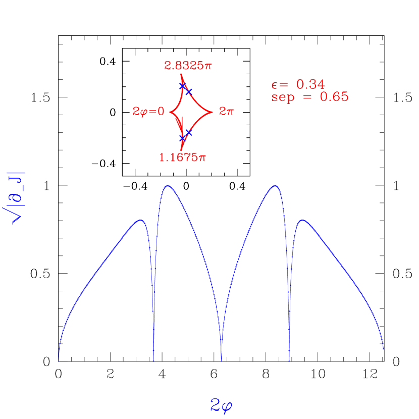
Figure 1: $\sqrt{|\partial_{-}J|}$ as a function of the phase angle of $\kappa=e^{i2\varphi}$: The central caustic has four cusps, and $|\partial_{-}J|$ has four zeros. Note that the total change of the phase angle along the caustic curve with four cusps is $4\pi$. (It is $2\pi$ for a triangular caustic curve and $8\pi$ for a hexagonal caustic curve. The total sum of the phase angle change along all the caustic loops of a binary lens is $8\pi$ which is a topological invariant related to the number of point masses that is two for a binary lens.)

The amplification coefficient $|\partial_{-}J|^{-1/2}$ increases toward a cusp ($\partial_{-}J=0$) where it diverges. Figure 1 shows the ”central caustic” of a binary lens with the fractional minor mass $\epsilon=\epsilon_{2}=0.34$ and the separation $\ell\equiv|x_{1}-x_{2}|=0.65$. The ”central caustic” (always across the lens axis, and here contains the center of mass inside) has four cusps, and $\sqrt{|\partial_{-}J|}$ has four zeros at $2\varphi=0,1.1675\pi,2\pi$, and $2.8325\pi$ where $2\varphi$ is the phase angle of  $\kappa=e^{i2\varphi}$ (in the Riemann sheet). The four blue crosses on the caustic curve mark the loci of the local maxima of $\sqrt{|\partial_{-}J|}$. Since the amplification of the “two extra images” is proportional to it, $|\partial_{-}J|^{-1/2}$ can be considered as the “strength” of the caustic curve. (As we will discuss later, the actual amplification of the two images also depends on the relative size of the source star with respect to the Einstein ring radius, which may be considered as a scale factor.) Note that the local minima of $|\partial_{-}J|^{-1/2}$ are very close to the off-axis cusps. We may loosely refer to it as that the cusps on the lens axis are stronger than the ones off the lens axis. In the same token, we can say that the cusp at $\varphi=0$ (near the dominant mass $\epsilon_{1}=0.66$) is stronger than the cusp at $\varphi=\pi$. In the case of MACHO-98-SMC-1, the second caustic crossing was closer to a cusp on the lens axis ($2\varphi=0$) than the first caustic to its nearest cusp ($2\varphi=2\pi$), and the caustic crossing amplification peak for the second caustic crossing is bigger than the first (see figure 1 and 2 in Rhie et al 1999). This lens ($\epsilon=0.34$ and $\ell=0.65$) also has two triangular caustic curves off the lens axis (and reflection symmetric with respect to the lens axis – real line here), and each has “topological charge” $1/2$. The eigenvectors $E_{\pm}$ rotate by $\pi$ around each triangular caustic curve (or “trioid”). The eigenvectors rotate by $2\pi$ around the central caustic “quadroid” in figure 1 which has “topological charge” $1$. These off-axis caustics are “weaker” than the caustics which cross the lens axis. For example, the maximum of $\sqrt{|\partial_{-}J|}$ on these “trioids” (closed curve that is smooth except at three cusps) $\approx 6.93$ which is about 7 times larger than the maximum on the “central caustic” (“quadroid”: closed curve that is smooth except at four cusps).

If $\partial_{-}J=0$, equations (10) or (13) becomes linear in $dz_{-}$, and one obtains a linear solution whose amplification depends linearly on the inverse of the distance of the source to the caustic:  $A_{\rm cusp}\propto 1/\delta$. When the source exits the caustic through a cusp, this image crosses the critical curve. This is the third image that diverges at a cusp crossing. The other two image solutions can be obtained by including the third order terms in the expansion of $\delta\omega_{2-}$ in (10). If the source is sufficiently small compared to the caustic curve, the probability of crossing the caustic through a cusp is small. Out of about ten caustic crossing binary lensing events discovered so far Alcock et al (1999), MACHO-97-BLG-28 was the only event where the crossing was through a cusp Albrow et al. (1999). The source star of the event MACHO-97-BLG-28 was a giant star. Most of the lensed stars in microlensing experiments are main sequence stars. Here, we consider caustic crossings away from cusps only.

If the source is sufficiently small, the curvature of the caustic curve can also be ignored, and we can assume that the luminosity variation of the light curve over the caustic crossing is largely determined by the critical behavior of the lensing amplification and the luminosity profile of the source star. If we let the line caustic be along the $y$-direction, the lensing amplification is independent of $y$, and we only need to know the “1-d luminosity profile” of the source in the normal direction, say $x$-direction, which is obtained by integrating the 2-d profile along the $y$-direction. It is worth emphasizing that the luminosity profile we probe directly in a line-caustic crossing microlensing event is the 1-d luminosity profile of the source star. (The “irregularities” of the stars such as star spots are not addressed here. The 1-d luminosity profile will depend on the position of the spots with respect to the direction of the caustic line.)

If the size of the star is $r_{\ast}$ (in units of Einstein ring radius), the luminosity profile in equation (2) can be rewritten in terms of the radial coordinate $r$ of the stellar disk using $h^{2}=1-r^{2}/r_{\ast}^{2}$.̃  We let $r^{2}=r_{\ast}^{2}~{}(x^{2}+y^{2})$ such that  $x$ and $y$ are the Cartesian coordinates of the unit stellar disk, and define a dimensionless 1-d luminosity function  $f(x)=\sum_{n}c_{n}f_{n}(x)$ based on the radial luminosity profile in equation (2).

$$f_{n}(x)\ \equiv\ \int h^{n}dy=\int_{0}^{\sqrt{1-x^{2}}}\left(1-r^{2}/r_{\ast}^{2}\right)^{n\over 2}dy=2b_{n}\left(1-x^{2}\right)^{n+1\over 2}\ ,$$ (23)

where $b_{0}=1,\ b_{0.5}=0.87362649,\ b_{1}=\pi/4$,  and $b_{2}=2/3$.

$$b_{n}\equiv\int_{0}^{1}\left(1-t^{2}\right)^{n\over 2}dt$$

The integrated flux is given by a byproduct of ${b_{n}}^{\prime}s$.

$$F_{n}\ \equiv\ \int h^{n}~{}dxdy=\int f_{n}~{}dx=4b_{n}b_{n+1}$$ (24)

We find $b_{1.5}=0.71849148$  and  $b_{3}=3\pi/16$, and

$$F_{0}=\pi~{};\quad F_{0.5}=2.51077224\approx{4\pi\over 5}~{};\quad F_{1}={2\pi\over 3}~{};\quad F_{2}={\pi\over 2}$$

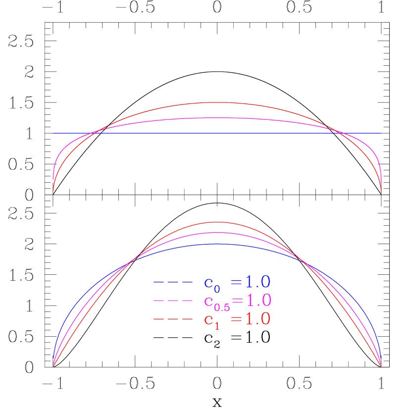
Figure 2: The luminosity profile functions across the diameter of the stellar disk (upper panel) and 1-d luminosity profile functions (lower panel) for $n=0,0.5,1,2$: The total flux emitted perpendicular to the disk (or toward an observer) has been normalized to $\pi$. In a line caustic crossing microlensing, one can effectively scan the 1-d luminosity profile in time.

Figure 2 shows normalized radial luminosity profile  $h_{n}\pi/F_{n}$ and 1-d luminosity profile $f_{n}\pi/F_{n}$. We have chosen the total flux to be $\pi$ for easy recognition of the peak values of the radial luminosity profile in the plot:   the peak values are $1,~{}\approx 5/4,~{}3/2$, and $2$ for $n=0,0.5,1$, and $2$ respectively. For the 1-d luminosity profiles, the peak values are given by $\pi/2b_{n+1}$:  $2.00,~{}2.19,~{}2.36$, and  $2.67$. Because of the integration in $y$, the limb-darkening effect is more accentuated in the 1-d luminosity profile compared to the radial luminosity profile of the stellar disk.

The amplification profile of the two extra images at a caustic crossing can be calculated using the luminosity profile $f(x)$ and the analytic form of the point source amplification function $A_{\pm}$ in equation (18).

$${\int fA~{}dx\over\int f~{}dx}\ \equiv G\quad;\qquad A\equiv A_{+}+A_{-}$$ (25)

Since the point source amplification function $A$ vanishes in one side of the caustic line, we may specify the segment of the one dimensional star (as defined by the 1-d luminosity function) that is inside the caustic, say, as given by an interval $[r_{\ast}a,~{}r_{\ast}]$  where $(a<1)$. Then, $A$ may be written as a function of $x$ accordingly.

$$A={1\over\sqrt{|\partial_{-}J|}}{1\over\sqrt{r_{\ast}}}{1\over\sqrt{x-a}}\ \equiv\ A_{c}A_{\ast}A_{x}$$ (26)

The first factor $A_{c}$ is determined by where on the caustic curve the crossing occurs. Figure 1 shows $A_{c}^{-1}$ for the central caustic curve of a lens with $(\epsilon,~{}\ell)=(0.34,~{}0.65)$. In this case, in a line caustic crossing, $A_{c}\sim 1$-$10$. The other triangular caustics we mentioned above but not shown here are “weaker” and $A_{c}\sim 0.15$-$1$ for a line caustic crossing. The second factor $A_{\ast}$ depends on the size of the star.

$$r_{\ast}=D_{1}\alpha_{\ast}={R_{\ast}\ D_{1}\over D_{1}+D_{2}}={\alpha_{\ast}\over\alpha_{E}}\ ,$$ (27)

where $\alpha_{\ast}$ and $R_{\ast}$ are angular (apparent) and the physical sizes of the star respectively, and $\alpha_{E}=R_{E}/D_{1}$ is the angular size of the Einstein ring radius. Here, $\alpha_{E}=1/D_{1}$ because we set $R_{E}=1$. If $\alpha_{E}\sim 1$ mas, and $\alpha_{\ast}\sim 1$ - $10\mu$as, then $A_{\ast}\sim 30$ - $10$.

If $c_{n}=1$ for a given $n$, the amplification profile function $G$ is determined by one function $f_{n}$, and we may define $G_{n}\equiv G_{|c_{n}=1}$. Then, for an arbitrary luminosity profile, $G$ is written as a linear combination of $G_{n}$’s.

$$G(a)={\sum_{n}\tilde{c}_{n}~{}G_{n}(a)\over\sum_{n}\tilde{c}_{n}~{}}:\qquad\tilde{c}_{n}=c_{n}~{}F_{n}~{};\quad\sum_{n}c_{n}=1$$ (28)

The appearance of the “new” coefficients $\tilde{c}_{n}$ is due to that the directly measurable quantity in lensing is the amplification of the images where the normalization is the total flux while the coefficients $c_{n}$’s have been defined based on the luminosity profile where the more relevant unit quantity is the peak luminosity. Since we need to be able to compare the microlensing measurements with theoretical calculations as well as measurements from other methods, it should be useful to consider the linear coefficients $c_{n}$ of the analytic luminosity profile functions as the basic parameters and feel free to redefine linear coefficients based on them as the needs arise.

Since the amplification factors $A_{c}$ and $A_{\ast}$ contribute to the amplification of the two extra images as overall scale factors, we define $g_{n}(a)$ that depends only on $A_{x}(a)$ such that $G_{n}(a)=A_{c}A_{\ast}g_{n}(a)$. Then, $G(a)=A_{c}A_{\ast}g(a)$ where the shape function $g(a)$ is given as follows.

$$g(a)={\sum_{n}\tilde{c}_{n}~{}g_{n}(a)\over\sum_{n}\tilde{c}_{n}~{}}$$ (29)

In an observed lightcurve, the “time” $a$ in units of the (relative) stellar radius $r_{\ast}$ should be replaced by the actual time variable $t$. If the caustic crossing occurs at $t=t_{cc}$ (when the center of the star crosses the caustic line: $a=0$), $t_{\ast}$ is the stellar radius crossing time, and $\iota$ is the incident angle of the source trajectory (the small angle between $\pm E_{-}$ and the source trajectory),

$$a={(t-t_{cc})~{}\cos\iota\over t_{\ast}}\ .$$ (30)

So, the time axis of an observed lightcurve depends on the stretch factor

$${t_{\ast}\over\cos\iota}={\alpha_{\ast}\over\mu\cos\iota}={r_{\ast}R_{E}\over v_{\perp}\cos\iota}={R\ast\over v_{\perp}\cos\iota}~{}{D_{1}\over D_{1}+D_{2}}\ ,$$ (31)

where $\mu=|\vec{\mu}|$ is the relative proper motion of the lens with respect to the source star (as seen from the observer) and $v_{\perp}=|\vec{v}_{\perp}|$ is the relative transverse linear velocity of the lens.

If the caustic line is at $x=0$, and the center of the star is at $x=a<0$, then the amplification profile of the partial images ($a\geq-1$) is given as follows.

$$g_{n}(a)\equiv{\int f_{n}A_{x}~{}dx\over\int f_{n}~{}dx}={1\over 2b_{n+1}}\int_{a}^{1}{(1-x^{2})^{n+1\over 2}\over\sqrt{x-a}}~{}dx$$ (32)

For the two full extra images of the star when it is completely inside the caustic curve ($a<-1$), the integration range should be extended to $[-1,1]$. The functions $g_{n}(a)$  in figure 3 and 4 show some of the characteristic effects of the luminosity profiles at a line caustic crossing:

1. The lightcurve becomes practically insensitive to the luminosity profile when the star is about two stellar radii away from the caustic line ($a=-2$).

2. In the immediate neighborhood of $a=-1$, the lightcurve rises rapidly and the curvature of the light curve changes from concave upward to convex. Thus, given a well-sampled lightcurve, the caustic entry “time” $a=-1$, where the limb of the star touches the caustic line producing two images joined at a critical point, can be read off from the lightcurve with a relatively small error. Past $a=-1$, the images become partial, and the loss of the flux due to the partial imaging causes the slope of the lightcurve to decrease leading to peak turn-over and rapid decline of the lightcurve.

3. The peaks are relatively broad, and the practically universal intersection points of the falling curves at $a=a_{f}\approx 0.28$ offer a natural distinction between the peak ($a<a_{f}$) and the tail ($a_{f}<a<1$). With increasing $n$  (the surface luminosity is more concentrated toward the center of the star with larger $n$), the rising curve of the peak becomes less steeper and the falling curve becomes more steeper. (The slope of $g_{\circ}$ diverges at $a=-1$.)

4. The peak crossing time where the lightcurve has the maximum amplification and the peak amplification value are sensitive to the luminosity profile. The peak crossing times are $a=-0.656,~{}-0.565,~{}-0.503$, and $-0.423$ for $n=0,~{}0.5,~{}1$ and $2$ respectively. (The peak crossing time of a point source is $a=0$.) The varying peak crossing times look a bit more impressive in unnormalized lightcurves Rhie (1999).

5. The tails ($a_{f}<a<1$) are dominated by the “linear behavior” except very near the end point ($a=1$). Thus, given a well-sample lightcurve, the caustic exit “time” $a=1$, where the limb of the star completely exits the caustic and the two extra images disappear, can be more or less read off from the lightcurve. The slope of the lightcurve can change abruptly ($n=0$) or smoothly ($n=0.5,1,2$)) at the end-point (see below). Near the end-point, the observed lightcurve is dominated by three normal images whose magnification behavior outside the caustic curve crucially depends on the proximity to a nearby cusp. (A cusp dominates the magnification behavior of the source plane around it more like the point caustic of a single and may be considered as a point caustic with directionality.) If the flux of the normal images is about 10% of the peak flux, the shape function may not be representative of the behavior of the observed lightcurve when $a\hbox{ \hbox to0.0pt{\raise 1.82986pt\hbox{$>$}\hss}\lower 2.79857pt\hbox{$\sim$} }0.8$. In the case of MACHO-98-SMC-1, the flux of the normal images was about $7\%$ of the peak flux for the second caustic crossing and about $10\%$ for the first caustic crossing Rhie et al. (1999). In the event MACHO-97-BLG-41, it was about $16\%$ for the central caustic crossing and about $30\%$ for the planetary caustic crossing Bennett et al (1999); Albrow et al. (1999).

6. The caustic crossing time, $a=0$, marks a most featureless part of the lightcurve.

In order to examine the the end-point behavior of the shape function $g_{n}(a)$, we rewrite the expression in (32) with $\xi=1-x$.

$$g_{n}(a)={1\over 2b_{n+1}}\int_{0}^{1-a}{(2\xi-\xi^{2})^{n+1\over 2}\over\sqrt{1-a-\xi}}~{}d\xi$$ (33)

For $a\approx 1$, the higher order term $\xi^{2}$ in the numerator can be ignored, and $g_{n}(a)$ scales in $(1-a)$ as follows.

$$g_{n}(a)\ \propto\ (1-a)^{n+2\over 2}$$ (34)

where the proportional constant is given as follows.

$${1\over 2b_{n+1}}\int_{0}^{1}{(2\eta)^{n+1\over 2}\over\sqrt{1-\eta}}~{}d\eta$$ (35)

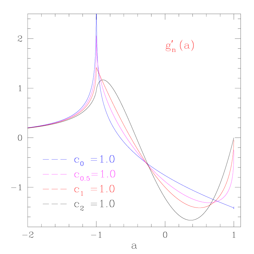
Figure 4: The derivatives $g_{n}^{\prime}(a)$:  at $a=-1$, the slope of the shape functions $g_{n}(a)$ change singularly. At the end-point ($a=1$), the slope is discontinuous for $n=0$, and continuous for the others.

Therefore, the derivative of $g_{n}$ vanishes at $a=1$ unless $n=0$, which can also be seen in figure 4. For a homogeneous model, the shape function $g_{\circ}$ has a finite slope at the end-point:   $g_{\circ}^{\prime}(1)=-\sqrt{2}$. This has an interesting ramification that every lightcurve of line caustic crossing should exhibit an abrupt change of the slope at the end-point. That is because the luminosity profile of any star has (or is believed to have) a sharp edge, or, equivalently, a nonvanishing $c_{\circ}$.

In order to gauge how well one can determine the luminosity profiles, we examine the linear models.

$$g_{Linear}(a)={\tilde{c}_{\circ}g_{\circ}(a)+\tilde{c}_{1}g_{1}(a)\over\tilde{c}_{\circ}+\tilde{c}_{1}}\ ;\qquad c_{\circ}+c_{1}=1$$ (36)

Figure 5 shows that the shape functions for $c_{1}=0.5$ and $c_{1}=0.6$ are almost indistinguishable in this plot. The intersection points are at $a=-0.76$ and $a=0.28$, and it will be necessary to sample the lightcurves in all three regions defined by the intersection points. The derivatives of the shape functions are shown in figure 6. The curvature changes at $a=-1$ marks the entry time, and it will be relatively easy to reconstruct the correct time in a fitting. The linear models with $c_{1}=0.5$ and $c_{1}=0.6$ show relatively constant slopes between $a=0.3$ and $0.8$ or so. The opposite trends of the slopes of $g_{\circ}$ and $g_{1}$ make the slope of the shape function of a typical main sequence star with a medium value of the linear limb-darkening parameter (say, $c_{1}=0.3-0.7$) more or less constant. This “linear behavior” of the lightcurve in the tail was measured for the first time in the event MACHO-98-SMC-1 Alfonso et al. (1998).

Figure 7 shows the differences $\delta g_{Linear}(a:c_{1})\equiv g_{Linear}(a:c_{1}+\delta c_{1})-g_{Linear}(a:c_{1}):\ \delta c_{1}=0.1$ for $c_{1}=0,0.1,....,0.9$. In this figure, the three regions divided by the intersection points are manifest. The larger the value of $c_{1}$, the higher the peak value at $a=-0.28$ and the larger amplitude of deviation. Thus, the smaller the value of $c_{1}$, the more demanding is the photometric accuracy and precision. In order to see the level of photometric accuracy we need, we normalize the difference curve $\delta g_{Linear}(a:c_{1})$ by $g_{Linear}(a:c_{1}+0.5\delta c_{1})+0.2$ as an example. Figure 8 shows the normalized difference curves. In order to determine the linear limb-darkening parameter $c_{1}$, one needs to be able to reconstruct the shape function, and this requires that all three regions defined by the intersections points $a=-0.76$ and $a=0.28$ be sampled fairly. The differences in tails look more discriminatory. However, the tails are more susceptible to the effects of the normal images and blending, and should be interpreted properly case by case. In an observed lightcurve, the determination of the scale factors $A_{c}$ and $A_{\ast}$ can be compromised if one overinterprets the “linear behavior” of the tails.

In summary, we have analyzed the magnification behavior of the two extra images that appear and disappear in a line caustic crossing binary microlensing. We have identified the shape function of the lightcurve of the two extra images and examined its dependence on the luminosity profile of the lensed star. We also discussed the multiplicative factors that determines the overall amplification and the ones that scale the time axis in an observed lightcurve. We suggest that it is important to sample the lightcurve fairly in all three regions that are defined by the intersection points. The span of the lightcurve that is affected by the luminosity profile is about $3r_{\ast}$  ($a=[-2,1]$). In the case of linear models, we estimate from figure 8 that the photometric accuracy of $0.3$-$0.8~{}\%$ is required to be able to determine the linear limb-darkening parameter $c_{1}$ with precision of $\delta c_{1}=0.1$. It is similar to the estimation made for the eclipsing binary method by Popper (1984). In lensing, the signal lies in magnification while it is in absorption in the case of eclipsing binaries. Thus, microlensing will have advantage for fainter stars.

Figure 3: Light curves of the two extra images of stars with luminosity profiles given by $f_{n}:n=0,0.5,1,2$. $a$ is the position of the center of the stellar disk with respect to the caustic line in units of the radius of the star $r_{a}st$. The caustic line touches the limb of the star from inside a caustic at $a=-1$ and leaves the caustic at $a=1$. The luminosity profiles are indistinguishable when the star inside the caustic line is about one diameter away from the caustic ($a=-2$). The peak crossing times are sensitive to the luminosity profiles. The peak crossing times are at $a=-0.656,~{}-0.565,~{}-0.503$, and $-0.423$ for $n=0,~{}0.5,~{}1$ and $2$.

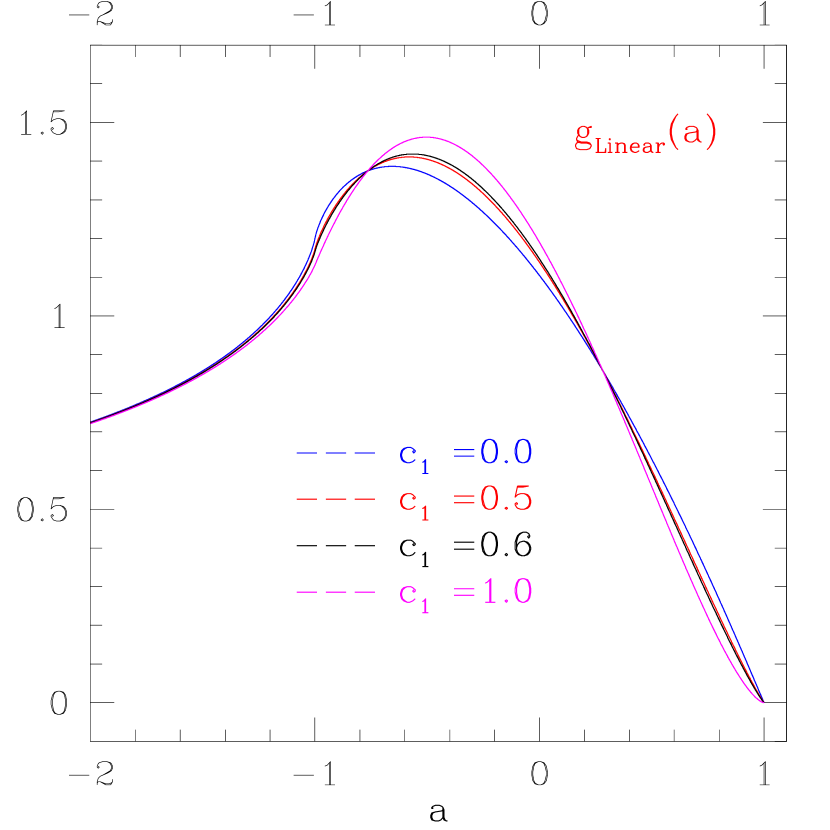
Figure 5: Light curves of the linear limb-darkening models: $g_{\circ}$ and $g_{1}$ determine the intersection points $a=-0.76$ and $0.28$, and the shape functions of linear models distributed in between $g_{\circ}$ and $g_{1}$. The typical linear limb-darkening parameters $c_{1}=0.5$ and $c_{1}=0.6$ are indistinguishable in this plot.

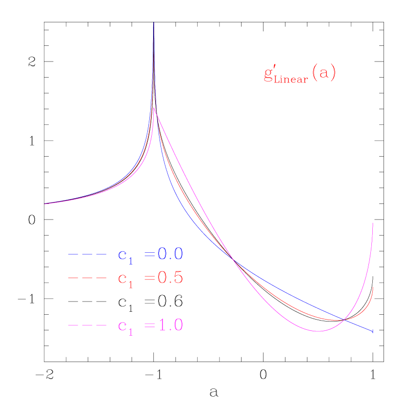
Figure 6: The linear models with $c_{1}=0.5$ and $0.6$ show relatively constant slopes between $a\approx 0.3$-$0.8$. Toward the end-point, the slopes change rapidly from $g^{\prime}\approx-1.2$ to $-\sqrt{2}c_{\circ}$.

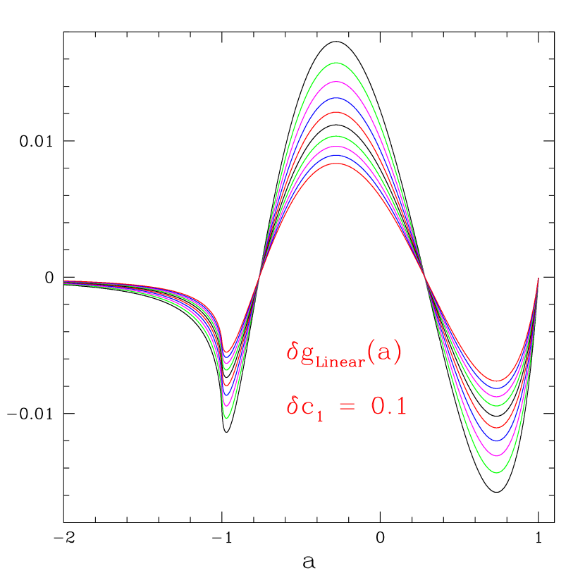
Figure 7: Difference lightcurves for linear models with $c_{1}$ values that differ by $\delta c_{1}=0.1$:  $\delta g_{Linear}(a:c_{1}+\delta c_{1})-\delta g_{Linear}(a:c_{1}):~{}\delta c_{1}=0.1$ for $c_{1}=0.0,...,0.9$. The difference lightcurve with the largest amplitude is for $c_{1}=0.9$.

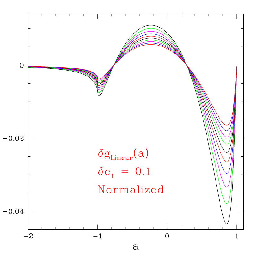
Figure 8: Normalized difference lightcurves for linear models with $c_{1}$ values that differ by $\delta c_{1}=0.1$:  the difference lightcurves in figure 7 have been divided by $g(a:c_{1}+0.5\delta c_{1})+0.2$. The baseline value $0.2$ we chose here as an example amounts to $\approx 12\%$ of the peak amplification. In order to determine the linear limb-darkening parameter $c_{1}$ with $\delta c_{1}=0.1$, photometric accuracy of $0.3$-$0.8~{}\%$ is needed.

References

- Abt (1993) Abt, H. 1993, Ann. Rev. Astron. and Astroph., 21, 343
- Alfonso et al. (1998) Alfonso, C., et al. 1998, A&A, 37, L17
- Alfonso et al. (2000) Alfonso, C., et al. 2000, ApJ, 532, in press (astro-ph/9907247)
- Albrow et al. (1999) Albrow, M. D., et al. 1999, ApJ, 512, 672
- Albrow et al. (1999) Albrow, M. D., et al. 1999, ApJ, 522, 1011
- Albrow et al. (1999) Albrow, M. D., et al. 1999, ApJ, Submitted (astro-ph/9910307)
- Alcock et al. (1999) Alcock, C., et al. 1999, ApJ, 518, 44
- Alcock et al (1999) Alcock, C., et al. (MACHO collaboration) 1999, ApJ, Submitted (astro-ph/9907269)
- Bennett et al (1999) Bennett, D., et al. (MPS collaboration) 1999, Nature, 402, 57 (astro-ph/9908038)
- Bennett & Rhie (1996) Bennett, D. P., and Rhie, S. H. 1996, ApJ, 472, 660
- Bourassa, Kanotowski, & Norton ( 1973) Bourassa, R. R., Kantowski, R., and Norton, T. D., 1973, ApJ, 185, 747
- Claret, Díaz-Cordovés, & Geménez ( 1995) Claret, A., Díaz-Cordovés, J. and Geménez, A. 1995, A&A, 114, 247
- Díaz-Cordovés & Giménez (1992) Díaz-Cordovés, J., and Giménez, A. 1992, A&A, 259, 227
- Díaz-Cordovés, Claret, & Geménez (1995) Díaz-Cordovés, J., Claret, A., and Geménez, A. 1995, A&A, 110, 329
- Gilliland & Dupree (1996) Gilliland, R. L., and Dupree, A. K. 1996, ApJ, 463, L29
- Gray (1995) Gray, D. F. 1995, ”The Observation and Analysis of Stellar Photosphere”, Cambridge University Press
- Kurucz (1991) Kurucz, R. L. 1991, Harvard Preprint 3348
- Milne (1921) Milne, E. A. 1921, MNRAS, 81, 361
- Popper (1984) Popper, D. M. 1984, AJ, 89, 132
- Rhie (1997) Rhie, S. H. 1997, ApJ, 484, 63
- Rhie & Bennett (1996) Rhie, S. H., and Bennett, D. P. 1996, Nucl.Phys.Proc.Suppl. 51B, 86-90
- Rhie & Bennett (1999) Rhie, S. H., and Bennett, D. P. 1999, astro-ph/9999000
- Rhie et al. (1999) Rhie, S., et al. (Microlensing Planet Search collaboration) 1999, ApJ, 522, 1037
- Rhie et al. (2000) Rhie, S., et al. (Microlensing Planet Search collaboration) 2000, ApJ, 532, in press (astro-ph/9905151)
- Rhie (1999) Rhie, S. H. 1999, “The Identification of Dark Matter”, World Scientific, ed., Spooner, N., and Kudryavtsev, V. (astro-ph/9903024)
- Schneider, Elhers, & Falco (1992) Schneider, P., Elhers, J., and Falco, E. E. 1992 “Gravitational Lenses”, Springer-Verlag
- Schneider & Wagoner (1987) Schneider, P., and Wagoner, R. V. 1987, ApJ, 314, 154