Caltech Faint Galaxy Redshift Survey X: A Redshift Survey in the Region of the Hubble Deep Field North

Abstract

A redshift survey has been carried out in the region of the Hubble Deep Field North using the Low Resolution Imaging Spectrograph at the Keck Observatory. The resulting redshift catalog, which contains 671 entries, is a compendium of our own data together with published LRIS/Keck data. It is more than 92% complete for objects, irrespective of morphology, to $R=24$ mag in the HDF itself and to $R=23$ mag in the Flanking Fields within a diameter of 8 arcmin centered on the HDF, an unusually high completion for a magnitude limited survey performed with a large telescope. A median redshift $z=1.0$ is reached at $R\sim 23.8$.

Strong peaks in the redshift distribution, which arise when a group or poor cluster of galaxies intersect the area surveyed, can be identified to $z\sim 1.2$ in this dataset. More than 68% of the galaxies are members of these redshift peaks. In a few cases, closely spaced peaks in $z$ can be resolved into separate groups of galaxies that can be distinguished in both velocity and location on the sky.

The radial separation of these peaks in the pencil-beam survey is consistent with a characteristic length scale for the their separation of $\approx$70 Mpc in our adopted cosmology ($h=0.6,\Omega_{M}=0.3$, $\Lambda=0$). Strong galaxy clustering is in evidence at all epochs back to $z\leq 1.1$.

A near-infrared selected sample with $K<20$ was also constructed in this field. Extremely red objects with $R-K>5.0$ comprise 7% of the total $K$-selected sample. This fraction rises rapidly towards fainter $K$ mag, reaching about 10% at $K\sim 19.7$.

We have attempted to identify the radio sources in the region of the HDF. The secure radio sources seem to divide into two classes. The first have reasonably bright galaxies at moderate redshifts as optical counterparts, while the second, comprising about 1/3 of the total, have extremely faint optical counterparts ($R\geq 25$ mag). These do not represent a continuous extrapolation in any property ($z$ or dust content) of the first group.

We identify $\sim$2/3 of the secure mid-IR sources in the region of the HDF with normal galaxies with $z<1.3$. The ratio of the mid-IR to optical flux increases as $z$ increases, but this is due primarily to selection effects, and the same trend is seen in the radio sources. We suggest that the mid-IR emission is more tightly coupled to the rate of ongoing star formation than is the radio emission.

We also demonstrate that the best photometric redshift techniques are capable of reaching a precision of $\sigma[(z_{phot}-z_{spec})/(1+z_{spec})]=0.05$ for the majority of galaxies with $z<1.3$.

The two broad lined AGNs with $z<3$ are the brightest objects in the redshift peak at $z\sim 0.96$.

May 24, 2000

On December 2, 1999, I archived in the LANL server a preprint (Astro-ph/9912048) of the paper “Caltech Faint Galaxy Redshift Survey X: A Redshift Survey in the Region of the Hubble Deep Field North” by Judith Cohen, David Hogg, Roger Blandford, Lennos Cowie, Esther Hu, Antoinette Songaila, Patrick Shopbell and Kevin Richberg. This paper is in press in the ApJ. The paper as submitted to Astro-ph at that time did not contain certain key figures and tables.

The text of this paper has today been replaced with a version which contains all the figures and tables, including the galaxy redshifts.

Unfortunately, I and my group, being small (because I have received no federal funding for this research for several years) have not finished two final pieces of analysis: (1) a paper on the evolution in the galaxy luminosity function and (2) a paper on the relationships between broadband colors, morphologies, and narrow spectral features (lines and breaks). I therefore request that the redshifts not be used for projects which are substantially similar to either of these two projects until I have submitted such papers to astro-ph. I expect this to happen by 2000 October. Thank you very much.

Judy Cohen

1 Introduction

The Hubble Deep Field North (henceforth HDF) is a region of intense astrophysical interest. The selection of the field and the HST campaign in the HDF are described by Williams et al. (1996). The field was chosen to be a “typical” high galactic latitude field with no known bright sources in the x-ray, UV, optical, IR and radio passbands, and no known nearby ($z<0.3$) galaxy clusters. The superb multi-color WFPC2 images taken by the Hubble Space Telescope reach to $B\sim 29$ and with their 0.1 arcsec spatial resolution provide an unprecedented view of the distant Universe.

There has been follow up of these beautiful HST images of the HDF in most wavelength ranges. These include the deep radio survey of Richards et al. (1998) with the VLA, which extends into the Flanking Fields around the HDF, and the survey by Hughes et al. (1998) in the sub-mm. Space-based IR followup with NICMOS was done by Thompson, Storrie-Lombardi & Weymann (1999) and by Dickinson (1999), while Aussel et al. (1999) report on a survey of the HDF with ISO. From the ground, Hogg et al. (1997) imaged two subregions to $K=25.2$ at 2.2 $\mu$.

The strong interest in this field has also led to major efforts by several groups to obtain redshifts for the galaxies in this field to study star formation, galaxy evolution and galaxy clustering, as well as to aid in the interpretation of data at other wavelength regimes where redshifts are more difficult/impossible to determine. Given the magnitude limit for practical redshift determinations, extensions beyond that regime using photometric redshifts have been actively pursued by various groups and applied to the HDF to explore star formation rate at very high $z$, e.g. Connolly et al. (1997).

We provide here a compilation of our own work over the past few years towards a redshift survey in the HDF and its environs with published work to produce a very complete magnitude limited redshift survey of objects in this region. All spectra, both our own and from the literature, were taken with the Low Resolution Imaging Spectrograph (henceforth LRIS) (Oke et al. 1995) at the Keck Observatory, without which this effort would be impossible.

We present the redshift catalog in §2, which greatly extends our earlier work in the region of the HDF (Cohen et al. 1996, henceforth C96) from 140 objects to 671 objects with redshifts. After a brief discussion of the extremely red objects in §2.9, we comment on the accuracy of photometric redshift techniques in §3. We then proceed in §4 to discuss the distribution in redshift of the sample, the nature of the strong redshift peaks and large scale structure. A sketch of the luminosity and density evolution of galaxies in the region of the HDF is given in §5. We follow with a discussion of the HDF as seen in other wavelength regimes (radio, mid-IR and sub-mm) in §6, and then summarize our results in §7.

We adopt the cosmological parameters $H_{0}=60$ km s^-1 Mpc^-1 and $\Omega_{M}=0.3$ with $\Lambda=0$, as in earlier papers in this series.

2 The Redshift Catalog

2.1 Observing Procedure

The goal established by the Caltech group was to carry out a magnitude limited survey of objects in the region of the HDF to a limit of $R=24$ for the HDF itself and to a limit of $R=23$ mag for the region within a field with a diameter of 8 arcmin centered on the HDF, but excluding the HDF itself, which we call the Flanking Fields. The size of the region we included in the spectroscopic survey was determined by the length of the LRIS slit in the multislit mode. Hogg et al. (1999) (henceforth H99) present a four-color photometric catalog for the region of the HDF covering this area; their $R$ catalog is adopted here to define the magnitude limited samples. Objects were included in the sample independently of their morphology although, of course, there may be extremely extended, low surface brightness sources that would not be detected.

Cowie, Hu & Songaila (1995) in general pursued more targeted projects, and include the majority of their spectra in the region of the HDF in the present compilation.

Observations were carried out and analyzed in a manner similar to that described in Cohen et al. (1999b) from 1996 to 1999 using many slit masks in the region of the HDF. The gratings used and the resulting spectral resolution and spectral coverage are not uniform throughout the catalog, although most of the spectra were obtained with the 300 g/mm grating, giving a spectral resolution with a 1 arcsec slit of 10 Å. Spectra of some of the fainter objects were obtained with a 155 g/mm grating which became available in 1998; the sky subtraction is more difficult at lower dispersion and most of the objects with dubious features redward of 6000 Å were subsequently re-observed with a higher dispersion grating. A few objects were observed with the higher dispersion 600 g/mm gratings. A typical uncertainty in redshift is 200 km s^-1 in the observed frame for an object with a spectrum taken using the 300 g/mm grating and with $R<23$.

2.2 Sources of Published Data

The sources of published data at lower redshifts ($z\lesssim 1.3$) are Phillips et al. (1997) (from the Lick Deep Group) and the work of the Caltech and of the Hawaii group published in C96. At high redshift ($z>2)$, the results of Steidel (Steidel et al. 1996, Dickinson 1998, Steidel et al. 1999) and of the Lick Deep Group (Lowenthal et al. 1997) are combined with single very high redshift galaxies found by Spinrad et al. (1998), Weymann et al. (1998) and Waddington et al. (1999). Five unpublished redshifts from C. Steidel (private communication) are also included.

As the catalog was compiled, any discrepancies between multiple observations of the same object were reconciled. In most cases with duplicate observations, the agreement was superb ($\Delta(z)\leq 0.005$). For about 20 galaxies with more than one spectrum, the initial redshifts were wildly discrepant, but these cases were resolved by one person (JGC and sometimes also LLC) looking at all the available spectra of the galaxy. Details for the small number of galaxies for which the final redshift adopted in this catalog is different from the previously published value can be found in the Appendix.

Table 1 lists the sources of the data and the number of objects included from each.

2.3 Matching the Photometric and Redshift Catalogs

The coordinate system in the HDF itself, defined now by VLA observations, has changed very slightly with time as described in Williams et al. (1996), while the definition of the coordinate system in the Flanking Fields is described in H99. As will be shown in §6.1, the coordinate system we use agrees with that defined by the VLA to within 0.1 arcsec in RA and also in Dec. The redshift catalog was constructed beginning with coordinates defined by the observer for each object. Then the small systematic offsets in RA and Dec between each set of redshift data were determined, and the appropriate (small) corrections were made to the object coordinates.

The matching of the redshift catalog onto the photometric catalog of H99 was non-trivial, particularly in the HDF, where the depth of the sample increases the crowding, and particularly for objects with $R>23$. The matching was done automatically for objects with $R<23.5$ mag; if only one object in the photometric catalog was within 1.5 arcsec of the position of an object in the redshift catalog, it was accepted as the match.

Objects fainter than $R=23.5$ as well as brighter ones with multiple or no matches in the photometric catalog of H99 were examined individually. In most cases, the match was obvious. In all but a few of the remaining cases, the nature of the problem became apparent after checking for close pairs, coordinate errors, bookkeeping errors, etc. There are a very small number of objects with uncertain matches, and these are noted in the redshift catalog.

There are some objects in the region of the HDF for which redshifts have been obtained which are genuinely too faint for the photometric catalog of H99. These have been included as a supplemental table in the photometric catalog (see H99 for details). They are indicated by notes in Table 2.

2.4 Close Pairs

The SExtractor algorithm (Bertin & Arnouts 1996) with the parameters adopted by H99 in some cases fails to separate close pairs with separations of under 1.5 arcsec. When there are two entries in the redshift table, but a single corresponding entry in the photometric catalog, photometry of the two components can be found in a supplemental table in H99 and there is an appropriate note in Table 2. For purposes of computing completeness, we assume that the single entry representing the pair in the primary photometric table has been matched only if both members of the pair have redshifts.

A discussion of the objects that are genuine close pairs rather than projections and the implications for merger rates is given in Carlberg et al. (2000).

2.5 Completeness

In the HDF itself only a few faint objects near the magnitude cutoff are missing from the catalog. In the Flanking Fields, however, some brighter objects were missed initially due to problems in defining the sample. Since the final photometric catalog only became available very late in the project, it was not possible to pick up all the missing objects in the limited telescope time available. Hence some of the missing objects in the Flanking Fields are not near the faint limit, and spectroscopic observations, had they been carried out, would undoubtedly have yielded a definite redshift.

The redshift completeness fraction is very high, as is shown in Figure 1a,b, which also shows the cumulative redshift completeness for objects brighter than a given $R$ mag. Of the 114 objects with $R<24$ in the $R$ band photometric catalog of H99 in the HDF, only 8, the brightest of which has $R=23.2$, are missing from the redshift catalog. The completeness is thus 93%. In the Flanking Fields within an area with a diameter of 8 arcmin centered on the HDF, and excluding the HDF itself, there are 434 objects in the $R<23$ photometric sample, and the redshift completeness there also exceeds 92%.

The eight objects in the HDF in the $R$-selected sample ($R<24$) that do not have spectroscopic redshifts at the present time and hence that are not included in Table 2b are listed in an appendix. Many of these have been observed more than once. It should be empahsized that the objects in the region of the HDF that were observed, but for which redshifts have not been determined yet, are not included in the tables nor considered when calculating completeness.

2.6 Galaxy Spectral Classes and Redshift Quality Classes

The galaxy spectral classification scheme adopted here is that of Cohen et al. (1999b). To review briefly, “${\cal E}$” galaxies have spectra dominated by emission lines, “${\cal A}$” galaxies have spectra dominated by absorption lines, while “${\cal I}$” galaxies are of intermediate type. Galaxies with broad emission lines are denoted as spectral class “${\cal Q}$”. Starburst galaxies showing the higher Balmer lines (H$\gamma$. H$\delta$, etc.) in emission are denoted by “${\cal B}$”, but for such faint objects, it was not always possible to distinguish them from “${\cal E}$” galaxies.

All the spectral classifications were done by JGC.

The spectral classifications are most accurate for the brighter galaxies with $z<1.2$. For the fainter ones, emission lines are easier to detect than absorption lines, and the distinction between galaxy spectral classes “${\cal E}$”, “${\cal EI}$” and “${\cal I}$”, which depends critically on the presence or absence of the Balmer lines in absorption near 4000Å in the rest frame, becomes blurred. In addition, for some galaxies with low redshifts, the spectral region covered did not extend sufficiently to the blue, and the 4000 Å region was lost, so the distinction between “${\cal E}$”, “${\cal EI}$” and “${\cal I}$” could not be made with the material available. Notes to the table indicate such concerns.

Spectral classes for galaxies with $z>1$ were not assigned in a completely consistent manner. A galaxy whose spectrum showed emission at 3727 Å and absorption at the 2800 Å Mg doublet, a fairly typical combination at $z\sim 1.2$, could be assigned to spectral class “${\cal E}$”, “${\cal EI}$” or “${\cal EA}$”.

The spectra of galaxies with $z>2$ could not be classified as carefully. Most of these are from published data, and in some cases the original spectra were not available to JGC. In such cases (and also for lower $z$ objects where the spectra were not available to JGC), the spectral class is given as “${\cal X}$”. (Unless otherwise noted, when a spectral type is required, for example to define the symbol in a figure, these are assumed to be “${\cal E}$” galaxies.)

Redshift quality classes were assigned following Cohen et al. (1999b). One additional class was added here for extremely faint objects ($R>24.3$) observed by the Caltech group which turned up serendipitously in slitlets intended for some brighter nearby galaxy and which show only a single emission line with no sign of a continuum. In our previous work, for spectra showing only a single emission line, the assumption was always made that this line is the [OII] line at 3727 Å. However, in these particular cases, the objects are so faint that we have instead assumed that the emission line is Ly$\alpha$. There are seven galaxies in this category assigned to redshift quality class 11. These are probably similar to the $z\sim 4$ single emission line galaxies found by Hu, Cowie & McMahon (1998). There is one additional galaxy which would have been in this category except that a second spectrum is available from Lowenthal et al. (1997) which confirms the $z\sim 3$ redshift.

No redshift quality class is assigned for the “${\cal X}$” galaxies.

2.7 The Merged Redshift Survey

Table 2a,b contains the merged redshift table. The objects are in order of RA, with those in the the Flanking Fields in Table 2a, and those in the HDF itself in Table 2b. The coordinates listed are those of H99, from the matching of the redshift observations to the $R$-band object catalog. The $R$ magnitude is that of the matched object from H99 as well. Then follows the redshift, the redshift quality class, the galaxy spectral class and the source(s) for the redshift determination.

Following the main catalog, Table 3 contains similar data for 15 objects just outside the survey boundary (a diameter of 8 arcmin from the center of the HDF).

There are 671 entries. Of these, 146 are within the three WF chips of the HDF itself, 510 are in the Flanking Fields within a diameter of 8 arcmin centered on the HDF, but outside the HDF itself, and 15 are just outside the spatial boundary of the survey. There are 11 spectroscopically confirmed galactic stars in the HDF and 42 spectroscopically confirmed stars in the Flanking Fields.

Figure 2 displays the HST image of the HDF from Williams et al. (1996) with the objects and their redshifts marked. Figure 3 is a similar overlay of four panels identifying the objects in the redshift survey on each of the four quadrants of the the HST composite image of the Flanking Fields. A color coding of the galaxy spectral class is used for objects with $z<1.0$.

2.8 Median Redshift

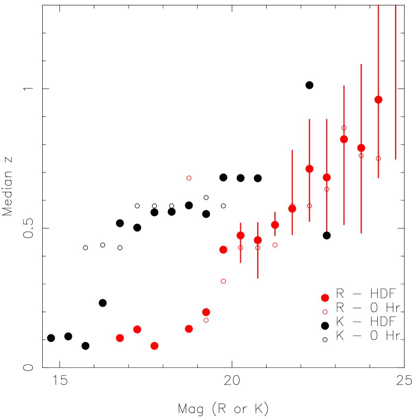
Figure 4: The median redshift is shown as a function of the $R$ and of the $K$ mag for the sample in the region of the HDF and for the sample in the field J0053+1234 from Cohen et al. (1999a). The first and last quartiles for the HDF sample are indicated for $R$ by error bars only when there are more than 10 galaxies in a bin.

The median redshift as a function of $R$ and of $K$ is shown in Figure 4 and given in Table 4. The first and last quartiles are also tabulated for $R$. Although redshifts have been determined for more than 92% of the sample to its defined magnitude limits, at the fainter magnitudes these are biased by the incompleteness of our spectroscopic survey, in particular, by the detection efficiency, or lack thereof, in the regime $1.4<z<2.0$.

We have corrected the sample in an approximate manner by adding in a rough representation of the set of missing galaxies in the interval $1.4<z<2.0$ derived from the magnitude distribution of the sample near $z\sim 1$. Specifically for the missing galaxies, we assumed the luminosity function to be the same as that in the interval $1.0<z<1.2$ and the comoving density to be constant with $z$ in this regime. The augmented set of galaxies then has a redshift distribution whose medians and quartiles are listed in table 4 as “corrected” values.

Our redshift catalog for the region of the HDF becomes highly incomplete at $R>24$, and it is unclear how many low $z$ objects should be added at that magnitude level that were rejected by the UV-dropout selection technique used to select samples for spectroscopy by various groups.

Table 4 shows that a median $z$ of 1.0 is reached at $R=24.2$ among the observed sample in the region of the HDF. This is reduced to $R=23.8$ when one corrects as described above for the galaxies in the regime $1.4<z<2.0$ whose redshifts were probably not determined in our survey.

2.9 Extremely Red Objects

We adopt the criterion that objects with $R-K>5.0$ are considered extremely red objects (EROs). The $K-$selected sample from H99 in the region of the HDF is complete for $K\lesssim 19.8$ and, as is shown in Figure 4 of H99, covers an area only slightly larger than that of the spectroscopic sample. There are 33 EROs out of 487 objects in the photometric catalog, which is 7% of the total $K-$selected sample, or 8% of the total sample excluding galactic stars. The fraction of EROs as a function of $K$ rises rapidly from 4% of the objects at $K\sim 18.3$ to 10% at $K\sim 19.7$. The reddest ERO has $R-K=6.0$. Only one of these EROs in the region of the HDF, H36443_1133, has a redshift. Its spectral class is, as expected, “${\cal A}$” with $z=1.05$.

There is an additional ERO in this sample with a redshift, F37016_1146, with $z=0.884$, which is a radio source and is fainter than the limit of the H99 photometric survey in $R$. This galaxy shows 3727Å in emission and is discussed in Barger, Cowie & Richards (2000).

The nature of the ERO population is still uncertain. Some, particularly the most luminous and reddest ones, may be distant dusty mergers or starbursts, but we proposed in Cohen et al. (1999a) that the majority of the EROs in this color and magnitude range are old galaxies at $z\sim 1.5$. Although EROs are very rare in optically selected samples, their presence in substantial numbers in faint infrared selected samples such as the study of NICMOS images by Benitez et al. (1999), as well as our work and that of others, is by now well established, in contrast to the claims of Kauffmann & Charlot (1998). Their existence forces a reconsideration of models for the formation of elliptical galaxies in which the bulk of such galaxies form at $z\sim 1$ (e.g. that of Kauffmann, Charlot & White 1996).

3 A Blind Check of Photometric Redshifts

We have utilized our new merged catalog of redshifts for objects in the HDF from Table 2b to carry out a second blind test of photometric redshifts in a spirit similar to our first test, Hogg et al. (1998). The advantage of the present test is that the set of spectroscopic redshifts known to us but not available to the developers of photometric redshift algorithms is significantly larger than it was at the time of our first test. In addition, the redshifts used in Hogg et al. (1998) were preliminary values, while those of Table 2 are final redshifts.

Three photometric redshift schemes were chosen to span the range of techniques used. Wang, Bahcall & Turner (1998) use polynomial fits to colors, while Sawicki, Lin & Yee (1997) and Lanzetta, Yahil & Fernandez-Soto (1996) use template spectra of galaxies. The catalogs of predicted photometric redshifts were taken from each group’s WWW site as listed in their papers.

In each case, the list of redshifts for the training set of galaxies was checked against the entries in Table 2b. If they agreed to within the larger of 5% or 0.05, the object was considered a good calibrator. If they disagreed (often because the preliminary redshift adopted by Hogg et al. 1998 was subsequently substantially modified) the object was considered as an unknown. To this we add the galaxies in the HDF whose redshifts, even in preliminary form, were not available for each of the photometric redshift training sets. This is a number which varies depending on when the photometric redshift technique was developed and applied to the HDF, as more calibrating galaxies with spectroscopic redshifts became available with time.

We compute the mean and dispersion of the difference between the predicted redshifts from the photometric technique and the measured spectroscopic redshift for this set of unknowns for each of the three groups, as well as the correlation coefficient. These are calculated in units of (1+z) to avoid errors in small redshifts artificially inflating the results. In each case, H36396_1230 (a probable AGN) was omitted; none of the groups came close to predicting this object’s redshift.

Figure 5 illustrates the results for the three techniques in the low $z$ regime ($z<1.5$). A distinction is made between spectroscopic redshifts that are secure and those that are more uncertain (i.e. have quality class 3, 8 or 9). There are a few outliers, some of which are beyond the range displayed, but most of the galaxies show a small dispersion in $(1+z)$ between the predicted redshift and the measured spectroscopic value.

Table 5 gives the results for each of the three groups, tabulated separately for $z<1.5$ and for $z>1.9$. The first column contains the total number of galaxies with new spectroscopic redshifts, followed by the mean and 1$\sigma$ dispersion of $\Delta(1+z)$. This is repeated after eliminating the outliers at more than 4$\sigma$.

At low $z$, once the outliers comprising ${\sim}10$% of the objects are eliminated, both the astrophysically motivated scheme of Sawicki et al. (1997) and the polynomial fitting of Wang, Bahcall & Turner (1998) give remarkably good results. At the time that Lanzetta et al. (1996) carried out their work, fewer spectroscopic redshifts were available to use as calibrators, which may explain the somewhat larger dispersion between their photometric redshifts and the recent spectroscopic measurements.

At high $z$, the astrophysically motivated schemes work somewhat better than the polynomial fitting, but all perform surprisingly well.

There are four galaxies that are rejected as outliers by all of the photometric redshift techniques tested here. Three of these galaxies have uncertain redshifts and one of the three is 1.7 arcsec away from a much brighter galaxy, which may affect its photometry. The fourth outlier has a secure redshift. However, the fraction of outliers is small, the success rate is very high, and the precision of the predictions is extremely good.

This, our second blind test, has again demonstrated that photometric redshifts with suitable algorithms are capable of producing highly accurate predictions for galaxy redshifts over the magnitude and redshift intervals for which they have been calibrated. The best of the three schemes tested predicts (1+z) to less than 5% for more than 90% of a realistic sample of galaxies over the full range of $z$ for which training galaxies exist. A dispersion of only 15%, still remarkably small, covers the maximum found among the three schemes.

The current lack of training sets of galaxies with spectroscopically determined redshifts in the regime $1.2<z<2.0$ is a problem which should be resolved shortly through the efforts of several groups, including our own. Photometric redshift techniques are becoming useful tools for many problems, including determining luminosity functions and star formation rates, choosing samples for spectroscopy, and related issues. It is of course a requirement that suitable multi-color high precision photometry exist and that the spatial resolution available is sufficient to avoid image overlapping within the magnitude regime of interest.

4 The Distribution in Redshift

4.1 The Strong Redshift Peaks

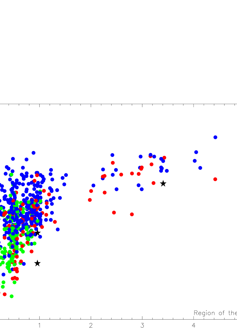
Figure 6: The $R$ mag is shown as a function of redshift for galaxies in the region of the HDF. Blue circles denote “${\cal E}$” galaxies, green circles denote “${\cal I}$” galaxies, while red circles denote absorption line “${\cal A}$” galaxies. QSOs/broad lined AGNs are indicated by black stars.

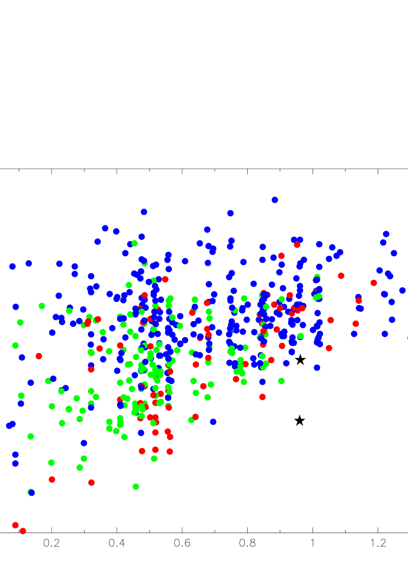
Figure 7: The $R$ mag is shown as a function of redshift for galaxies in the region of the HDF for $z<1.6$. The symbols are the same as those of Figure 6.

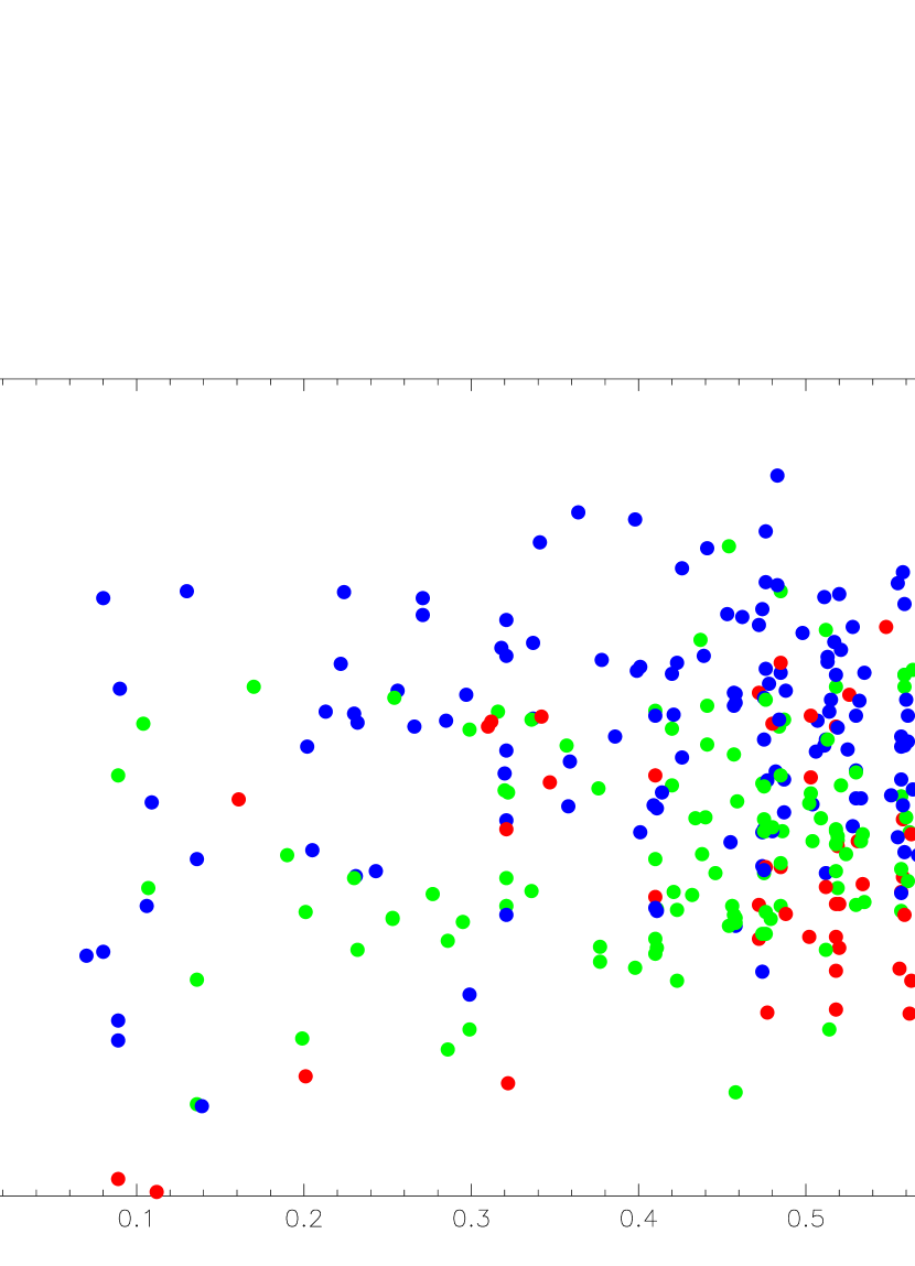
Figure 8: a) The $R$ mag is shown as a function of redshift for galaxies in the region of the HDF for $z<0.7$ (figure 8a) and for $0.6<z<1.4$ (figure 8b). The symbols are the same as those of Figure 6.

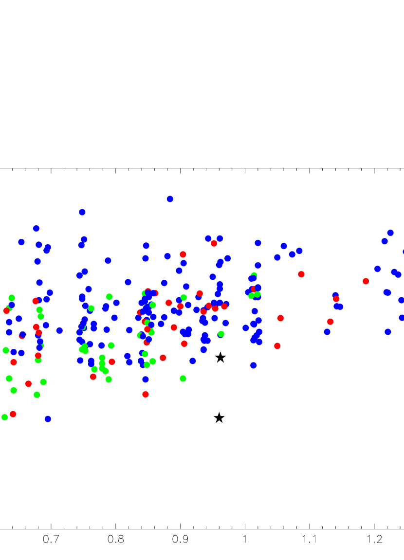
Figure 8: b) The $R$ mag is shown as a function of redshift for galaxies in the region of the HDF for $z<0.7$ (figure 8a) and for $0.6<z<1.4$ (figure 8b). The symbols are the same as those of Figure 6.

The redshift distribution from our catalog in the region of the HDF is shown in Figures 6-8 as a function of $R$ mag in progressively increasing level of detail. The galaxy spectral types are indicated by the same set of symbols, described in detail in the caption of Figure 6, in all the figures. In Figure 6 the gap near $z\sim 1.7$ where it is currently quite difficult to determine redshifts is apparent. Figures 6 and 7 give an indication of the total distribution, and show that the luminosity of the brightest objects is declining in a way more or less similar to that expected, a subject to which we return later.

Figure 8a,b presents the redshift distribution at a scale where individual peaks, apparent in a magnitude-redshift plot as vertical lines, can be seen. The $z$ distribution is highly structured, with peaks that first become visible at $z\sim 0.3$. (At lower redshift the sample is too sparse because the cosmological volume included is too small and because the HDF was selected to be devoid of bright galaxies.) In the region of the HDF, we can follow these structures out to $z\sim 1.1$ without difficulty because of the larger sample.

The redshift peaks were found using the Gaussian kernel algorithm described in Cohen et al. (1999a). The calculation is carried out in local velocity space $V=c~{}\rm{ln}(1+z)$ with a smoothing of 15,000 km s^-1 to define the overall distribution in redshift and a velocity width of 300 km s^-1 for the smoothed distribution. The overdensity is shown as a function of $V$ in Figure 9, where the rich suite of groups present in the data is readily apparent. Structures with a maximum overdensity of 3 or larger are accepted as real discrete groups of galaxies and are listed as the statistically significant sample of redshift peaks in Table 6. There were two additional probable structures picked out by eye at $z=0.638$ and $z=0.903$ which fall below the adopted overdensity threshold. All 6 redshift peaks from our preliminary work in the HDF reported in C96 appear in Table 6, but with our much larger and fainter redshift sample we can see more peaks extending to higher redshift.

The overdensity statistic is a measure of the size of a group which to first order is independent of $z$, unlike galaxy counts of members of a group to a fixed limiting magnitude. It is interesting to note that (ignoring the regime $z<0.1$ where the statistics are small and the background signal is mostly from higher $z$ objects), the peak value reached by the overdensity is constant to within a factor of two with redshift over the regime $0.1<z<1.3$.

As in our earlier work, we note that the “$\cal A$” galaxies preferentially reside in these peaks and are among the brightest in each peak up to the limit where they can be reliably detected, i.e. $z<0.8$.

4.2 The Spatial Extent of the Redshift Peaks

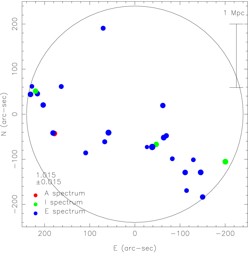
Figure 10: The distribution on the sky of the galaxies with $z=1.015\pm 0.015$ in the region of the HDF. The color coding indicates the galaxy spectral type as in earlier figures. The size of the circle increases with the apparent brightness at $R$ of the galaxy.

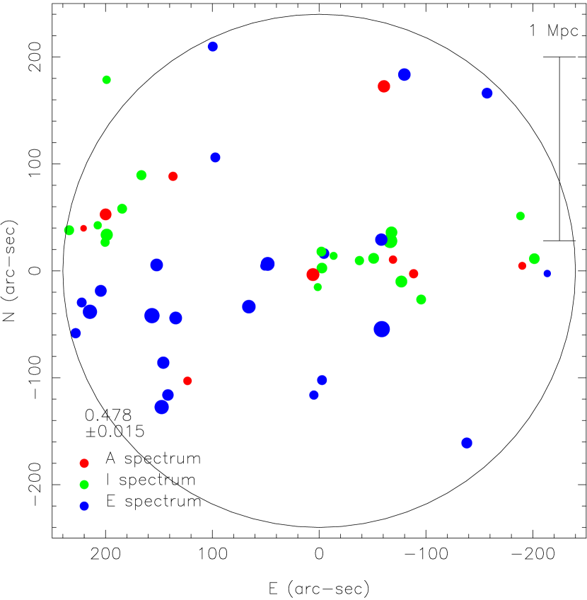
Figure 11: The distribution on the sky of the galaxies with $z=0.478\pm 0.015$ in the region of the HDF. The symbols are identical to those of figure 10.

The field studied here is 8 arcmin in diameter, which corresponds to 3.0 Mpc at $z=0.5$ and to 3.7 Mpc at $z=1$. This means that we can only probe structure at the length scale of groups and clusters, and cannot discern transverse structure at any larger scale. Figures 10 and 11 show the spatial distribution for the highest major redshift peak detected, at $z=1.015$, and for the very populous redshift peak at $z=0.478$. In the case of the latter, the spatial distribution is highly non-uniform; there appear to be two groups $\sim$1.5 Mpc apart. The spatial distribution of galaxies in the peak at $z=1.016$ also appears non-uniform, with a group/cluster centered about 100 arcsec SW of the center of the HDF.

4.3 The Velocity Dispersions of the Strong Redshift Peaks

The velocity dispersions for the sample of statistically significant redshift peaks are listed in Table 6. These have been computed using the biweight algorithm of Beers, Flynn & Gebhardt (1990) because of its resistance to the presence of outliers. The mean and sigma for each structure are calculated from a sample which in general extends over the regime $z_{p}{\pm}0.010$. The instrumental contribution to $\sigma(v)$, estimated to be 200 km s^-1 in the observed frame, has been removed in quadrature. The number of galaxies in each peak is estimated by counting the number within 1$\sigma$ of the peak and assuming Gaussian statistics. Adding up the total estimated membership for the set of statistically significant peaks, we find that 68% of the galaxies are in groups with an maximum overdensity of larger than 3, in agreement with the results from Cohen et al. (1999a) and from our earlier work with a much smaller sample in the HDF (C96).

In most cases the peak finding algorithm was successful in decomposing close peaks into their separate components. This is evident in the region around $z\sim 0.08$ and $z\sim 0.48$. However, the region around $z\sim 0.41$ was manually divided into two separate groups as indicated in the notes to Table 6. These three cases are believed to represent multiple groups within a single redshift peak. Now that we have a much larger sample covering a larger area on the sky it should not be surprising that we find more than one group of galaxies within the same redshift peak.

The very low velocity dispersions achieved in some cases (there are four entries in Table 6 with $\sigma_{v}<200$ km s^-1) is very gratifying and supports the quoted errors of our redshifts.

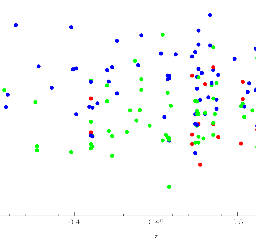
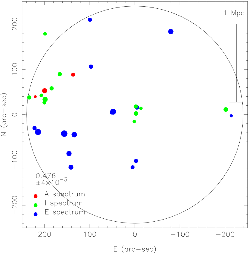
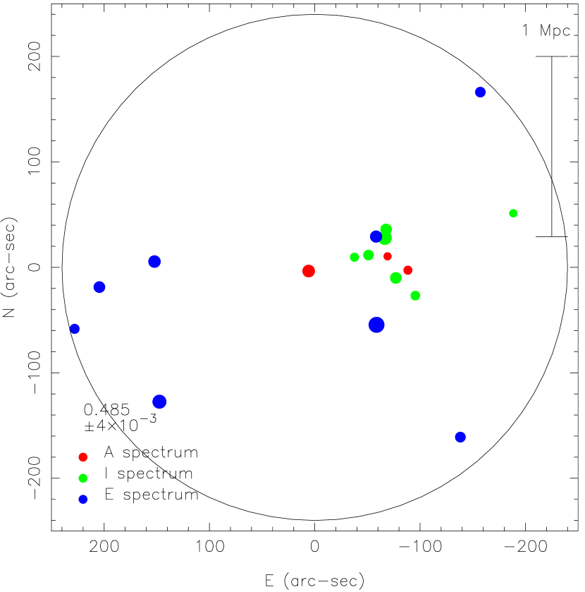
Figure 12: The first panel shows the region $z\sim 0.5$ of the $z$ distribution of Figure 8a in more detail. The second and third panel show the spatial distribution of the galaxies in the two groups that together comprise the redshift peak at $z_{p}=0.478$. The symbols and colors used to denote galaxy spectral types are the same as in Figure 6.

The individual groups contributing to the large redshift peak at $z_{p}=0.48$ can be separated not only in velocity space but also spatially within the area on the sky covered by our survey. The three panels of Figure 12 show first the velocity structure of this redshift regime at even higher resolution than Figure 8 , then present a decomposition of this structure (shown as a whole in Figure 11) into two separate groups with $z_{g}=0.476$ and 0.485. These two groups have a transverse separation of 1.7 Mpc and a difference in mean velocity (in the rest frame) of 350 km s^-1. There is a third smaller group that probably can be split off from the second of these at about the same redshift, $z_{g}=0.474$, with its center close to the center of our field. They may be in the process of merging to form a cluster.

Thus the velocity dispersions within the redshift peaks must be treated with caution. Contributions by multiple groups may artificially inflate their values.

4.4 The Radial Separation of the Redshift Peaks

At this point we introduce an additional assumption that the redshift peaks seen so prominently in our sample represent the intersection of our pencil beam with “walls” resembling those discovered locally from the CFA Survey by de Lapparent, Geller & Huchra (1986). The spatial scale of these “walls” as seen locally is very large. Doroshkevich et al. (1996) finds from the LCRS that most galaxies are in sheets separated by 77 ${\pm}9h^{-1}$ Mpc (128 Mpc in our cosmology). Broadhurst et al. (1990) (see also Willmer et al. 1994) claimed to detect strictly periodic “walls” with a spacing of 213 Mpc in our cosmology out to $z\sim 0.2$ from pencil beam surveys.

The only handle we have with our dataset for the region of the HDF on such large scale structure is to look along the line of sight at the separation of the redshift peaks. We must assume that for most “walls” the area on the sky in our survey is sufficiently large that at least one group or sparse cluster will be located within the area surveyed.

We further assume that the “tilt” in redshift of a “wall” across the area surveyed due to the angle of the sheet of galaxies with respect to the plane of the sky is small (see the formula given in C96), and that the small scale non-flatness of a “wall” (i.e. the velocity dispersion of groups or sparse clusters within a sheet itself) is also small. The latter is known to be true in the Local Universe from analysis of the CFA redshift survey (Dell’Antonio, Geller & Bothun 1996) as well as of the LCRS (Landy et al. 1996, Doroshkevich et al. 1996).

The difference in co-moving coordinates between adjacent redshift peaks from the statistically significant sample in the region of the HDF is given in the penultimate column of Table 6. Figure 12 shows a histogram of these separations, smoothed with a Gaussian with $\sigma=10$ Mpc. The smallest separations listed in Table 6 are presumably group-to-group separations within a single “wall”, so the distribution is displayed both with all the entries listed, and with the separations less than 50 Mpc omitted. The vertical lines on the figure are separated by 68 Mpc. While the distribution of our observed “wall” separations shown in Figure 12 is by no means that of a strictly periodic signal, it does show a characteristic length of approximately 70 Mpc, with a suggestion that some peaks have been missed. This is significantly smaller than is found through the analysis of local redshift surveys as described above. The physical processes that could lead to such a scale being imprinted on the fluctuation spectrum are discussed in Szalay (1999).

We caution that pencil beam surveys can exaggerate large scale structure by emphasizing Fourier components with wave vectors roughly perpendicular to the line of sight (e.g. Kaiser & Peacock 1981).

Between $z=0$ and the maximum redshift at which the redshift peaks can still be discerned in our survey of the region of the HDF ($z\sim 1.2$), changing the adopted cosmology among various currently popular models (ignoring $H_{0}$, which just changes the overall scale) distorts the distance scale by 25%. If one is sure that the peaks are strictly periodic, an incorrect choice of cosmological parameters would produce blurring of the peaks in Figure 12. As has already been suggested by Broadhurst & Jaffe (1999), this effect could in principle be used to determine the cosmological parameters, particularly the cosmological constant, if one knew that the “wall” spacing is strictly periodic and one knew the period.

A more careful analysis of the implications for large scale structure of our sample is planned for the future, including Monte Carlo tests and comparison with pencil beams through large scale cosmological simulations.

4.5 Active Galactic Nuclei

There are three objects with at least one broad emission line characteristic of QSOs in this sample. One is at very high redshift ($z\sim 3.4$). The other two are the brightest objects in the peak at $z\sim 0.96$. These two galaxies, with $L<6L^{*}$, are not luminous enough to be considered classical QSOs and are better designated as broad-lined AGNs. The single QSO in the field studied in Cohen et al. (1999a) with $z$ low enough that the redshift distribution can be determined near $z(QSO)$ is also the brightest galaxy in a strong redshift peak.

Our data support the hypothesis that QSOs/AGNs with $z\gtrsim 0.4$ are in general the brightest objects in populous groups or clusters of galaxies, as discussed for QSOs and radio galaxies with $z<1$ by Yee & Green (1984), see also Yee & Ellingson (1993).

5 Luminosity and Density Evolution

We combine our measured redshifts for galaxies in the region of the HDF with the galaxy models of Poggianti (1997) to convert the observed $R$ magnitudes from H99 into luminosities at $R$ in the rest frame. We use Poggianti’s passive evolution models with the $z=0$ spectral energy distributions of present day ellipticals, Sa and Sc galaxies, assuming them to correspond roughly to our spectral class “${\cal A}$”, “${\cal I}$” and “${\cal E}$” galaxies. A small extinction correction of $A_{R}=0.03$ mag from the maps of Schlegel, Finkbeiner & Davis (1998) has been applied. We use $L_{R}^{*}\equiv-21.75$ mag in our adopted cosmology. This value is extrapolated from the results at $B$ compiled by Binggeli, Sandage & Tammann (1988). We do not consider the very high $z$ regime, where the model galaxy SEDs might be substantially in error due to strong dependences on the details of the star formation history adopted.

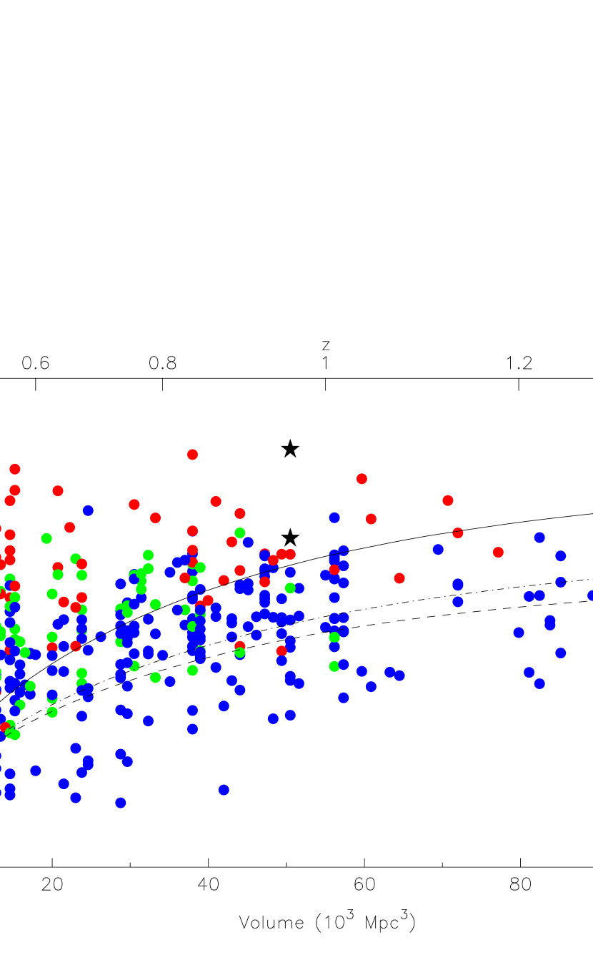
Figure 14: The luminosity $L_{R}$ in units of $L_{R}^{\ast}$ is shown as a function of cosmological volume. The corresponding redshift is shown at the top, while at the right $L_{R}$ is given in units of W. The symbols and colors used to denote galaxy spectral types are the same as in Figure 6. The lines denote the survey cutoff for the HDF Flanking Fields at an apparent magnitude of $R=23$ for elliptical (solid line), Sa and Sc galaxies using the passive evolution models of Poggianti (1997).

Figure 14 displays the luminosity of the galaxies in the region of the HDF in units of $L_{R}^{*}$ as a function of cosmological co-moving volume rather than of redshift. There is no strong increase of $L^{*}$ with $z$. A maximum luminosity of 4$L^{*}$ seems to cover the full range reasonably well, except for $z<0.4$, where the volume sampled is very low and the probability of hitting the brightest galaxies is correspondingly low, and reduced still further as the HDF was selected to be devoid of bright galaxies.

Since this is a nearly complete sample, we can examine Figure 12 to compare the co-moving density of galaxies as a function of $z$. The completeness limit $R=23$ is denoted in Figure 12 for elliptical, Sa and Sc galaxies by a set of curves and it is the area above these curves that must be filled in by either the $\sim$8% of the $R$-selected sample without redshifts or by the EROs that are in this redshift range, but too faint at optical wavelengths to be included in the spectroscopic sample. A forthcoming paper (Cohen et al. 2000) will discuss the luminosity function in detail.

6 The Radio, Mid-IR and Sub-mm Sources in the Region of the HDF

6.1 The Radio Sources

The 8.5 GHz map of Richards et al. (1998) in the region of the HDF is among the deepest ever made with the VLA, and the positional accuracy for radio sources in this map is high. Bearing in mind the probable astrometric accuracy of the optical coordinates, in attempting to find optical counterparts to these radio sources we impose a positional tolerance of 1.0 arcsec for matching the $R$ catalog from H99 with the VLA secure detections with peak flux exceeding 9.0 $\mu$Jy listed in Table 3 of Richards et al.. If we wish to have a probability of less than 5% that a match occurs by chance, the galaxy counts at $R$ imply that we must restrict the candidates for optical counterparts to objects with $R<25.2$.

There are 29 secure VLA sources in the region covered by our redshift survey. Using the positional criteria given above, 15 of these have reasonably bright optical counterparts with redshifts. The difference between the optical and radio positions for these objects, which range from $R=17.7$ to 23.3 mag, has a mean of 0.1 arcsec in RA and the same in Dec, with rms dispersions of 0.4 arcsec in each axis, verifying that the coordinate system of H99 in the Flanking Fields is identical to that of the VLA. There is also one secure identification of a reasonably bright object ($R=23.2$ mag) that does not have a redshift. There are two more possible identifications with bright objects which have positional errors greater than the adopted tolerance but less than 1.5 arcsec.

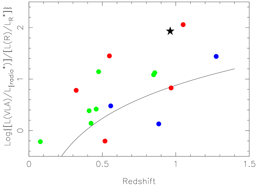
Figure 15: The ratio of the VLA to the optical luminosity is shown as a function of $z$ for the sample of VLA sources of Richards et al. (1998) with peak flux at 8.5 GHz exceeding 9 $\mu$Jy for which a secure optical counterpart with a redshift exists. The optical luminosity is rest frame $R$ in units of $L_{R}^{*}$. The VLA luminosity is in units of $L_{8.5GHz}^{*}$ for local spiral and irregular galaxies with a $K$-correction based on mean spectral index. The symbols and colors used to denote galaxy spectral types are the same as in Figure 6. The curve represents the selection limit imposed by a galaxy with $L=L_{R}^{*}$ and the minimum flux at 8.5 GHz for a secure detection.

We adopt $4.4\times 10^{21}$ W Hz^-1 as the value of the luminosity of a $L^{*}$ spiral or irregular galaxy at 8.5 GHz from the review by Condon (1992). We calculate $K$-corrections for the 8.4 Ghz flux based on a mean radio spectral index of $0.4$ (Richards 2000, see also Fomalont et al. 1991 and Windhorst et al. 1993). We ignore any change in the radio spectral index with $z$ due to normal stellar evolution. We then calculate, for the optical counterparts with measured $z$, the ratio of VLA to optical luminosity, both in units of $L^{*}$. Figure 15 shows this ratio as a function of redshift and it is also included in Table 7. The curve shown in Figure 15 indicates the selection limit imposed by assuming a galaxy with $L_{R}=L_{R}^{*}$ and with a VLA flux at the minimum of that for a secure detection, 9 $\mu$Jy. It produces a reasonably good definition of the lower envelope of the points representing the secure optical identifications.

Details of the identifications are given in Table 7. The first column is the optical ID whose exact coordinates can be found in H99 (or, for objects with spectroscopic redshifts, in Table 2), then the redshift, the galaxy spectral type and the optical luminosity ($L/L_{R}^{*}$). This is followed by the ratio of radio to optical flux, both approximately in units of $L^{*}$ as described above. The last column gives the difference between the VLA coordinates of the radio source and the proposed optical counterpart. If the suggested optical counterpart has no redshift, then instead of the luminosity, the $R$ mag is listed.

For seven of the 29 secure sources detected by the VLA there is no optical counterpart to $R\sim 25$. In addition there are four identifications of radio sources with very faint optical objects with $R\sim 25$ mag, two of which coincide with ISO sources. If the four identifications with very faint objects are correct and these VLA sources, as well as the ones with no optical counterpart at all, are real, then these sources with very faint optical counterparts comprise $\sim$1/3 of the VLA detections at this flux limit. This is in good agreement with the independent result of Richards et al. (2000) using the Hubble Flanking Field catalog of Barger et al. (1999).

We believe that these extremely faint radio sources represent a different class of object, not a continuation of the brighter VLA sources towards somewhat fainter optical and radio flux levels. They cannot simply be more distant or more obscured versions of the sources with optical counterparts as the gap in properties, particularly in the $R$ mag of the optical counterparts, is too large and discontinuous given the small difference in observed radio flux.

However Barger, Cowie & Richards (2000) have recently argued that the rest frame optical IR properties of the radio selected samples are relatively invariant as a function of redshift. They suggest that the faintness of the unidentified galaxies is a consequence of them lying at higher redshifts where the observed frame optical - NIR colors are extremely red and the optical magnitudes faint.

To accomplish this basically requires EROs. Since the secure optical counterparts to the VLA radio sources do not appear to have significant dust content, either there is a discontinuity in their dust content or these galaxies are passively evolving “old” galaxies with $z\sim 1.5$. In the latter case, the radio emission from these weak sources would be decoupled from the current star formation rate in the galaxies.

Barger, Cowie & Richards (2000) discuss the issue of dust at high redshift in more detail.

6.2 The Mid-IR Sources

ISO has surveyed the region of the HDF at 6.5 and at 15$\mu$, with many more sources detected at the latter wavelength. The field of ISO is small, so observing the region of the HDF requires multiple pointings with multiple spatial dithers around each pointing. The observations of Rowan-Robinson et al. (1997) reduced with the algorithms of Aussel et al. (1999) yield 49 sources with a better than 7$\sigma$ detection. Aussel et al. gave redshifts for 29 of these objects compiled from the existing literature. All of these lie at $z<1.24$. They also argued that all of the sources in the HDF proper and all but six of the sources in the Flanking Fields had secure counterparts and that all but one of the 8.4 GHz sources from the VLA survey were seen with ISOCAM.

Even with the 7$\sigma$ detection threshold, the positional uncertainty for ISO sources is worse than with the VLA. When we compound that with the astrometric problems induced by having to tie together multiple pointings, based on Aussel’s evaluation of these uncertainties in the ISO images, we allow a positional tolerance of 2.5 arcsec for matching optical and ISO sources. If we require that the probability that the match occur by chance be less than 5%, the candidate optical counterparts must be brighter than $R=22.8$.

For optical counterparts of ISO sources with a spectroscopic redshift, we compute the emitted luminosity from the observed flux seen by ISO with no $K$-corrections at all and expressed in units of the luminosity of M31 at 12$\mu$, adopting the IRAS flux of 164 Jy (Rice et al. 1988). We denote this by $L_{M31}(ISO)$. The prediction of $K$-corrections for ISO wavelengths is complicated as several different emission mechanisms contribute to the mid-IR luminosity of galaxies. Predictions for starburst galaxies are given by Elbaz et al. (1999); the flux decreases by about a factor of 10 between $z=0$ and $z=1$.

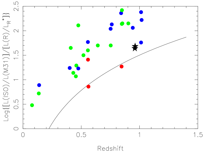
Figure 16: The ratio of the ISO to the optical luminosity is shown as a function of $z$ for the sample of highly significant ISO sources of Aussel et al. (1999) for which a secure optical identification and a redshift exist. The optical luminosity is rest frame $R$ in units of $L_{R}^{*}$. The ISO luminosity is in units of the flux of M31 at 12$\mu$. The symbols and colors used to denote galaxy spectral types are the same as in Figure 6. The curve represents the selection limit imposed by a galaxy with $L=L_{R}^{*}$ and the minimum flux for a secure detection with ISO, taken to be 40 $\mu$Jy. No $K$-correction has been applied to the ISO data.

The results of cross checking the $R$ photometric catalog of H99, our redshift catalog and the ISO detections for the region of the HDF are given in Table 8. The first column is the optical ID whose exact coordinates can be found in H99 (or, for objects with spectroscopic redshifts, in Table 2), then the redshift, the galaxy spectral type and the optical luminosity ($L/L_{R}^{*}$). This is followed by the ratio of emitted ISO to optical flux, $L_{M31}(ISO)/[L_{R}/L_{R}^{*}]$. Then follows the positional difference, whose mean in RA is 0.6 arcsec, with $\sigma=1.2$ arcsec, while the mean difference in Dec is 0.4 arcsec with $\sigma=1.0$ arcsec. Figure 16 plots the ratio of $L(ISO)/L(R)$ with the normalization given above as a function of redshift. The curve shown in Figure 16 indicates the selection limit imposed by assuming a galaxy with $L_{R}=L_{R}^{*}$ and with an observed ISO flux at the minimum of that for a secure detection, 40 $\mu$Jy.

The large apparent mid-IR luminosities of the ISO sources in the region of the HDF should not be a concern. They are normalized to the mid-IR flux of M31, while the IRAS flux at the same wavelength for M82, the nearest luminous galaxy showing signs of a starburst, given in Rice et al. (1988), is 35 times larger.

About 2/3 (32/49) of these ISO sources have secure identifications and redshifts. We confirm all of the redshifts used by Aussel et al. with the exception of C36516_1220 which is at $z=0.401$ rather than $z=0.299$ (see the Appendix). These ISO sources are matched with the brighter galaxies of the sample at moderate redshift. Nine more have probable identifications where either the positional tolerance is within range but the object is fainter than the cutoff of $R=22.8$ or the positional tolerance is slightly higher than the limit. Two of these have matches with positional differences of $2.5<\delta<3.0$ arcsec for an object with $R<22.8$ and in both of these cases there is a fainter object which is even closer to the ISO position. Some of the “probable” matches may be spurious.

There are only 8 of the 49 ISO objects with no suggested optical counterparts to $R=24.5$. The median flux observed with ISO for the unidentified sources is about a factor of 3 smaller than that of the identified sources. A relatively bright optical cutoff ($R=22.8$ mag) has been imposed for secure identifications of ISO sources, mandated by the relatively poor source positions of ISO. Again this is consistent with Aussel et al. who used near IR and optical images and claimed identifications for 43/49 of the sources.

6.3 The Origin of Emission in the Radio and in the Mid-IR in These Galaxies

The total dynamic range of both the ISO and VLA data is not large - a factor of 10 or 20 from the brightest object detected in their HDF maps to the faintest secure detection. Thus there will be a selection effect (i.e. a Malmquist bias) in looking at any property of the ISO or radio sources as a function of $z$ as long as this property has a finite distribution. In particular, as $z$ increases, only the most extreme examples will be picked up by the existing radio or mid-IR surveys. The properties relevant here include luminosity, star formation rate (henceforth SFR), amount of dust and the presence of an AGN or of radio emitting gas in a galaxy’s environment. While a strong AGN will be easily detectable spectroscopically, a weak AGN may not contribute enough optical luminosity to stand out in the total emission from a luminous galaxy, but will make a noticeable difference in the total radio flux of the galaxy. Many such examples exist locally, for example M87.

Elbaz et al. (1999) review the sources of emission in the mid-IR, which are thermal emission from dust, discrete spectral features emitted (and absorbed) by dust, and thermal emission from stars. Although the vertical axis of Figure 16 is not the SFR, it can be translated into such by applying a correction scaling factor for the mean SFR per unit $R$ luminosity appropriate for each of the galaxy spectral classes. Figure 16 does suggest that the mid-IR emission is monotonically increasing with SFR, as expected. Those galaxies whose spectra indicate relatively little ongoing star formation (i.e. spectra dominated by absorption lines) appear to emit relatively less flux at the ISO wavelengths and hence lie at the lower envelope of the distribution shown in Figure 16. The AGNs are faint in the mid-IR while the majority of the optical counterparts to ISO sources have galaxy spectral types indicating some or a lot of ongoing star formation.

As reviewed by Condon (1992), the radio flux for normal galaxies without an active galactic nucleus arises from free-free emission and from synchrotron emission. The radio flux of normal spiral and irregular galaxies is in the mean proportional to their flux at 60$\mu$. The models of Helou & Bicay (1993) tie the radio flux to the SFR through the diffusion of cosmic-ray electrons whose synchrotron emission produces the radio flux. However, there is also the possibility for radio emission from an AGN. Given that we are selecting the very brightest sources at each $z$, this cannot be dismissed.

It is clear from comparing Figure 15 with Figure 16 that radio emission is not well correlated with mid-IR emission for these faint radio sources in the HDF. At least some of the radio sources must arise from weak AGN, as is also the case among the optical counterparts found by Hammer et al. (1995) for the microjansky radio sources in one of the CFRS fields. The two most radio bright galaxies in the region of the HDF are the spectroscopically identified AGN C36463_1404 and the optically luminous object C36443_1133, whose optical spectrum is that of a classical luminous elliptical galaxy and which may be a cD galaxy at high redshift. The latter appears to show spatially extended radio lobes (Richards et al. 1998). Most of the galaxies which are detected VLA sources in the region of the HDF do not show signs of a high current SFR in their spectra.

Machalski & Condon (1999) have searched the NVSS radio database (Condon et al. 1998) for galaxies in the Las Campanas Redshift Survey (Shectman et al. 1996) of the nearby Universe. Approximately one third of the detected radio sources in this flux limited survey appear to arise in AGNs rather than in starbursts or normal galaxies. The AGNs in the mean had a larger ratio of radio to optical flux. It is thus not surprising that the mid-IR emission seen by ISO does not correlate well with the radio flux in the distant sources in the region of the HDF.

To conclude this discussion, we find the fraction of optical counterparts that are in the statistically complete sample of redshift peaks. We use the list of peaks and their velocity dispersions in the rest frame given in Table 6. For the definite identifications of VLA sources, 11 of the 13 optical counterparts with $z<1$ lie within 1.5$\sigma$ of a peak which is a member of the statistically significant sample of redshift peaks. This implies that essentially all these galaxies lie within the peaks. The only very discrepant object (C36414_1142, at 2.9$\sigma$ from the relevant peak) has a very uncertain redshift. (It is also one of the persistent outliers in the photometric redshift comparisons.) For the ISO sources, 26 of the 32 secure optical counterparts have redshifts that are within 1.5$\sigma$ of their respective peak from the statistically complete sample, implying that 30 of the 32 galaxies lie within the statistically complete sample of redshift peaks.

These fractions ($\sim$90% for the VLA and the ISO sample) are even higher than those calculated earlier for the field galaxies (68%). The optical counterparts to the VLA and ISO sources are among the most luminous galaxies in the sample, and so it is not surprising that they show even more clustering that the total sample of field galaxies.

6.4 The SCUBA Sources

Source identification based on the poor resolution and near confusion limited images produced in the sub-mm by SCUBA is a complex problem. In this relatively unexplored wavelength regime we also lack the experience which might guide us in defining characteristics to choose the correct object among the many possible optical candidates within the typical sub-mm positional error circle. The first survey of the HDF in the sub-mm is that of Hughes et al. (1998), who found five sources in a roughly 5 square arcminute region covering the HDF. The identification of these objects has been questioned by Richards (1999), who asserts that the SCUBA positions are systematically shifted on the sky by an amount larger than anticipated by Hughes et al. in their discussion of the accuracy of the SCUBA astrometry. Smail et al. (1999) suggest that at least some faint sub-mm galaxies may be EROs, making a difficult situation even more complex. However, a recent analysis by Barger, Cowie & Richards (2000) of combined 20 cm VLA and SCUBA imaging of the Flanking Fields has shown that the bulk of the SCUBA sources are very faint in the optical and near IR ($I>24$ and $K=21-22$) which would place them beyond the reach of current spectroscopic work.

7 Summary

In this paper we have presented our extensive redshift survey for the HDF and Flanking Fields which contains 671 objects including 610 galaxies and is 92% complete to $R=24$ in the HDF and to $R=23$ in the Flanking Fields within a diameter of 8 arcmin centered on the HDF. A statistically significant sample of redshift peaks was defined using Gaussian kernel smoothing combined with a minimum overdensity threshold. These structures have velocity dispersions typical of groups of galaxies. In some cases, closely spaced redshift peaks can be decomposed into multiple groups of galaxies separated both in redshift and in position on the sky. As we have seen before in C96 and in Cohen et al. (1999a), most ($>68$%) of the galaxies are located in these peaks, which are now apparent out to $z\sim 1.2$. The absorption-line dominated systems preferentially reside in these redshift peaks and are among the most luminous galaxies in them for $z<0.8$.

We interpret the redshift peaks as representing the intersection of the line of sight of the pencil beam with “walls” of galaxies as originally described in the local universe from the CFA Survey by de Lapparent, Geller & Huchra (1986). Since the characteristic size of our field is 3 – 4 Mpc, there is then a fairly large probability that a group or small cluster of galaxies will lie within our field for most of these “walls”. The spacing of the redshift peaks along the line of sight corresponds to the characteristic separation of these large scale structures, which is $\sim$70 Mpc in our adopted cosmology. The results are consistent in general, although not in detail, with other analyses of large redshift surveys in the Local Universe, e.g. the CFA redshift survey (Dell’Antonio, Bothun & Geller 1996) and the LCRS (Landy et al. 1996, Doroshkevich et al. 1996) and with those of Broadhurst et al. (1990), although these groups find the “wall” separation to be somewhat larger than the value we have found. At $z\sim 0.1$ this model is supported by the work of the ESO Slice Project (Vettolani et al. 1997) and at $z\sim 0.3$ by the work of Small et al. (1999). Our survey suggests that these structures originated when the Universe was less than half its present age.

We have found that about 7% of the $K$-selected sample ($K<20$) are extremely red objects with $R-K>5$ and the reddest such has $R-K=6$. One of these has a redshift and is a galaxy at $z\sim 1$ with no detectable current star formation. We suspect that this is typical of all the EROs in this magnitude and color range.

We have searched for optical counterparts of the sources detected with the VLA at 8.5 GHz by Richards et al. (1998). Two thirds of the secure radio sources with observed fluxes at this wavelength exceeding 9 $\mu$Jy can be identified with bright galaxies ($R\sim 21$) at moderate redshift. About 25% of them have no optical counterpart or a very faint one ($R\geq\sim 25$). These appear to be a different population from the first group rather than just a continuation of them in some property such as distance or dust content.

We have also searched for optical counterparts to the ISO sources of Aussel et al. (1999). About 2/3 of these can be identified with bright galaxies ($R\sim 21$ mag) at moderate redshift. Because of the larger positional uncertainty of the ISO astrometry and the high areal density of faint optical objects, the nature of the ISO sources without bright optical counterparts cannot be determined at this time, but is consistent with them mostly being galaxies somewhat fainter than the adopted brightness cutoff.

The presence of emission in the mid-IR appears to be roughly proportional to the rate of ongoing star formation, as would be expected. However, the presence of detectable radio emission is not so tightly coupled to the current star formation rate; a substantial fraction of these radio sources must be weak AGNs.

Both the VLA and the ISO sources appear to be even more clustered than the sample as a whole, with $\sim$90% of them lying within the statistically complete sample of redshift peaks.

We have also used our catalog of redshifts in the region of the HDF to demonstrate that photometric redshift schemes can predict redshifts to high precision (as good as $\sigma=5\%$ in $(1+z)$) for the majority of galaxies with $z<1.3$.

Appendix A Changes to Published Redshifts

The sample of the Lick Deep Group is used as published in Phillips et al. (1997) and Lowenthal et al. (1997) with the addition of one galaxy whose spectrum was obtained in 1996 but no redshift was deduced until early 1999 (H36384_1231). Also data from the setup stars (all of which are relatively bright stars) used to align the slitmasks were incorporated into the redshift table. As communicated to JGC by A. Phillips, the redshift of F36380_0922 (published as $z=0.512$ in Phillips et al. 1997) was changed to $z=0.767$ .

The redshifts given by Steidel et al. (1996) were used as modified and supplemented in the review by Dickinson (1998). Note that one redshift was changed in the latter (H36482_1417, published originally as 2.845 and corrected later to 2.008) and one (H36513_1227) was withdrawn completely.

Several modifications were made to the redshifts published in C96. In most cases, these were not because the features original seen were not really present, but rather because the original interpretation of the features in the spectrum was subsequently shown to be incorrect. The redshift of F36528_1453 was changed when it was realized that the line previously identified as 3727 Å of [OII] is actually the 5007 Å line of [OIII]. The redshift of F36559_1454, which was initially thought to be a late type galactic star, changed when it was realized that the feature originally ascribed to MgH was actually the H+K break. The redshift of F37098_1523 changed when spectra reaching further towards the blue became available which clearly showed the H+K break to be bluer than the spectral coverage of the earlier spectra. The new spectrum indicated that the feature ascribed to the H+K break was actually the Mg triplet region. The redshift of H36446_1227 changed when it was realized that the far-UV interstellar lines had been misidentified initially. The original redshift of H36516_1220 is from a spectrum of low SNR. A better spectrum subsequently obtained by the Hawaii group led to a redetermination of the redshift of this object. In addition to these substantive changes, a small modification was made to the redshift of F36223_1241. Table 9 lists the six corrections to redshifts published in C96 made here.

In addition, there was a case of object confusion in C96 among the pair H36467_1236 and H36470_1236 which has been corrected here.

Updates to the redshifts originally from the Hawaii web site are not listed here. Similarly, some of the redshifts published as preliminary values in Hogg et al. (1998) have been modified; see the notes in the redshift catalog of Table 2.

Appendix B The Objects With $R<24$ in the HDF Without Redshifts

Table 10 lists the eight objects that are present in the photometric survey of H99 with $R<24$, are in the HDF itself, and do not have spectroscopic redshifts at this time. Most of these objects have been observed spectroscopically with the LRIS at Keck Observatory more than once each, and for several hours each time.

NOTE ADDED MAY 17, 2000 – There are two new redshifts for objects in the HDF with $R<24$, H36377_1235 and H36472_1342. The former comes from my continuing observations in this region, while the latter is from S.Dawson, D.Stern, A.J.Bunker, H.Spinrad, & A.Dey (2000, in preparation). There are also two new redshifts for objects with $z\sim 4.5$ from Stern & Spinrad (1999). These four objects are listed in Table 2b, but are not included anywhere else in this paper. A note in press will be added to the published version as well with these new redshifts, although it is probably too late to incorporate them into Table 2b in the paper which will appear shortly in the ApJ.

Table 1: Sources for the Redshifts

Reference	Number Objects	Abbrev.
Previously Published:
Cohen et al. (1996) (Caltech + Hawaii)	140	c96
Phillips et al. (199)+Lowenthal et al. (1997)	129	l96
Steidel et al. (1996) (See also Dickinson 1998)	15	s96
Steidel et al. (1999)	2	s99
Spinrad et al. (1998)	1	spi
Waddington et al. (1999)	1	wad
Weymann et al. (1998)	1	wey
This Paper:
Cohen	$\sim$380	cal
Hawaii	$\sim$150	haw
Steidel	5	st0

Table 2a: Redshift Catalog for the Flanking Fields of the HDF

RA		Dec		$R$	$z$	Quality	Sp.Type	Source	Notes
($-12$h)		($-62^{\circ}$)		(mag)
36	15.90	12	37.3	19.27	0.286	1	$\cal IE$	cal
36	17.60	14	2.2	21.73	0.818	4	$\cal E$	cal
36	17.65	14	8.1	22.55	0.848	4	$\cal E$	cal
36	17.69	13	44.3	20.93	0.534	1	$\cal A$	l96
36	18.70	11	54.1	22.36	0.766	1	$\cal EI$	cal
36	19.41	14	28.7	22.60	0.798	1	$\cal EI$	cal
36	19.47	12	52.5	20.05	0.474	1	$\cal EI$	cal
36	19.50	11	58.9	22.49	0.938	4	$\cal E$	cal
36	19.72	13	53.1	20.36	0.286	1	$\cal I$	cal
36	19.85	12	55.3	24.20	0.695	1	$\cal E$	cal	c
36	19.89	12	51.5	20.30	0.695	1	$\cal EB$	cal	n
36	19.89	13	47.8	20.75	0.535	1	$\cal I$	cal
36	21.03	12	3.8	20.62	0.457	1	$\cal I$	cal
36	21.12	12	7.9	21.80	0.841	1	$\cal E$	cal
36	21.20	13	6.4	21.94	0.474	1	$\cal I$	cal
36	21.27	11	0.5	22.82	0.635	1	$\cal I$	cal
36	21.33	11	9.7	23.56	1.014	1	$\cal I$	haw
36	21.33	14	17.1	20.73	0.520	1	$\cal A$	cal
36	21.57	12	26.8	20.09	0.398	1	$\cal I$	c96
36	21.59	13	0.3	21.14	0.688	1	$\cal I$	cal
36	21.59	11	22.4	22.89	0.639	4	$\cal E$	cal
36	21.73	13	13.5	23.07	0.399	1	$\cal E$	cal
36	22.21	12	37.2	21.86	0.630	1	$\cal IE$	c96
36	22.22	11	6.2	20.83	0.277	1	$\cal I$	cal,haw
36	22.34	12	41.3	20.59	0.458	1	$\cal I$	c96	d
36	22.82	12	59.7	20.38	0.472	1	$\cal A$	c96
36	22.98	14	31.0	21.22	0.190	1	$\cal I$	cal
36	23.06	13	46.3	20.71	0.485	1	$\cal IE$	c96
36	24.02	11	9.6	22.46	0.766	1	$\cal EI$	cal
36	24.16	15	14.4	23.14	0.222	1	$\cal E$	cal
36	24.31	15	25.3	22.78	0.682	1	$\cal I$	cal
36	24.41	14	54.1	20.34	0.628	1	$\cal I$	l96,cal
36	24.44	14	48.0	22.48	0.582	1	$\cal EI$	cal
36	24.54	11	39.3	21.01	0.231	1	$\cal EI$	cal,haw
36	24.55	11	11.2	22.05	0.748	4	$\cal E$	cal,haw
36	24.68	14	18.7	24.17	1.450	4	$\cal E$	haw
36	24.71	15	10.4	20.41	0.641	1	$\cal A$	cal
36	24.91	14	38.7	21.59	0.642	1	$\cal A$	cal
36	24.95	12	52.1	22.76	0.631	1	$\cal A$	cal,haw
36	25.07	13	41.8	24.32	0.654	1	$\cal E$	l96
36	25.08	13	0.5	20.73	0.518	1	$\cal A$	c96
36	25.20	14	10.7	23.30	0.318	1	$\cal EI$	l96
36	25.36	12	35.2	22.83	0.526	3	$\cal A$	haw,cal
36	25.43	14	4.8	17.43	0.000	1	$\cal M$	cal,haw
36	25.45	15	19.6	21.82	0.642	1	$\cal E$	cal
36	25.99	14	11.4	23.51	0.528	1	$\cal E$	l96
36	26.63	12	52.0	20.66	0.557	1	$\cal I$	c96
36	26.66	10	19.4	22.87	0.256	1	$\cal E$	cal
36	27.07	15	9.4	21.60	0.794	1	$\cal AI$	cal
36	27.10	10	1.1	21.53	0.842	1	$\cal EA$	cal
36	27.25	13	42.3	21.43	0.000	1	$\cal M$	l96,cal,haw
36	27.31	12	57.9	22.28	1.221	1	$\cal EI$	l96,haw
36	27.46	10	17.6	20.59	0.253	1	$\cal I$	cal
36	27.53	15	41.2	21.98	0.487	1	$\cal EI$	cal
36	27.55	14	18.8	22.37	0.751	4	$\cal E$	cal
36	27.82	12	40.6	21.31	0.519	1	$\cal A$	l96,haw
36	27.88	11	24.1	21.37	0.519	1	$\cal I$	cal,haw
36	27.89	14	49.0	21.64	0.680	1	$\cal I$	cal
36	27.97	11	22.0	22.78	0.925	4	$\cal E$	cal	c
36	28.04	15	7.4	21.60	0.440	1	$\cal I$	cal
36	28.24	14	32.8	21.06	0.243	1	$\cal E$	cal,haw
36	28.26	12	37.5	21.33	0.518	1	$\cal I$	c96
36	28.43	10	37.0	22.76	0.760	1	$\cal E$	l96
36	28.53	9	51.4	23.07	1.016	4	$\cal E$	cal	e
36	28.54	9	53.3	24.34	1.216	4	$\cal E$	cal	e
36	28.72	10	23.3	22.11	0.936	5	$\cal E$	cal
36	28.73	13	57.8	23.05	0.639	1	$\cal I$	haw
36	28.80	12	39.3	24.00	0.880	1	$\cal E$	l96
36	29.01	13	46.6	23.02	0.693	1	$\cal E$	l96,haw
36	29.07	13	52.1	23.27	1.398	4	$\cal E$	haw
36	29.13	11	53.0	22.62	0.530	1	$\cal E$	cal
36	29.14	10	46.0	23.50	1.013	4	$\cal E$	haw
36	29.68	14	20.6	22.59	1.055	3	$\cal A$	cal
36	29.70	13	25.0	23.25	0.758	1	$\cal E$	haw
36	29.77	13	29.7	23.03	0.748	1	$\cal EI$	cal,haw
36	29.91	14	40.9	22.81	0.762	1	$\cal IE$	cal
36	29.98	14	3.1	21.97	0.793	1	$\cal I$	c96
36	30.03	12	24.2	22.67	0.410	1	$\cal I$	c96
36	30.24	10	14.0	22.06	0.482	1	$\cal EI$	l96
36	30.38	15	58.6	22.55	0.232	1	$\cal EI$	cal
36	30.39	15	2.3	22.84	0.000	1	$\cal M$	cal
36	30.42	12	8.5	20.71	0.456	1	$\cal I$	c96
36	30.62	15	33.7	22.07	0.530	1	$\cal EI$	cal
36	30.77	10	58.7	20.55	0.295	1	$\cal I$	cal
36	30.87	14	33.4	21.23	0.438	1	$\cal IE$	l96
36	30.98	15	27.8	20.88	0.000	1	$\cal M$	cal
36	31.20	12	36.3	21.35	0.455	1	$\cal E$	haw
36	31.47	11	13.9	22.09	1.013	1	$\cal EA$	cal
36	31.62	16	4.0	21.39	0.784	1	$\cal I$	cal
36	31.90	12	40.4	21.51	0.528	1	$\cal EI$	c96
36	32.01	10	20.4	22.66	0.316	1	$\cal I$	cal
36	32.02	12	24.8	24.59	0.398	1	$\cal EI$	haw
36	32.43	10	37.6	19.97	0.136	1	$\cal I$	cal
36	32.47	11	5.1	19.67	0.518	1	$\cal A$	cal
36	32.47	15	13.2	21.97	0.684	1	$\cal I$	cal
36	32.55	11	13.3	22.51	0.518	1	$\cal A$	cal
36	32.71	12	39.2	22.84	0.458	1	$\cal EI$	haw
36	32.77	12	43.8	21.45	0.562	1	$\cal I$	c96
36	33.16	15	13.8	21.92	0.521	1	$\cal IE$	cal
36	33.17	11	34.0	20.25	0.080	1	$\cal E$	c96
36	33.21	12	35.6	23.11	1.140	4	$\cal E$	haw
36	33.25	14	11.0	23.62	1.344	4	$\cal E$	l96
36	33.44	14	32.3	23.08	0.748	1	$\cal E$	l96
36	33.51	14	18.0	23.91	3.408	6	$\cal Q$	haw
36	33.60	13	19.8	21.78	0.845	1	$\cal I$	l96,haw
36	33.62	10	5.6	22.15	1.015	1	$\cal EI$	cal
36	33.70	14	31.0	20.89	0.519	1	$\cal I$	l96
36	33.76	11	56.4	21.76	0.459	1	$\cal IE$	l96,haw
36	33.99	16	4.6	22.60	0.835	4	$\cal E$	cal
36	34.00	10	54.4	21.55	0.762	1	$\cal EI$	cal
36	34.06	10	45.8	23.25	1.011	4	$\cal E$	cal
36	34.17	13	57.8	19.14	0.000	1	$\cal S$	l96,cal,haw
36	34.17	13	5.8	24.24	0.847	4	$\cal E$	haw
36	34.26	14	48.3	22.57	0.507	1	$\cal E$	l96
36	34.28	14	33.0	20.29	0.520	1	$\cal A$	cal
36	34.36	13	12.5	23.15	0.845	1	$\cal IE$	haw
36	34.46	12	13.2	18.84	0.458	1	$\cal I$	cal,haw
36	34.50	14	29.7	22.50	0.519	1	$\cal EI$	cal
36	34.56	12	40.9	23.18	1.219	4	$\cal E$	c96
36	34.84	16	28.3	22.76	0.847	1	$\cal EI$	cal
36	34.91	15	48.6	22.59	0.337	1	$\cal E$	cal
36	34.97	12	24.1	19.63	0.562	1	$\cal A$	c96
36	35.07	14	29.4	22.83	0.297	1	$\cal EI$	cal
36	35.29	15	47.4	22.58	0.336	1	$\cal I$	cal
36	35.30	11	9.7	20.80	0.410	1	$\cal A$	l96
36	36.28	13	19.8	22.20	0.680	1	$\cal EI$	c96
36	36.29	15	0.7	23.03	0.559	1	$\cal E$	cal	j
36	36.35	12	28.2	21.46	0.486	1	$\cal I$	cal
36	36.40	12	37.3	22.94	0.961	4	$\cal E$	cal
36	36.50	13	40.7	21.58	0.558	1	$\cal A$	c96
36	36.59	15	24.5	22.86	0.744	1	$\cal B$	cal
36	36.65	13	46.6	20.32	0.960	6	$\cal Q$	l96,haw	c
36	36.76	11	56.0	21.81	0.557	1	$\cal I$	cal,haw
36	36.79	12	13.1	20.86	0.846	1	$\cal A$	cal,haw
36	36.86	11	34.8	17.66	0.078	1	$\cal I$	c96
36	36.86	12	33.1	23.38	0.437	1	$\cal I$	l96,cal
36	36.88	13	45.7	21.20	0.846	4	$\cal E$	l96	c
36	37.04	11	59.5	21.56	0.779	1	$\cal IE$	cal,haw
36	37.36	12	52.3	21.10	0.485	1	$\cal A$	c96
36	37.62	12	40.7	20.51	0.458	1	$\cal EI$	c96
36	37.63	14	53.5	24.11	0.000	1	$\cal M$	haw
36	37.80	11	49.4	22.72	0.838	1	$\cal A$	c96
36	37.97	9	22.0	21.43	0.767	1	$\cal I$	l96	d
36	37.97	16	15.2	21.36	0.531	1	$\cal A$	cal
36	38.03	9	27.7	23.21	0.513	1	$\cal E$	l96
36	38.13	11	16.2	22.20	1.018	4	$\cal E$	cal
36	38.14	9	53.3	21.04	0.512	1	$\cal EI$	cal
36	38.20	16	4.9	22.27	0.855	1	$\cal I$	cal
36	38.29	11	50.8	22.74	0.842	1	$\cal EI$	cal,haw
36	38.36	9	53.0	21.46	0.000	1	$\cal M$	cal
36	38.38	15	39.5	22.85	0.000	3	$\cal S$	cal
36	38.48	13	12.9	22.27	0.635	1	$\cal E$	cal
36	38.60	15	58.6	22.94	0.478	1	$\cal EI$	cal
36	38.63	13	38.9	22.32	0.357	1	$\cal I$	cal
36	38.63	14	21.6	23.66	2.990	1	$\cal EA$	l96
36	38.67	15	10.1	23.61	0.462	1	$\cal E$	l96
36	38.76	15	47.1	22.28	0.904	1	$\cal EA$	cal
36	38.86	11	28.6	23.64	0.453	1	$\cal E$	haw
36	38.87	12	57.1	22.28	1.127	2	$\cal EA$	cal,haw
36	38.90	11	18.6	22.53	0.934	4	$\cal E$	cal
36	38.93	9	11.5	22.61	0.342	2	$\cal A$	cal
36	39.00	12	45.0	22.58	0.487	1	$\cal I$	cal
36	39.06	10	6.1	21.22	0.635	1	$\cal I$	cal
36	39.22	16	23.4	23.20	0.850	2	$\cal A$	cal
36	39.28	15	52.1	23.28	0.521	1	$\cal EI$	cal
36	39.68	10	9.7	21.59	0.509	1	$\cal I$	l96
36	39.70	15	26.2	20.30	0.377	1	$\cal I$	cal
36	39.75	15	47.7	22.04	0.848	2	$\cal A$	cal
36	39.82	9	53.7	25.00	0.748	4	$\cal E$	cal
36	39.83	10	1.7	22.05	0.137	1	$\cal B$	l96
36	39.92	12	50.0	21.53	0.848	1	$\cal I$	cal
36	39.95	10	29.2	22.59	0.935	4	$\cal E$	cal
36	40.12	13	5.5	20.63	0.488	1	$\cal A$	cal
36	40.32	13	31.0	22.51	0.484	1	$\cal I$	cal,haw
36	40.49	13	22.9	23.87	0.485	1	$\cal I$	l96
36	40.50	10	3.3	22.39	0.749	1	$\cal I$	cal
36	40.52	14	3.6	23.88	1.483	4	$\cal E$	haw
36	40.88	10	54.7	22.61	0.875	1	$\cal E$	cal
36	41.02	15	0.7	22.92	0.000	1	$\cal M$	l96
36	41.05	9	48.8	20.38	0.410	1	$\cal I$	cal
36	41.13	13	14.3	23.08	1.017	1	$\cal E$	cal	j
36	41.17	14	21.0	21.41	0.519	1	$\cal I$	cal
36	41.33	15	47.6	22.85	0.472	8	$\cal A$	cal
36	41.47	14	2.7	20.85	0.557	1	$\cal A$	l96
36	41.53	9	2.9	22.31	0.713	4	$\cal E$	cal
36	41.56	9	48.1	20.40	0.518	1	$\cal AI$	cal
36	41.68	13	24.2	22.87	0.488	1	$\cal EI$	cal
36	41.74	9	43.3	22.51	0.845	1	$\cal A$	l96
36	42.04	13	21.2	23.95	0.846	4	$\cal E$	cal
36	42.05	13	32.3	$>26.0$	4.424	11	$\cal E$	wad	m
36	42.16	15	45.2	21.61	0.857	1	$\cal I$	cal
36	42.41	12	52.2	23.58	1.237	4	$\cal E$	haw
36	42.51	15	42.7	22.61	2.450	3	$\cal A$	cal
36	42.53	9	33.8	20.72	0.530	1	$\cal I$	cal
36	42.55	11	21.9	23.03	0.845	1	$\cal EI$	l96
36	42.55	15	18.4	21.79	0.533	1	$\cal EI$	cal
36	42.71	13	6.7	22.02	0.485	1	$\cal I$	cal
36	42.73	15	2.7	23.17	0.698	1	$\cal EI$	cal
36	43.01	10	30.2	21.82	0.551	1	$\cal E$	cal
36	43.03	16	31.9	22.46	0.870	4	$\cal E$	cal
36	43.04	16	36.0	24.64	3.368	11	$\cal E$	cal	l
36	43.12	11	8.5	22.48	0.299	1	$\cal I$	cal
36	43.50	15	32.2	22.82	0.847	1	$\cal E$	l96
36	43.52	16	24.9	21.78	0.161	1	$\cal AI$	cal
36	43.75	13	56.7	20.65	0.201	1	$\cal IE$	c96
36	43.82	9	21.7	20.58	0.000	1	$\cal M$	l96,cal
36	44.04	9	42.9	20.52	0.000	1	$\cal M$	cal
36	44.12	11	23.0	22.87	0.000	1	$\cal M$	cal
36	44.14	14	59.2	21.72	0.000	1	$\cal M$	cal
36	44.27	15	18.2	22.54	0.570	1	$\cal EI$	l96
36	44.38	10	36.7	22.76	0.890	4	$\cal E$	cal
36	44.48	10	17.9	22.91	0.518	1	$\cal I$	cal
36	44.61	9	26.6	21.46	0.518	1	$\cal I$	cal
36	44.61	13	4.6	21.14	0.485	1	$\cal I$	l96
36	44.67	10	32.3	21.82	0.000	1	$\cal S$	cal
36	44.80	14	55.2	22.97	0.845	1	$\cal EI$	cal
36	44.94	16	16.6	21.88	0.748	1	$\cal I$	cal
36	45.41	13	25.8	22.33	0.441	1	$\cal IE$	cal
36	45.42	15	23.0	22.06	0.683	1	$\cal E$	cal
36	45.86	13	25.7	20.71	0.321	1	$\cal I$	cal,haw
36	45.97	11	1.2	22.77	0.936	4	$\cal E$	l96
36	46.22	15	27.3	22.11	0.851	1	$\cal E$	l96
36	46.31	16	14.5	21.73	0.504	1	$\cal EI$	cal
36	46.32	16	29.2	20.40	0.502	1	$\cal A$	cal
36	46.78	16	36.5	17.65	0.000	1	$\cal M$	l96,cal
36	46.84	10	20.1	22.91	0.170	1	$\cal I$	cal
36	46.84	15	40.6	22.23	0.912	1	$\cal EA$	cal
36	46.86	14	47.1	21.00	0.558	1	$\cal A$	l96
36	46.94	9	6.6	23.84	0.905	1	$\cal E$	l96
36	47.28	16	28.3	21.69	0.873	1	$\cal A$	l96
36	47.38	16	20.3	21.74	0.502	1	$\cal I$	cal
36	47.76	15	12.7	21.43	0.534	1	$\cal IE$	cal
36	47.80	10	45.6	23.43	1.187	3	$\cal A$	cal
36	48.12	11	2.2	22.58	0.650	1	$\cal EI$	cal
36	48.14	15	8.2	24.10	0.426	3	$\cal E$	cal	c
36	48.15	15	24.9	23.05	0.535	4	$\cal E$	cal
36	48.18	10	2.5	21.92	0.682	1	$\cal EI$	cal
36	48.28	15	7.4	22.38	0.890	3	$\cal A$	cal
36	48.48	15	40.4	22.26	0.506	4	$\cal E$	cal
36	48.58	9	32.1	21.06	0.518	1	$\cal I$	cal
36	48.60	15	52.4	21.95	0.347	1	$\cal A$	cal
36	48.61	11	41.1	22.21	0.962	4	$\cal E$	c96
36	48.74	9	42.8	19.20	0.000	1	$\cal M$	l96,cal
36	48.84	15	2.4	24.66	0.364	3	$\cal EI$	cal
36	49.03	15	12.1	22.72	0.457	1	$\cal EI$	l96
36	49.04	16	20.6	22.19	1.300	3	$\cal A$	cal
36	49.46	14	56.5	24.36	0.341	5	$\cal E$	cal
36	49.62	11	12.8	21.47	0.475	1	$\cal EI$	l96
36	49.65	15	34.2	22.80	0.254	1	$\cal I$	cal
36	49.93	10	58.6	22.63	0.684	1	$\cal I$	cal
36	49.94	9	35.4	22.57	0.285	1	$\cal EI$	cal
36	49.95	16	37.1	21.36	0.504	1	$\cal I$	l96
36	50.23	16	16.2	22.62	0.503	1	$\cal A$	l96
36	50.27	11	27.4	22.88	0.954	1	$\cal EI$	cal
36	50.71	10	58.8	21.11	0.474	1	$\cal EI$	c96
36	50.99	11	34.3	22.14	0.000	1	$\cal M$	cal
36	51.07	9	38.6	21.27	0.205	1	$\cal E$	cal
36	51.09	10	30.9	20.23	0.410	1	$\cal I$	c96,l96
36	51.61	9	54.5	21.18	0.136	1	$\cal EI$	l96
36	51.64	10	52.3	23.03	0.518	1	$\cal EI$	cal
36	51.84	11	25.4	21.62	0.919	4	$\cal E$	cal
36	52.11	14	57.0	21.71	0.358	1	$\cal EI$	c96
36	52.29	9	31.8	22.64	0.230	1	$\cal E$	cal
36	52.30	15	37.0	22.74	0.936	2	$\cal A$	cal
36	52.37	10	19.9	22.23	0.457	1	$\cal I$	cal
36	52.43	16	37.8	22.78	0.515	1	$\cal E$	cal
36	52.44	10	35.7	21.57	0.321	1	$\cal EI$	c96
36	52.49	9	19.6	22.81	0.954	9	$\cal A$	cal
36	52.75	14	53.3	23.80	0.080	4	$\cal E$	c96	c,e
36	52.86	14	43.9	18.93	0.322	1	$\cal A$	c96,l96
36	52.87	14	53.7	22.02	0.089	1	$\cal IE$	c96	d,e
36	52.93	16	42.0	24.06	0.558	1	$\cal E$	cal
36	52.94	15	45.6	24.31	2.426	11	$\cal E$	cal
36	52.99	15	8.6	22.84	0.942	1	$\cal EI$	l96
36	53.20	11	16.9	22.08	0.942	1	$\cal E$	cal,haw
36	53.43	11	40.3	23.26	1.275	1	$\cal EA$	cal,haw
36	53.55	15	24.8	18.08	0.000	1	$\cal S$	c96
36	53.90	16	6.9	22.84	0.851	1	$\cal EI$	cal
36	54.02	10	46.3	22.68	0.594	1	$\cal EB$	l96
36	54.13	15	14.9	22.84	0.849	1	$\cal E$	cal
36	54.36	14	34.2	22.15	0.577	1	$\cal E$	c96
36	54.57	10	14.6	23.86	0.224	1	$\cal E$	l96
36	54.61	11	27.2	20.58	0.253	1	$\cal I$	cal
36	54.83	15	57.2	22.51	1.132	2	$\cal A$	cal
36	55.28	9	12.6	22.49	0.420	1	$\cal I$	cal
36	55.57	11	35.6	22.32	0.559	4	$\cal E$	cal
36	55.70	9	17.4	20.85	0.421	1	$\cal I$	cal
36	55.80	9	25.4	21.92	0.420	1	$\cal I$	l96
36	55.91	11	40.8	22.56	0.312	1	$\cal A$	cal
36	55.98	14	54.5	21.48	0.321	1	$\cal A$	cal	d
36	56.39	12	9.3	23.22	0.321	1	$\cal E$	c96
36	56.49	14	19.7	20.71	0.106	1	$\cal E$	cal,haw
36	57.49	12	11.0	21.10	0.665	1	$\cal A$	cal,haw	e
36	57.51	12	12.1	22.62	0.561	1	$\cal E$	cal	e
36	57.57	14	37.7	22.51	0.266	1	$\cal EI$	cal
36	57.76	14	54.8	22.49	0.849	1	$\cal I$	cal
36	57.83	12	10.1	22.91	0.971	1	$\cal EI$	cal	c
36	57.83	14	17.9	22.16	0.000	1	$\cal M$	cal
36	57.85	10	12.8	22.02	0.410	1	$\cal A$	l96
36	58.06	11	37.8	23.00	0.681	1	$\cal E$	cal	j
36	58.26	9	23.1	22.05	0.530	1	$\cal I$	cal
36	58.30	9	58.1	17.44	0.137	1	$\cal E$	cal
36	58.35	12	14.1	23.79	1.020	4	$\cal E$	c96
36	58.36	15	48.6	20.94	0.457	1	$\cal B$	c96
36	58.36	14	58.4	24.60	3.382	11	$\cal E$	cal
36	58.37	9	35.4	16.85	0.000	1	$\cal S$	cal
36	58.70	14	38.3	22.38	0.512	1	$\cal EI$	c96
36	58.76	16	37.8	19.47	0.299	1	$\cal I$	c96
36	58.82	14	34.8	20.85	0.678	1	$\cal I$	c96
36	58.96	12	8.8	22.32	0.853	1	$\cal I$	cal
36	59.44	14	4.5	19.56	0.089	1	$\cal EI$	cal
36	59.54	11	53.9	22.54	1.021	1	$\cal EI$	cal,haw
36	59.89	14	49.8	21.62	0.762	1	$\cal EI$	c96
37	0.04	16	5.7	22.46	1.013	1	$\cal EA$	cal
37	0.36	16	16.9	22.33	0.913	1	$\cal EI$	cal
37	0.51	14	5.8	20.67	0.423	1	$\cal I$	c96,l96
37	0.73	11	7.3	22.94	0.801	1	$\cal EI$	cal
37	0.74	11	36.3	24.41	0.000	3	$\cal M$	l96,haw
37	0.85	11	29.3	21.25	0.000	1	$\cal M$	cal
37	1.07	13	19.7	22.62	0.410	1	$\cal E$	cal
37	1.23	12	13.3	24.30	1.516	4	$\cal E$	haw
37	1.44	11	35.7	22.05	0.594	1	$\cal EI$	l96
37	1.51	11	29.0	21.45	0.779	1	$\cal IE$	cal,haw
37	1.57	11	46.6	25.30	0.884	1	$\cal E$	haw	c,m
37	1.67	12	26.0	23.95	0.973	4	$\cal E$	cal
37	1.77	11	44.0	22.10	0.744	4	$\cal E$	cal
37	1.87	16	21.8	22.51	0.310	8	$\cal A$	cal
37	1.91	10	24.6	20.68	0.411	1	$\cal I$	cal
37	1.92	15	10.3	22.20	0.938	1	$\cal EI$	c96
37	1.93	9	39.0	22.48	0.750	1	$\cal EI$	cal
37	1.94	12	25.5	24.93	3.408	11	$\cal E$	cal
37	2.00	11	22.9	18.72	0.136	1	$\cal I$	l96,cal
37	2.00	13	23.0	20.69	0.410	1	$\cal EI$	l96,cal,haw
37	2.03	13	48.8	22.32	0.511	1	$\cal E$	cal,haw
37	2.07	15	17.3	23.56	0.744	1	$\cal E$	l96
37	2.24	12	43.2	22.54	0.104	1	$\cal I$	cal,haw
37	2.37	9	21.9	21.96	0.000	1	$\cal M$	cal
37	2.49	13	42.0	21.25	0.559	1	$\cal EI$	c96
37	2.54	14	48.4	22.38	0.558	1	$\cal AI$	l96
37	2.60	12	16.6	24.04	1.073	4	$\cal E$	haw
37	2.67	13	47.2	23.16	0.513	1	$\cal E$	c96
37	2.71	15	43.5	19.47	0.514	1	$\cal I$	c96
37	2.73	14	1.7	22.60	1.243	4	$\cal E$	c96
37	2.77	16	36.7	23.18	0.378	1	$\cal E$	cal
37	2.81	11	10.4	21.60	0.560	1	$\cal I$	l96
37	2.89	14	23.7	20.27	0.512	1	$\cal I$	c96
37	2.92	14	27.6	23.67	0.898	1	$\cal E$	l96
37	3.27	14	17.8	20.90	0.512	1	$\cal A$	l96
37	3.34	16	31.8	22.16	0.359	1	$\cal E$	cal
37	3.50	11	2.0	21.48	0.518	1	$\cal I$	cal
37	3.52	10	48.4	22.20	0.426	1	$\cal EI$	cal
37	3.80	13	53.1	21.63	0.745	1	$\cal EI$	c96
37	3.82	10	59.7	24.63	2.956	11	$\cal E$	cal
37	3.87	10	9.4	21.85	0.322	1	$\cal IE$	cal
37	3.90	14	41.1	21.48	0.475	1	$\cal EI$	c96
37	4.00	15	23.2	21.89	0.376	1	$\cal I$	c96
37	4.20	12	39.6	23.16	0.861	3	$\cal A$	cal
37	4.24	16	24.8	21.45	0.474	1	$\cal EI$	c96
37	4.50	10	3.8	20.99	0.230	1	$\cal IE$	cal
37	4.61	14	16.0	23.97	1.050	1	$\cal E$	l96
37	4.62	14	29.1	20.96	0.561	1	$\cal I$	c96
37	4.64	10	28.6	21.69	0.411	1	$\cal E$	cal
37	4.78	14	54.8	20.56	0.000	1	$\cal S$	c96,l96
37	5.15	12	10.8	22.41	0.386	1	$\cal EI$	c96
37	5.02	15	46.9	22.77	0.532	1	$\cal EI$	c96
37	5.57	11	29.2	22.37	1.001	4	$\cal E$	cal
37	5.70	13	3.3	21.75	0.109	1	$\cal E$	l96,haw
37	5.75	15	25.1	21.84	0.503	1	$\cal I$	c96
37	5.81	13	17.2	21.95	0.753	1	$\cal EI$	cal
37	5.83	14	23.4	22.48	0.970	1	$\cal E$	haw
37	5.84	11	53.8	21.22	0.904	1	$\cal I$	l96,haw
37	6.00	12	57.9	22.48	0.000	1	$\cal M$	cal
37	6.19	13	32.7	21.85	0.753	1	$\cal IE$	l96,haw
37	6.27	15	17.7	22.22	0.840	1	$\cal EB$	l96,cal
37	6.40	13	14.0	21.78	0.000	1	$\cal S$	cal,haw
37	6.41	15	21.5	22.38	0.513	1	$\cal I$	cal
37	6.44	9	45.3	22.16	0.000	1	$\cal M$	cal
37	6.54	15	12.5	22.94	0.840	4	$\cal E$	cal
37	6.89	9	59.8	21.59	0.434	1	$\cal I$	cal
37	6.91	14	29.5	20.58	0.000	1	$\cal S$	c96
37	6.93	12	8.0	24.13	0.693	1	$\cal E$	l96
37	7.23	11	57.8	22.46	0.593	1	$\cal I$	c96
37	7.25	12	14.1	22.19	0.655	1	$\cal A$	c96
37	7.41	10	15.5	22.86	0.000	1	$\cal M$	cal
37	7.42	13	56.7	23.65	0.752	1	$\cal EI$	haw
37	7.62	11	12.1	20.72	0.472	1	$\cal A$	l96
37	7.75	11	37.7	22.41	0.557	4	$\cal E$	cal
37	7.84	16	5.7	21.88	0.936	1	$\cal EI$	c96
37	7.87	16	2.0	22.66	0.514	1	$\cal EI$	cal
37	8.00	14	44.5	22.26	0.570	1	$\cal E$	l96
37	8.08	12	46.8	21.80	0.654	1	$\cal EI$	l96,haw
37	8.12	14	22.6	19.96	0.563	1	$\cal A$	l96,haw
37	8.13	15	2.0	22.65	0.570	3	$\cal I$	l96
37	8.16	12	15.3	22.06	0.594	1	$\cal EI$	l96
37	8.29	10	56.1	19.96	0.423	1	$\cal I$	cal
37	8.31	12	52.5	22.20	0.838	1	$\cal I$	c96
37	8.33	13	20.8	22.86	0.785	4	$\cal E$	c96
37	8.34	14	53.9	21.88	0.564	1	$\cal EI$	c96
37	8.36	15	14.6	21.62	0.839	1	$\cal EI$	c96
37	8.62	10	51.2	20.66	0.411	1	$\cal EB$	cal
37	8.65	15	1.4	21.68	0.570	1	$\cal I$	c96
37	8.66	11	28.5	22.23	0.907	1	$\cal E$	l96
37	8.66	16	11.6	20.53	0.000	1	$\cal M$	c96	i
37	8.75	12	57.9	23.51	2.269	3	$\cal A$	l96
37	8.83	12	14.4	23.90	0.788	1	$\cal E$	l96
37	8.88	11	17.9	23.05	0.639	1	$\cal I$	haw
37	8.95	12	2.2	22.90	0.855	1	$\cal EI$	c96
37	9.20	12	10.9	23.09	0.476	1	$\cal E$	l96
37	9.50	14	49.1	23.04	0.420	1	$\cal EI$	l96
37	9.51	12	34.5	14.69	0.000	1	$\cal S$	cal
37	9.56	14	23.4	21.10	0.476	1	$\cal A$	c96,l96
37	9.61	10	55.2	23.16	0.858	4	$\cal E$	haw
37	9.85	15	23.9	19.00	0.201	1	$\cal A$	c96	d
37	9.91	10	8.1	22.73	0.000	3	$\cal M$	cal
37	10.24	10	58.9	22.38	0.475	1	$\cal EI$	l96
37	10.36	13	19.7	21.87	0.320	1	$\cal I$	c96	f
37	10.56	11	41.0	21.20	0.789	1	$\cal I$	cal,haw
37	10.58	13	41.6	22.40	0.747	1	$\cal EI$	cal,haw
37	10.79	14	31.5	22.39	0.677	3	$\cal A$	l96,cal
37	10.80	12	0.8	19.83	0.000	1	$\cal M$	l96,cal,haw
37	10.86	11	29.1	22.80	0.475	1	$\cal E$	cal
37	10.91	10	59.0	24.25	0.747	1	$\cal EI$	l96,cal
37	11.08	10	47.6	23.93	0.483	1	$\cal E$	l96
37	11.36	15	45.1	22.43	0.692	4	$\cal E$	cal
37	11.46	10	55.3	22.44	0.855	4	$\cal E$	cal
37	11.58	11	26.5	21.72	0.409	1	$\cal EI$	haw
37	11.59	10	42.4	21.97	0.778	4	$\cal E$	cal
37	11.75	13	0.5	23.05	0.485	1	$\cal E$	haw
37	11.79	15	14.6	19.82	0.299	1	$\cal EI$	cal
37	11.81	10	19.5	21.85	0.414	1	$\cal E$	cal
37	12.38	12	13.1	24.47	0.476	1	$\cal E$	cal
37	12.62	12	59.6	20.74	0.000	1	$\cal M$	cal	c,e
37	12.63	13	57.3	23.17	0.850	1	$\cal EA$	c96
37	12.68	12	23.0	22.31	0.557	4	$\cal E$	cal,haw
37	12.68	15	42.8	21.36	0.533	1	$\cal I$	c96
37	12.68	15	46.1	22.08	0.937	1	$\cal EI$	cal
37	12.83	12	59.0	20.81	0.000	1	$\cal M$	cal,haw	c,e
37	12.96	10	28.6	22.62	0.858	1	$\cal E$	cal
37	13.00	12	9.5	22.91	0.559	1	$\cal I$	cal
37	13.10	13	33.9	22.18	0.842	1	$\cal EI$	cal,haw
37	13.14	13	14.4	23.09	0.000	1	$\cal M$	haw	i
37	13.21	14	4.7	22.72	0.441	1	$\cal IE$	cal
37	13.27	12	32.0	20.73	0.000	1	$\cal M$	l96,cal,haw
37	13.30	10	54.3	21.87	0.936	1	$\cal EI$	l96
37	13.31	13	56.4	22.45	1.014	4	$\cal E$	haw ,cal
37	13.70	15	11.3	21.23	0.524	1	$\cal I$	c96
37	13.79	14	24.5	21.58	0.475	1	$\cal I$	l96
37	13.85	13	35.2	21.69	0.779	1	$\cal I$	cal
37	14.12	10	44.4	22.32	0.821	1	$\cal E$	l96
37	14.16	14	49.2	24.30	0.441	1	$\cal E$	cal
37	14.25	10	50.0	22.28	0.525	1	$\cal E$	cal
37	14.38	12	21.2	24.12	1.084	4	$\cal E$	l96
37	14.48	15	29.8	22.89	0.857	1	$\cal I$	cal
37	14.51	12	39.3	20.93	0.000	1	$\cal S$	haw
37	14.76	12	58.7	20.92	0.000	1	$\cal M$	cal,haw
37	15.07	13	34.1	23.00	0.898	4	$\cal E$	c96
37	15.22	11	2.7	19.23	0.000	1	$\cal S$	cal
37	15.49	12	12.2	23.25	1.014	2	$\cal A$	haw
37	15.71	14	16.7	22.00	0.760	1	$\cal EI$	cal
37	15.91	12	13.3	23.27	1.020	4	$\cal E$	haw
37	15.92	11	59.1	17.84	0.112	1	$\cal A$	cal,haw
37	16.02	13	43.5	22.26	0.681	2	$\cal A$	cal,haw
37	16.21	13	47.3	21.04	0.446	1	$\cal I$	cal
37	16.34	14	32.8	22.50	0.635	1	$\cal E$	cal
37	16.37	13	53.1	21.46	0.476	1	$\cal I$	c96
37	16.39	15	12.2	20.27	0.232	1	$\cal I$	cal,haw	c,e
37	16.63	15	11.4	20.62	0.559	1	$\cal A$	cal	c,e
37	16.70	10	42.2	21.59	0.821	1	$\cal E$	cal
37	16.72	13	10.3	22.72	0.898	1	$\cal EA$	c96
37	17.14	13	52.2	23.17	1.221	4	$\cal E$	haw
37	17.15	11	22.6	22.98	0.676	1	$\cal AI$	haw
37	17.22	15	12.1	23.35	0.337	1	$\cal E$	cal
37	17.27	13	56.5	20.86	0.336	1	$\cal I$	c96	f
37	17.38	10	46.8	22.31	0.202	1	$\cal E$	cal
37	17.58	13	28.2	24.49	3.479	11	$\cal E$	cal
37	17.65	11	14.2	22.01	0.906	1	$\cal A$	cal
37	17.74	11	27.3	22.66	0.213	1	$\cal E$	cal
37	17.77	14	39.4	21.18	0.410	1	$\cal I$	cal,haw	k
37	18.05	12	48.3	22.89	0.912	1	$\cal EI$	haw
37	18.29	11	50.7	20.89	0.107	1	$\cal I$	cal,haw
37	18.43	13	28.7	22.78	0.476	1	$\cal I$	cal,haw
37	18.58	13	15.2	23.03	1.141	3	$\cal A$	cal
37	18.58	13	47.8	22.54	0.480	1	$\cal A$	c96
37	18.65	13	21.7	21.04	0.475	1	$\cal IE$	c96
37	18.66	11	31.0	23.95	0.555	4	$\cal E$	cal
37	19.04	13	15.4	23.18	1.005	4	$\cal E$	cal
37	19.12	13	8.8	23.15	0.423	1	$\cal E$	l96
37	19.13	11	31.1	20.08	0.556	1	$\cal AI$	cal,haw
37	19.23	12	36.3	22.58	0.484	1	$\cal EI$	cal
37	19.28	11	43.5	22.81	0.784	1	$\cal EI$	haw
37	19.43	13	20.5	21.64	0.000	1	$\cal M$	cal,haw
37	19.50	12	44.1	17.12	0.000	1	$\cal M$	cal	i
37	19.60	12	4.8	20.21	0.070	1	$\cal EI$	l96,cal
37	19.60	12	56.2	23.31	0.909	1	$\cal E$	l96
37	19.64	13	37.6	20.58	0.479	1	$\cal I$	cal
37	20.68	12	16.7	23.96	0.476	4	$\cal E$	cal
37	20.87	13	40.5	23.07	1.020	1	$\cal EA$	cal
37	21.15	13	43.7	22.28	1.022	1	$\cal E$	cal
37	21.23	12	47.3	16.85	0.106	1	$\cal A$	cal,haw
37	21.40	11	20.3	22.22	0.656	1	$\cal EI$	cal
37	21.47	13	46.2	23.13	1.019	1	$\cal I$	haw
37	21.53	13	34.8	19.64	0.477	1	$\cal A$	cal,haw
37	21.78	12	25.4	21.46	0.480	1	$\cal EI$	l96
37	22.11	12	10.4	23.07	0.928	1	$\cal E$	l96
37	22.38	11	45.5	21.79	0.530	1	$\cal E$	cal
37	22.48	12	16.0	22.23	0.963	1	$\cal I$	haw
37	22.59	11	56.7	21.65	0.487	1	$\cal EI$	l96
37	22.61	13	56.7	22.05	1.022	1	$\cal EI$	cal
37	23.05	13	39.0	23.29	1.020	4	$\cal E$	cal
37	23.46	13	33.0	21.50	0.480	1	$\cal I$	cal

Table 2b: Redshift Catalog for the HDF

RA		Dec		$R$	$z$	Quality	Sp.Type	Source	Notes
($-12$h)		($-62^{\circ}$)		(mag)
36	37.74	12	35.0	23.87	0.485	1	$\cal E$	c00	n
36	38.43	12	31.2	22.87	0.944	3	$\cal A$	l96
36	38.61	12	33.8	24.04	0.904	9	$\cal A$	cal
36	38.99	12	19.7	22.14	0.609	1	$\cal EI$	c96,haw
36	39.60	12	30.2	24.40	0.943	7	$\cal EQ$	cal	c
36	40.02	12	7.3	22.75	1.015	4	$\cal E$	c96
36	40.22	12	43.0	21.76	0.000	1	$\cal M$	cal,haw
36	40.85	12	3.1	23.49	1.010	4	$\cal E$	c96
36	40.94	12	5.3	22.94	0.882	9	$\cal A$	c96
36	41.24	12	2.9	23.94	3.220	1	$\cal AE$	s96,haw
36	41.34	11	40.8	21.91	0.585	1	$\cal I$	l96,cal
36	41.43	11	42.5	23.51	0.548	3	$\cal A$	cal
36	41.62	12	0.5	25.03	0.483	1	$\cal E$	l96
36	41.62	11	31.7	19.36	0.089	1	$\cal EI$	c96
36	41.70	12	38.7	24.32	2.591	1	$\cal AE$	s96,haw
36	41.95	12	5.4	20.82	0.432	1	$\cal I$	c96
36	42.93	12	16.4	20.51	0.454	1	$\cal I$	c96,haw
36	43.16	12	42.2	22.34	0.849	1	$\cal A$	c96,haw
36	43.21	11	48.1	23.10	1.010	1	$\cal I$	cal,st0
36	43.42	11	51.4	23.00	1.242	4	$\cal E$	cal,haw
36	43.61	12	18.1	22.56	0.752	1	$\cal EI$	c96,haw
36	43.81	11	42.9	21.26	0.765	1	$\cal A$	c96,haw
36	43.84	12	41.6	$>26$	4.540	11	$\cal E$	stern	p
36	43.97	12	50.1	20.84	0.557	1	$\cal EI$	c96,haw
36	44.07	14	9.8	24.26	2.267	2	$\cal AE$	l96
36	44.10	13	10.7	23.84	2.929	?	$\cal X$	s96
36	44.19	12	40.3	23.39	0.875	4	$\cal E$	cal,haw
36	44.20	12	47.8	21.40	0.555	1	$\cal E$	c96
36	44.38	11	33.2	21.96	1.050	2	$\cal A$	c96
36	44.49	11	42.3	24.30	1.020	1	$\cal E$	l96
36	44.64	12	27.4	23.66	2.500	2	$\cal EA$	c96,haw	d
36	44.66	11	50.2	$>26$	4.580	11	$\cal E$	stern	p
36	44.83	12	0.1	22.85	0.457	1	$\cal EI$	cal
36	45.01	12	39.6	24.53	1.225	4	$\cal E$	st0
36	45.03	12	51.0	24.37	2.801	3	$\cal A$	haw
36	45.36	11	53.5	22.53	2.799	1	$\cal A$	s96,cal
36	45.36	13	46.8	25.15	3.160	2	$\cal A$	l96
36	45.42	12	13.5	20.47	0.000	1	$\cal M$	c96
36	45.86	14	11.9	24.85	2.427	3	$\cal A$	s96
36	45.88	11	58.3	27.00	5.600	3	$\cal E$	wey
36	45.96	12	1.3	23.88	0.679	1	$\cal EI$	c96
36	46.13	12	46.5	22.86	0.900	9	$\cal A$	cal,haw
36	46.17	11	42.2	21.52	1.013	4	$\cal E$	c96,haw
36	46.34	14	4.6	21.69	0.962	6	$\cal Q$	c96,l96,haw
36	46.50	14	7.5	23.87	0.130	1	$\cal E$	c96
36	46.51	12	3.5	24.32	0.454	1	$\cal I$	cal
36	46.51	11	51.3	22.00	0.503	1	$\cal A$	c96
36	46.77	12	37.0	22.50	0.000	1	$\cal M$	haw	c,e
36	46.80	11	44.9	24.23	1.060	4	$\cal E$	c96
36	46.91	14	21.9	19.87	0.000	1	$\cal M$	cal
36	46.95	12	26.1	25.13	2.969	?	$\cal X$	s96
36	47.00	12	36.9	20.62	0.321	1	$\cal E$	haw	e
36	47.10	12	12.5	24.63	0.677	1	$\cal E$	st0
36	47.16	14	14.4	23.92	0.609	3	$\cal E$	cal
36	47.17	13	41.7	23.93	1.313	1	$\cal EA$	daw	o
36	47.28	12	30.7	22.63	0.421	1	$\cal E$	c96
36	47.55	12	52.7	24.26	0.681	1	$\cal E$	l96
36	47.75	12	55.7	24.35	2.931	2	$\cal A$	l96
36	47.79	12	32.9	23.80	0.960	1	$\cal EA$	cal,haw
36	48.07	13	9.0	20.43	0.476	1	$\cal I$	c96,l96,haw
36	48.27	14	17.1	23.58	2.005	1	$\cal A$	s96,cal	d
36	48.29	14	26.3	18.70	0.139	1	$\cal E$	cal,haw
36	48.33	11	46.0	24.58	2.980	2	$\cal A$	l96
36	48.33	12	14.3	23.87	0.962	1	$\cal EA$	cal,haw
36	48.33	12	49.8	21.45	0.000	1	$\cal M$	cal,haw
36	48.62	13	28.1	23.14	0.958	4	$\cal E$	c96
36	48.77	13	18.4	22.87	0.753	1	$\cal EI$	cal,haw
36	48.98	12	45.8	23.48	0.512	1	$\cal I$	cal
36	49.05	12	21.1	22.59	0.953	1	$\cal E$	l96
36	49.24	11	48.8	23.26	0.961	1	$\cal EA$	cal,haw
36	49.34	11	55.1	23.36	0.961	4	$\cal E$	haw
36	49.36	13	11.2	21.97	0.477	1	$\cal E$	c96
36	49.43	13	16.5	23.63	0.271	3	$\cal E$	haw	g
36	49.43	13	46.8	17.97	0.089	1	$\cal A$	c96
36	49.49	14	6.6	21.95	0.752	1	$\cal IE$	c96
36	49.57	12	20.0	24.40	0.961	1	$\cal E$	l96
36	49.63	12	57.6	21.91	0.475	1	$\cal IE$	c96
36	49.70	13	13.0	21.46	0.475	1	$\cal I$	c96
36	49.72	14	14.9	23.18	1.980	3	$\cal A$	s96,cal
36	49.80	12	48.8	25.13	3.233	1	$\cal EA$	l96
36	49.86	12	42.3	24.38	0.751	1	$\cal EI$	st0
36	49.95	12	25.9	23.71	1.205	5	$\cal E$	cal
36	50.09	14	1.0	24.55	2.237	?	$\cal X$	s96
36	50.15	12	16.9	23.06	0.905	3	$\cal I$	cal
36	50.19	12	39.8	20.43	0.474	1	$\cal I$	c96
36	50.20	13	41.7	24.10	1.249	4	$\cal E$	haw
36	50.26	12	45.7	21.74	0.680	1	$\cal A$	c96,haw
36	50.34	14	18.5	23.41	0.819	4	$\cal E$	cal,haw
36	50.48	13	16.1	23.07	0.851	4	$\cal E$	cal
36	50.82	12	55.8	22.27	0.321	1	$\cal E$	cal,haw
36	50.83	12	51.5	23.15	0.485	1	$\cal A$	cal	h
36	51.04	13	20.6	19.38	0.199	1	$\cal I$	c96	f
36	51.17	13	48.7	25.21	3.162	?	$\cal X$	s96
36	51.30	12	27.2	24.57	…	?	$\cal X$	s96	d
36	51.40	13	0.6	22.89	0.090	1	$\cal E$	c96,haw
36	51.37	14	20.9	23.22	0.439	1	$\cal EI$	cal
36	51.69	12	20.2	21.45	0.401	1	$\cal EI$	c96,haw
36	51.77	13	53.7	21.08	0.557	1	$\cal IE$	c96,l96,haw
36	51.96	13	32.1	23.59	1.087	3	$\cal A$	cal,haw	h
36	51.96	14	0.7	23.03	0.559	1	$\cal I$	cal,haw
36	51.99	12	9.6	22.75	0.458	1	$\cal E$	cal,haw
36	52.40	13	37.7	25.08	3.430	2	$\cal AE$	l96
36	52.66	12	19.7	23.11	0.401	1	$\cal E$	cal
36	52.72	13	54.7	21.85	1.355	1	$\cal EA$	c96
36	52.73	13	39.1	25.03	3.369	1	$\cal EA$	l96
36	52.79	14	32.0	20.57	0.000	1	$\cal M$	c96,l96,s96
36	52.84	14	4.8	23.45	0.498	1	$\cal EI$	haw
36	52.86	14	8.2	24.49	3.367	11	$\cal E$	cal
36	53.16	13	22.6	24.53	2.489	?	$\cal X$	s96
36	53.41	13	29.3	24.64	2.991	1	$\cal A$	l96
36	53.43	12	34.3	22.78	0.560	1	$\cal EI$	c96
36	53.59	14	10.1	24.78	3.181	2	$\cal A$	l96
36	53.64	13	8.2	21.11	0.000	1	$\cal S$	c96
36	53.65	14	17.6	23.36	0.517	4	$\cal E$	cal
36	53.88	12	54.0	20.95	0.642	1	$\cal I$	c96,haw
36	54.02	12	45.6	23.30	0.000	1	$\cal M$	cal
36	54.07	13	54.2	22.72	0.851	1	$\cal EI$	cal,haw
36	54.59	13	41.3	25.20	2.419	1	$\cal EA$	l96
36	54.70	13	14.8	24.15	2.232	?	$\cal X$	s96
36	54.72	13	28.0	19.06	0.000	1	$\cal M$	c96
36	54.96	13	14.8	23.81	0.511	1	$\cal E$	haw
36	55.06	13	47.3	24.23	2.233	2	$\cal A$	l96
36	55.11	13	11.3	23.58	0.321	1	$\cal E$	cal
36	55.14	13	3.7	24.29	0.952	2	$\cal A$	haw
36	55.39	13	11.0	22.86	0.968	3	$\cal A$	cal,haw	h
36	55.49	14	2.6	23.08	0.564	1	$\cal I$	cal
36	55.51	13	53.3	22.85	1.147	1	$\cal E$	c96,l96
36	55.55	13	59.8	23.74	0.559	1	$\cal E$	c96
36	55.59	12	46.2	23.08	0.790	1	$\cal I$	c96
36	55.59	12	49.3	23.53	0.950	1	$\cal EI$	haw
36	56.08	12	44.7	24.94	4.022	?	$\cal X$	s96
36	56.10	13	29.6	23.80	0.271	4	$\cal E$	haw	m
36	56.33	12	41.1	18.57	0.000	1	$\cal S$	c96
36	56.61	12	20.1	23.15	0.930	9	$\cal A$	cal
36	56.61	12	52.7	23.64	1.231	4	$\cal E$	haw
36	56.62	12	45.5	20.06	0.518	1	$\cal A$	c96
36	56.90	12	58.0	23.84	0.520	4	$\cal E$	cal
36	56.89	13	01.5	23.69	0.474	1	$\cal E$	haw
36	57.18	12	25.9	22.36	0.561	1	$\cal E$	c96	j
36	57.27	12	59.5	21.07	0.475	1	$\cal EI$	c96,l96,haw
36	57.69	13	15.3	22.94	0.952	4	$\cal E$	c96
36	58.04	13	0.4	22.04	0.320	1	$\cal EI$	c96
36	58.63	12	21.8	23.40	0.682	4	$\cal E$	c96
36	58.73	12	52.4	20.99	0.321	1	$\cal I$	c96,haw
36	59.01	12	23.7	25.33	4.050	?	$\cal X$	st0
36	59.27	12	55.8	23.30	0.000	1	$\cal M$	cal
36	59.41	12	21.5	23.53	0.472	1	$\cal E$	c96
36	59.90	12	19.0	26.10	5.340	3	$\cal A$	spi
37	0.05	12	25.3	23.83	2.050	?	$\cal X$	haw
37	0.53	12	34.7	21.43	0.563	1	$\cal AI$	l96,haw

Table 3: Objects Slightly Outside the Sample Area

RA		Dec		$R$	$z$	Quality	Sp.Type	Source
($-12$h)		($-62^{\circ}$)		(mag)
37	3.29	16	46.6	22.27	0.744	1	${\cal EI}$	c96
37	4.61	16	51.8	20.15	0.377	1	${\cal I}$	c96
37	8.12	16	31.4	21.94	0.000	1	${\cal M}$	c96
37	8.15	16	59.5	20.54	0.458	1	${\cal I}$	c96
37	10.71	9	34.8	24.62	4.129	?	$\cal X$	s99
37	11.99	16	59.6	22.86	1.142	1	${\cal EI}$	c96
37	14.38	15	59.3	21.22	0.567	4	${\cal E}$	cal
37	16.49	16	30.0	22.51	0.000	1	${\cal M}$	c96
37	16.67	16	44.4	21.98	0.557	1	${\cal EI}$	c96
37	16.82	10	7.4	20.29	0.411	1	${\cal I}$	haw
37	18.45	15	53.7	20.65	0.476	1	${\cal I}$	c96
37	18.78	16	4.8	21.72	0.558	1	${\cal EI}$	c96
37	20.62	11	5.7	24.11	4.421	2	$\cal A$	s99
37	22.24	11	24.1	22.33	0.786	1	${\cal E}$	l96,cal
37	22.45	16	12.9	21.87	0.000	1	${\cal M}$	c96

Table 4: Median $z$ in Bins of $R$ and $K$ Mag

Mag Bin	No.	Median	Q1	Q3	Median	Q1	Q3
$R$
16.5 – 17.0	1	0.11	…	…
17.0 – 17.5	1	0.14	…	…
17.5 – 18.0	3	0.08	…	…
18.0 – 18.5	0
18.5 – 19.0	5	0.14	…	…
19.0 – 19.5	5	0.20	…	…
19.5 – 20.0	8	0.42	…	…
20.0 – 20.5	24	0.47	0.52	0.38
20.5 – 21.0	47	0.46	0.52	0.32
21.0 – 21.5	54	0.51	0.56	0.47
21.5 – 22.0	76	0.57	0.78	0.48
22.0 – 22.5	94	0.71	0.89	0.53
22.5 – 23.0	112	0.68	0.89	0.48	0.74	0.90	0.48
23.0 – 23.5	70	0.82	1.01	0.51	0.88	1.19	0.52
23.5 – 24.0	49	0.79	1.09	0.48	1.02	1.60	0.55
$K$
14.5 – 15.0	2	0.11
15.0 – 15.5	2	0.11
15.5 – 16.0	3	0.08
16.0 – 16.5	5	0.23
16.5 – 17.0	18	0.52
17.0 – 17.5	28	0.50
17.5 – 18.0	42	0.56
18.0 – 18.5	63	0.56
18.5 – 19.0	56	0.58
19.0 – 19.5	65	0.56
19.5 – 20.0	62	0.68
20.0 – 20.5	64	0.68
20.5 – 21.0	23	0.68

Table 5: Tests of Photometric Redshifts

	$z<1.5$				$z>1.9$
No.	Mean$\Delta$	$\sigma$	Corr.Coef	No.	Mean$\Delta$	$\sigma$	Corr.Coef
Lanzetta et al.
33 (all)	0.15	0.30	0.47	8	$-$0.20	0.22	0.22
28 ($-$outliers)	0.05	0.82	0.10	7	$-$0.13	0.09	0.89
Sawicki et al.
40 (all)	0.04	0.21	0.46	9	0.01	0.10	0.90
36 ($-$outliers)	$-$0.01	0.06	0.92
Wang et al.
24 (all)	0.08	0.26	0.39	12	$-$0.03	0.32	0.09
20 ($-$outliers)	$-$0.02	0.04	0.95	10	0.09	0.14	0.78

Table 6: Velocity Dispersions for the Strong Redshift Peaks in the Region of the HDF

$z(peak)$	N(peak)	Co-Moving Distance	$\Delta(D)$	$\sigma(v)(N)$
		(Mpc)	(Mpc)	(km s-1)
0.079	3	380	…	260
0.086	5	410	30	$\leq$150
0.107	5	555	145	750
0.137	7	635	80	375
0.201	4	905	270	255
0.253	4	1115	210	305
0.321	14	1370	255	$\leq$150
0.409	13	1690	320	$\leq$150
0.421	11	1730	40	335
0.457	19	1850	120	315
0.475	35	1915	65	325
0.485	19	1945	30	355
0.516	36	2045	100	705
0.560	45	2190	145	640
0.681	20	2555	365	565
0.749	32	2755	200	745
0.848	35	3030	275	595
0.936	14	3260	230	445
0.960	16	3325	65	615
1.016	26	3465	140	360
1.141	4	3770	305	185
1.221	5	3960	190	390
1.243	4	4010	50	370

Table 7: Matching the VLA and Optical Sources in the Region of the HDF

Opt.ID	$z$	Sp. Type	log($L_{R}$)	log[$L_{VLA}/L_{R}]$)	$\delta$(Position)
			($L_{R}^{*}$)	$(L_{8.5GHz}^{*}/L_{R}^{*})$	(Arcsec)
Secure Matches
C36324_1105	0.518	$\cal A$	0.52	$-0.2$	0.2
C36344_1213	0.458	$\cal I$	0.51	0.4	0.4
C36368_1134	0.078	$\cal I$	$-$0.58	$-0.2$	1.0
C36414_1142	0.548	$\cal A$	$-$0.94	1.5	0.7
C36421_1545	0.857	$\cal I$	0.04	1.1	0.6
C36439_1250	0.557	$\cal EI$	$-$0.07	0.5	0.4
C36443_1133	1.050	$\cal A$	0.58	2.1	0.1
C36463_1404	0.962	$\cal Q$	0.22	1.9	0.2
C36497_1313	0.475	$\cal I$	$-$0.52	1.1	0.6
C36510_1030	0.410	$\cal I$	$-$0.15	0.4	0.2
C36528_1443	0.322	$\cal A$	0.27	0.8	0.4
C36534_1140	1.275	$\cal EA$	$-$0.13	1.4	1.0
C36553_1311	0.968	$\cal A$	0.12	0.8	0.4
C36577_1454	0.849	$\cal I$	$-$0.32	1.1	0.6
C37082_1056	0.423	$\cal I$	$-$0.01	0.1	0.1
C37113_1331			23.2		0.7
Probable Matches
C36516_1220	0.401	$\cal EI$	$-$0.64	0.3	0.1
P37164_1512	0.232	$\cal I$	$-$0.67	0.4	1.3
No Match Or Very Faint
V36407_1011
V36421_1331	4.424 ?	$\cal E$
V36461_1447
V36462_1447
V37003_0909
V37016_1147	0.884	$\cal E$
V37213_1130
C36460_1449			25.5		0.5
C37072_1408			25.3		0.3
C37089_1245			24.9		0.4
C37259_1128			24.5		0.5

Table 8: Matching the ISO and Optical Sources in the Region of the HDF

Opt.ID	$z$	Sp. Type	log($L_{R}$)	log[$L(ISO)/L_{R}$]	$\delta$(Position)
			($L_{R}^{*}$)		(Arc-sec)
Secure Matches
C36314_1113	1.013	$\cal EA$	0.12	2.4	1.2
C36344_1213	0.458	$\cal I$	0.51	1.3	1.3
C36349_1224	0.562	$\cal A$	0.64	0.9	1.2
C36367_1213	0.846	$\cal A$	0.73	1.3	2.0
C36367_1346	0.960	$\cal Q$	0.76	1.6	2.5
C36368_1134	0.078	$\cal I$	$-$0.58	0.5	1.2
C36381_1116	1.018	$\cal E$	0.08	2.2	1.9
C36382_1150	0.842	$\cal EI$	$-$0.36	2.4	0.7
C36399_1250	0.848	$\cal I$	0.06	2.1	1.0
C36411_1421	0.519	$\cal I$	$-$0.40	1.5	0.2
C36419_1205	0.432	$\cal I$	$-$0.34	1.1	2.5
C36429_1216	0.454	$\cal I$	$-$0.17	1.1	1.7
C36439_1250	0.557	$\cal EI$	$-$0.07	1.8	1.8
C36461_1142	1.013	$\cal E$	0.34	1.8	1.6
C36463_1404	0.962	$\cal Q$	0.22	1.7	1.5
C36468_1447	0.558	$\cal A$	0.09	1.4	2.5
C36482_1426	0.139	$\cal E$	$-$0.49	0.9	1.6
C36494_1346	0.089	$\cal A$	$-$0.56	$-$0.2	0.3
C36494_1406	0.752	$\cal EI$	$-$0.24	2.0	0.9
C36497_1313	0.475	$\cal I$	$-$0.51	2.1	2.1
C36510_1030	0.410	$\cal I$	$-$0.15	1.6	0.9
C36516_1220	0.401	$\cal EI$	$-$0.64	1.2	1.7
C36517_1353	0.557	$\cal IE$	$-$0.20	1.6	1.0
C36532_1116	0.942	$\cal E$	0.04	2.1	1.9
C36538_1254	0.642	$\cal I$	0.00	1.7	0.6
C36572_1259	0.475	$\cal EI$	$-$0.33	1.2	1.7
C36577_1454	0.849	$\cal I$	$-$0.32	2.4	1.9
C36589_1208	0.853	$\cal I$	$-$0.25	2.2	1.7
C36598_1449	0.762	$\cal EI$	$-$0.03	2.1	1.9
C37020_1122	0.136	$\cal I$	$-$0.52	0.7	1.8
C37058_1153	0.904	$\cal I$	0.25	2.2	1.8
C37061_1332	0.753	$\cal IE$	$-$0.20	1.7	2.2
Probable Matches
C36355_1424			23.5		0.1
C36345_1240	1.219	$\cal E$	$-$0.14	2.8	1.6
C36462_1527	0.851	$\cal E$	$-$0.10	2.4	3.0
C36465_1049			23.7		2.0
C36492_1148	0.961	$\cal E$	$-0.45$	2.2	0.9
C36540_1354	0.851	$\cal EI$	$-$0.34	1.7	2.8
C36534_1140	1.275	$\cal EA$	$-$0.13	2.5	2.3
C37002_1323			24.0		1.7
C37027_1401	1.243	$\cal E$	0.11	2.2	2.9
No Match
I36404_1141
I36412_1133
I36434_1142
I36438_1400
I36447_1451
I36571_1127
I36588_1424
I37031_1218

Table 9: Modifications to Redshifts Published in Cohen et al. (1996)

Galaxy	$z$ (c96)	$z$ (This paper)
F36223_1241	0.498	0.458
F36528_1453	0.463	0.089
F36559_1454	0.000	0.321
F37098_1523	0.597	0.200
H36446_1227	2.268	2.500
H36516_1220	0.299	0.401

Table 9: HDF Objects With $R<24$ and With No Redshift

Object	$R$	Object	$R$
	(mag)		(mag)
H36378_1235	23.9	H36398_1229	23.2
H36453_1143	24.0	H36472_1342	23.9
H36485_1317	23.4	H36526_1202	23.4
H36530_1344	24.0	H36533_1222	23.7

Figure 1: The redshift completeness in the HDF (Figure 1a) and in the Flanking Fields (Figure 1b) is shown as a function of $R$ mag. The dashed line represents the completeness in 0.5 mag bins, while the solid line represents the cumulative completeness. The horizontal line indicating 90% completeness is also indicated.

Figure 2: The redshift survey objects are indicated, together with their redshifts, superposed on an image of the HDF taken, with permission, from Williams et al. (1996). For $z\leq 1$, galaxies of spectral class “${\cal E}$” are indicated by blue circles, while green circles denote “${\cal I}$” galaxies, and red circles denote absorption line “${\cal A}$” galaxies. White circles are used for objects with $z\geq 1$ and for “${\cal X}$” galaxies.

The Postscript file for figure 2 is very large. It is available via anonymous ftp from phobos.caltech.edu/$\sim$ftp/users/jlc/hdf_image/hdf_redshift.ps.gz. Once this article is published in the electronic edition of the ApJ, Figure 2 will have to be obtained from that source, and this file will be removed from phobos.

Figure 3: (a of a,b,c,d) The redshift survey objects are indicated, together with their redshifts, superposed on an image of the Flanking Fields around the HDF, broken into four quadrants. The HST image is taken, with permission, from Williams et al. (1996). The same color coding is used to indicate the spectral classes of galaxies with $z\leq 1$ as in Figure 2,

The Postscript file for figure 3a,b,c,d is too large for the Astrooph server. It is available via anonymous ftp from phobos.caltech.edu/$\sim$ftp/users/jlc/hdf_image. Once this article is published in the electronic edition of the ApJ, Figure 2 will have to be obtained from that source, and this file will be removed from phobos.

Figure 3: (b of abcd) The redshift survey objects are indicated, together with their redshifts, superposed on an image of the Flanking Fields around the HDF, broken into four quadrants. The HST image is taken, with permission, from Williams et al. (1996). The same color coding is used to indicate the spectral classes of galaxies with $z\leq 1$ as in Figure 2,

Figure 3: (c of abcd) The redshift survey objects are indicated, together with their redshifts, superposed on an image of the Flanking Fields around the HDF, broken into four quadrants. The HST image is taken, with permission, from Williams et al. (1996). The same color coding is used to indicate the spectral classes of galaxies with $z\leq 1$ as in Figure 2,

Figure 3: (d of abcd) The redshift survey objects are indicated, together with their redshifts, superposed on an image of the Flanking Fields around the HDF, broken into four quadrants. The HST image is taken, with permission, from Williams et al. (1996). The same color coding is used to indicate the spectral classes of galaxies with $z\leq 1$ as in Figure 2,

Figure 5: The predictions of the three photometric redshift techniques are tested against the observed spectroscopic redshifts in the region of the HDF. Filled circles denote secure spectroscopic redshifts, while open circles indicate less certain spectroscopic redshifts.

Figure 9: The thick curve shows the overdensity as a function of the local velocity, while the thin curve denotes the heavily smoothed distribution of galaxies scaled by a constant. The statistically significant sample of redshift peaks consists of those with maximum overdensity greater than 3.

Figure 13: The histogram of the separation of adjacent redshift peaks from the statistically complete sample of Table 6 is shown smoothed with a Gaussian with $\sigma=10$ Mpc. The dashed line represents the distribution when those separations under 50 Mpc, which presumably are group-group separations within a single redshift “wall”, are omitted. The vertical lines indicate a period of 68 Mpc.