The Robustness of Quintessence

Abstract

Recent observations seem to suggest that our Universe is accelerating implying that it is dominated by a fluid whose equation of state is negative. Quintessence is a possible explanation. In particular, the concept of tracking solutions permits to adress the fine-tuning and coincidence problems. We study this proposal in the simplest case of an inverse power potential and investigate its robustness to corrections. We show that quintessence is not affected by the one-loop quantum corrections. In the supersymmetric case where the quintessential potential is motivated by non-perturbative effects in gauge theories, we consider the curvature effects and the Kähler corrections. We find that the curvature effects are negligible while the Kähler corrections modify the early evolution of the quintessence field. Finally we study the supergravity corrections and show that they must be taken into account as $Q\approx m_{\rm Pl}$ at small red-shifts. We discuss simple supergravity models exhibiting the quintessential behaviour. In particular, we propose a model where the scalar potential is given by $V(Q)=\frac{\Lambda^{4+\alpha}}{Q^{\alpha}}e^{\frac{\kappa}{2}Q^{2}}$. We argue that the fine-tuning problem can be overcome if $\alpha\geq 11$. This model leads to $\omega_{Q}\approx-0.82$ for $\Omega_{\rm m}\approx 0.3$ which is in good agreement with the presently available data.

PACS numbers: 95.35+d, 98.80.Cq

]

I Introduction

Several observations seem to suggest that our present Universe is dominated by a type of matter with negative equation of state, $\omega_{Q}\equiv p_{Q}/\rho_{Q}<0$. The first type of observations leading to this conclusion is the recent measurements of the relation luminous distance versus redshift using type Ia supernovae [1]. The interpretation of the data are usually made under the assumption that the unknown fluid is a “true” cosmological constant $\Lambda$. Unfortunately, the results are degenerate in the $\Omega_{\rm m}-\Omega_{\Lambda}$ plane and it is difficult to draw a conclusion on the basis of these measurements only. The situation changes drastically if one includes in the analysis a second type of observations: the measurements of the CMB anisotropies. In this case the degeneracy can be removed [2] and one is led to the conclusion that the matter with negative equation of state would contribute by $70\%$ to the total energy of the Universe, the remaining $30\%$ being essentially Cold Dark Matter ensuring that the Universe is spatially flat, $\Omega_{0}=1$, in agreement with the standard inflationary scenario. This conclusion can be traced back to the fact that many CMB experiments show a high amplitude of the first Doppler peak located at $\ell\approx 260$. For example, this is the case for the experiments Saskatoon [3], PythonV [4] or TOCO97 [5]. The addition of a fluid with negative equation of state has for consequence that the Integrated Sachs-Wolfe effect reinforces the scales $\ell\approx 200-300$ and increases the peak to values compatible with the error bars of these experiments. Moreover, the position of the peak informs on the value of $\Omega_{0}$ where $\Omega_{0}$ is the ratio of the total energy density to the critical energy density. In the simplest case the position is predicted to be $\ell_{\rm Doppler}\approx 220/\sqrt{\Omega_{0}}$. In the case where a fluid with negative equation of state is added the peak is shifted towards bigger values of $\ell$. This seems to be the case for the experiments cited above.

Recently, another method was proposed in order to remove the degeneracy between $\Omega_{\rm m}$ and $\Omega_{\Lambda}$ using large-scale peculiar velocities data [6]. These data provide constraints mainly on $\Omega_{\rm m}$ and are almost independent of $\Omega_{\Lambda}$. Combined with the measurement of the relation luminous distance versus redshift, they select a region in the $\Omega_{\rm m}-\Omega_{\Lambda}$ plan which is compatible with the results of Ref. [2]. It is remarkable that, although of different nature, these experimental data converge towards the same conclusion.

This raises the issue of the physical origin of this fluid with negative equation of state. A useful indicator of the physical nature of this fluid is the value of $\omega_{Q}$. Recent constraints [7] indicate that $-1\leq\omega_{Q}\leq-0.6$ whereas in Refs. [8, 9] a value such that $-1\leq\omega_{Q}\leq-0.8$ is favoured. The case $\omega_{Q}=-1$ corresponds to the existence of a “true” non-zero cosmological constant. This cosmological constant has then to be explained by current particle physics scenarios. In particular one has to face the task of explaining an energy scale of $\approx 5.7h^{2}\times 10^{-47}\mbox{GeV}^{4}$, i.e. a value far from the natural scales of particle physics. Therefore, although perfectly compatible with the presently available data, this hypothesis runs into theoretical problems since it seems easier to explain a vanishing cosmological constant (by some yet unknown fundamental mechanism maybe coming from quantum gravity or string theory, see Ref. [10]) than finding a reason for a tiny (in comparison with the high energy physics scales) contribution. In a certain sense the measurements described above render the “quantum” cosmological constant problem worse than before.

Recently, another explanation, named quintessence, has been put forward in Refs. [11]. Quintessence is an alternative scenario with a homogeneous scalar field $Q$ whose equation of state is such that $-1\leq\omega_{Q}\leq 0$. In this scenario, the missing energy density is due to this scalar field. Let us note that this explanation allows to come back to the situation where there is a vanishing cosmological constant. However the quintessence scenario does not solve the “quantum” cosmological constant problem.

Quintessence has to adress a certain number of questions. First of all one must make sure that the fine tuning problem of the cosmological constant does not reappear in a different guise. One must also solve the “coincidence problem”, i.e. understand why the quintessential field begins to dominate now. Another conundrum is to try to justify the presence of such a field from the Particle Physics point of view. The answers to these questions strongly depend on the form of the potential $V(Q)$. For example, if one chooses a potential of the form $V(Q)=(1/2)m^{2}Q^{2}$ then one cannot avoid to fine tune the value of the mass to an extremely small number [12]. The problem is then similar to the case of the cosmological constant.

However, the problems described previously can be adressed if one considers the following potential [13]:

$$V(Q)=\frac{\Lambda^{\alpha+4}}{Q^{\alpha}},$$ (1)

where $\alpha\geq 0$ and $\Lambda$ are free parameters. This potential possesses remarkable properties. The equations of motion have an attractor solution called in Ref. [13] the “tracking field”. The initial conditions can vary by $100$ orders of magnitude leading to the attractor in all the cases. Since the present value of $Q\approx m_{\rm Pl}$ on the attractor, one has that $\Lambda\approx(\Omega_{Q}\rho_{\rm c}m_{\rm Pl}^{\alpha})^{1/(4+\alpha)}\approx 10^{6}$GeV for $\alpha=6$ where $\rho_{\rm c}=8.1h^{2}\times 10^{-47}\mbox{GeV}^{4}$ is the present value of the critical energy density. This value is not in contradiction with usual high energy scales. Moreover, one can hope to justify the form of the potential given in Eq. (1) from high energy physics [14, 15, 16, 17]. Finally it should be noted that, in principle, it is possible to distinguish quintessence from a cosmological constant since one has in general $\omega_{Q}\neq-1$.

The aim of this paper is to study the robustness of the concept of tracker solutions. In section II we quickly review the main properties of the tracking solutions. Then in section III, we analyze whether the nice properties of the tracking field are affected by the quantum corrections to the potential given by Eq. (1) at the one loop level in the case where the underlying model is not supersymmetric. We show that the quintessential scenario is robust against these corrections. In section IV, we turn to the study of the SUSY models. We argue, as already noted in Ref. [14], that potentials given by Eq. (1) naturally arise in the context of supersymmetric gauge theories where certain flat directions are lifted by non-perturbative effects. We study the phenomenology of these models for which the quantum corrections to the superpotential automatically cancel out. As quintessence requires a value of the second derivative of the potential of the order of the scalar curvature of the universe, we also study the corrections due to the fact that the fields live in a curved spacetime. The curvature effects are evaluated at the one-loop level and shown to preserve the tracker field properties. Finally in the supersymmetric case one can take into account the effect of the corrections to the kinetic terms of the quintessence field. In particular in the low energy description of the supersymmetric gauge theory the Kähler potential receives corrections suppressed by the gaugino condensation scale. We show that this leads to difficulties for the supersymmetric models of the tracker potential. In section V, we turn to the study of SUGRA models of quintessence. We emphasize that such models are the most physical ones since at the end of the evolution the field is on tracks which implies that its value today is $Q\approx m_{\rm Pl}$. We analyse the SUGRA corrections to the inverse power law potential and show that they lead to inconsistencies due to the possible negative values of the potential. To remedy this situation we propose a supergravity scenario where the potential is guaranteed to remain positive. We apply this framework to the case of the heterotic string where the role of the quintessence field is played by the string moduli. Indeed the moduli are famous for leading to run-away potentials as expected for quintessence. We find that the resulting potential is exponentially decreasing, a case already studied in the literature which fails to give the appropriate energy density. We eventually present a toy model where the inverse power law results from the SUGRA potential. We end with the conclusions presented in section VI.

II Tracking solutions

In this section we quickly review the main properties of the tracking solutions as explained in Refs. [13].

The Universe is described by a spatially flat Friedmann-Lemaitre-Robertson-Walker (FLRW) spacetime whose metric can be written as: ${\rm d}s^{2}=-{\rm d}t^{2}+a^{2}(t){\rm d}{\bf x}^{2}$.

We assume that the matter content of the Universe is composed of five different fluids: baryons, cold dark matter, photons, neutrinos and the quintessential field $Q$. The energy density of Baryons and cold dark matter evolves as $\rho_{\rm m}=\rho_{\rm c}\Omega_{\rm m}(1+z)^{3}$ where $z$ is the redshift. The equation of state is $p_{\rm m}=0$ which is equivalent to $\omega_{\rm m}=0$. Observations indicate that $\Omega_{\rm m}=\Omega_{\rm b}+\Omega_{\rm cdm}\approx 0.3$. Photons and neutrinos have an energy density given by $\rho_{\rm r}=\rho_{\rm c}\Omega_{\rm r}(1+z)^{4}$. The equation of state is given by $\omega_{\rm r}=1/3$. The contribution of radiation is negligible today since $\Omega_{\rm r}=\Omega_{\gamma}+\Omega_{\nu}\approx 10^{-4}$. Finally, the fifth component is the scalar field $Q$. Its equation of state is characterized by $\omega_{Q}=[\frac{1}{2}\dot{Q}^{2}-V(Q)]/[\frac{1}{2}\dot{Q}^{2}+V(Q)]$ where a dot represents a derivative with respect to the cosmic time. A priori, $\omega_{Q}$ is not a constant and is such that $-1\leq\omega_{Q}\leq 1$. Since the Universe is supposed to be spatially flat, we always have $\Omega_{\rm m}+\Omega_{\rm r}+\Omega_{Q}=1$ which leads to $\Omega_{Q}\approx 0.7$. In the following, we will denote the dominant component in the energy density by $\rho_{\rm B}$ so that during the radiation dominated era we have $\rho_{\rm B}=\rho_{\rm r}$ and during the matter dominated era, $\rho_{\rm B}=\rho_{\rm m}$. A similar notation will be used for $\omega_{\rm B}$.

The evolution of the scale factor is governed by the Friedmann equation:

$$H^{2}=\biggl{(}\frac{\dot{a}}{a}\biggr{)}^{2}=\frac{\kappa}{3}(\rho_{m}+\rho_{r}+\rho_{Q}),$$ (2)

where $\kappa\equiv 8\pi G/c^{4}=8\pi/m_{\rm Pl}^{2}$ in the Planck system of units. The evolution of the scalar field is given by the Klein Gordon equation:

$$\ddot{Q}+3H\dot{Q}+V^{\prime}(Q)=0,$$ (3)

where a prime denotes the derivative with respect to $Q$.

The inverse power law potential was first studied in Ref. [18]. If one requires that, during the radiation dominated era, the energy density of the scalar field be subdominant (this is necessary for not being in conflict with the Big Bang Nucleosynthesis), i.e. $\rho_{Q}\ll\rho_{\rm B}$, and redshift as $\rho_{Q}\propto a^{-4\alpha/(\alpha+2)}$ then one is automatically led to the potential of Eq. (1). This was the original motivation of Ref. [18] for considering the potential (1). In that case, it is possible to find an exact solution to the Klein Gordon equation for which $Q\propto a^{4/(\alpha+2)}$. One can show that this solution is an attractor [18]. Then, if one follows the behaviour of the scalar field during the matter dominated era (i.e. for $\rho_{\rm B}=\rho_{\rm m}$) with the same potential, one can show [18] that $Q\propto a^{3/(\alpha+2)}$ is an exact solution which is still an attractor. For this solution, one has $\rho_{Q}\propto a^{-3\alpha/(\alpha+2)}$. The previous results are equivalent to saying that the attractor is given by:

$$\frac{{\rm d}^{2}V(Q)}{{\rm d}Q^{2}}=\frac{9}{2}\frac{\alpha+1}{\alpha}(1-\omega_{Q}^{2})H^{2},$$ (4)

during both the radiation and matter dominated epochs. We can re-write the parameter $\omega_{Q}$ as $\omega_{Q}=(\alpha\omega_{\rm B}-2)/(\alpha+2)$. Since $\rho_{Q}$ redshifts slower than $\rho_{\rm B}$, the scalar field contribution becomes dominant at some stage of the evolution.

As shown in Ref. [13], this scenario possesses important advantages. Firstly, as already stated in the introduction, one can hope to avoid any fine-tuning. Indeed if the scalar field is on tracks today and begins to dominate and if, in addition, we require $\Omega_{Q}\approx 0.7$ then $\Lambda\approx 4.8\times 10^{6}\mbox{GeV}$ (for $\alpha=6$), a very reasonable scale from the High Energy Physics point of view. Secondly, the solution will be on tracks today for a huge range of initial conditions. If one fixes the initial conditions at the end of inflation, $z=10^{28}$, the allowed initial values for the energy density are such that $10^{-37}\mbox{GeV}^{4}\leq\rho_{Q}\leq 10^{61}\mbox{GeV}^{4}$ where $10^{-37}\mbox{GeV}^{4}$ is approximatively the background energy density at equality whereas $10^{61}\mbox{GeV}^{4}$ represents the background energy density at the initial redshift. If the scalar field starts at rest, this means that $10^{-18}m_{\rm Pl}\leq Q_{\rm i}\leq 10^{-2}m_{\rm Pl}$ initially. Thirdly, the value of $\omega_{Q}$ is automatically such that $-1\leq\omega_{Q}\leq 0$ today. The precise value of $\omega_{Q}$ depends on the functional form of $V(Q)$ and on the value of $\Omega_{\rm m}$.

In the following figures, we illustrate these properties for $\alpha=6$, $\Omega_{\rm m}=0.3$ and $Q_{\rm i}(z=10^{28})\approx 3\times 10^{-18}m_{\rm Pl}$ which roughly corresponds to equipartion at that redshift, that is to say $\Omega_{Qi}\approx 10^{-4}$. Equations (2) and (3) are integrated numerically. The first figure represents the evolution of the energy densities throughout the radiation and matter dominated epochs.

FIG. 1.: Energy density of radiation, matter and quintessence in function of the redshift starting from equipartition. Dotted line represents radiation, dashed line is matter and the full line is quintessence.

The interpretation of these curves has already been given in Ref. [13]. The case presented here corresponds to an “overshoot” according to the terminology of that reference. First the scalar field rolls down the potential such that its kinetic energy dominates and $\dot{Q}\propto a^{-3}$. Then, the field freezes to some value $Q_{\rm f}$. And finally, it joins the attractor.

In the next figure, the evolution of the equation of state for the same model is displayed.

FIG. 2.: Equation of state in function of the redshift starting at equipartition.

The value of $\omega_{Q}$ today for this model is found to be $\omega_{Q}\approx-0.4$. Therefore it is clear that this case cannot be considered as a realistic case but rather as a toy model.

In order to illustrate the insensitivity to the initial conditions, the two following figures show the same case as previously but with an initial value of the scalar field given by $Q_{\rm i}\approx 0.2\times 10^{-4}m_{\rm Pl}$.

FIG. 3.: Energy density of radiation, matter and quintessence in function of the redshift starting at $Q_{\rm i}\approx 0.2\times 10^{-4}$.

This case corresponds to an “undershoot”. One can see that the field starts directly from its frozen value. Finally, the evolution of the equation of state is displayed. It is apparent that it leads to the same cosmology today with $\omega_{Q}\approx-0.4$

FIG. 4.: Equation of state for quintessense starting at $Q_{\rm i}\approx 0.2\times 10^{-4}$.

In the next section we study the influence of the quantum corrections to the potential (1) on the properties described in this section.

III Quantum Corrections to non SUSY models

At the classical level we have chosen a potential given by Eq. (1). However, it is a generic effect that this potential will be modified when quantum corrections are taken into account. In this section, we only study the one loop corrections. These types of corrections automatically cancel out when the model is supersymmetric. Other corrections such as the corrections due to curvature effects and to the kinetic terms will be studied in the next sections.

The modified potential reads [19, 20, 21]:

$$V(Q) = \frac{\Lambda^{4+\alpha}}{Q^{\alpha}}+\frac{\Lambda^{4}}{32\pi^{2}}\ln\frac{\Lambda^{2}}{\mu^{2}}+\frac{m^{2}\Lambda^{2}}{32\pi^{2}}$$ (6)

$$+\frac{m^{4}}{32\pi^{2}}\biggl{(}\ln\frac{m^{2}}{\Lambda^{2}}-\frac{3}{2}\biggr{)},$$

where $\Lambda$ is an effective cut-off already defined and $\mu$ is the natural energy scale of the theory. This expansion is obtained by calculating the one loop Feynman diagrams. This amounts to evaluating the integral $\int{\rm d}^{4}p\ln(p^{2}+m^{2})$ properly regularized by $\Lambda$. This choice has been made because $\Lambda$ turns out to be the natural cut-off in the physical models considered in this paper [14]. The energy scale $\mu$ appears in the renormalization conditions. It turns out that its precise value is not important for our purpose since it only appears in the logarithm. The effective “mass” $m^{2}$ is equal by definition to:

$$m^{2}\equiv\frac{{\rm d}^{2}V(Q)}{{\rm d}Q^{2}}=\alpha(\alpha+1)\frac{\Lambda^{4+\alpha}}{Q^{\alpha+2}}.$$ (7)

The second term in Eq. (6) does not depend on the field $Q$. This term will contribute as a cosmological constant. Of course all the other fields in the Universe also give contributions to the cosmological constant. It is hoped that, by some unknown mechanism, the total contribution vanishes, see the introduction. This assumption is in the spirit of the quintessential models in which there is no need of a cosmological constant in the Einstein equations. For all these reasons we will not consider the second term in Eq. (6) in what follows.

Introducing the expression giving $m^{2}$ into the formula of the corrected potential, one finds:

$$V (Q)=\frac{\Lambda^{4+\alpha}}{Q^{\alpha}}+\frac{\alpha(\alpha+1)\Lambda^{6+\alpha}}{32\pi^{2}}\frac{1}{Q^{\alpha+2}}$$ (8)

$$+ \frac{\alpha^{2}(\alpha+1)^{2}\Lambda^{8+2\alpha}}{32\pi^{2}}\frac{1}{Q^{2\alpha+4}}\biggl{[}\ln\biggl{(}\frac{\alpha(\alpha+1)\Lambda^{2+\alpha}}{Q^{\alpha+2}}\biggr{)}-\frac{3}{2}\biggr{]}.$$ (9)

We see that the functional form of the potential is no longer the same.

We now need to estimate the orders of magnitude of the corrections to see whether they can be important. As an example, let us consider the case $\alpha=6$ for which $\Lambda\approx 4.8\times 10^{6}$GeV. The first change is that, now, we must have $Q_{\rm i}\geq 4\times 10^{-15}m_{\rm Pl}$ initially in order that $\rho_{Q}\leq\rho_{B}$ at $z=10^{28}$. Interestingly enough this constraint comes from the last term in Eq. (8) which is dominant at this redshift. This means that there exists a region for which the quantum corrections are more important than the unperturbed potential. As expected, this happens in the early Universe, at high energy. A quick estimate enables to show that quantum corrections are dominant if $Q_{\rm i}\leq 2\times 10^{-13}m_{\rm Pl}$, i.e. for $10^{25}\mbox{GeV}^{4}\leq\rho_{Q}\leq 10^{61}\mbox{GeV}^{4}$ initially. Therefore, among the $95$ orders of magnitude in which the initial energy density of quintessence can vary, $35$ of them are dominated by quantum corrections including the most physical case of the equipartition for which we have $Q_{\rm i}\approx 6\times 10^{-15}m_{\rm Pl}$ corresponding to $\Omega_{Qi}\approx 10^{-4}$. We conclude that, a priori, quantum corrections must be taken into account in any realistic model of quintessence.

However, we find numerically that the final value of $\rho_{Q}$ and $\omega_{Q}$ is the same with and without quantum corrections even if we start from equipartition. As this conclusion is not changed if one considers other values for $\alpha$, we have demonstrated that quintessence possesses another remarkable property: it is stable against quantum corrections. In fact the evolution of both the energy density and the equation of state with and without the quantum corrections is the same during all the cosmic evolution. This is due to the fact that at the beginning of the evolution the field rolls down the potential very quickly and leaves the region where quantum corrections are important in a very short time.

In conclusion we have shown that non SUSY models of quintessence are stable against one loop quantum corrections to the effective potential. This property is generic and does not depend on the precise value of $\alpha$.

In the next section, we start examining SUSY models of quintessence. In that case the quantum corrections studied in this section automatically cancel out.

IV SUSY models

As seen in the previous sections the quintessence field varies over a large range of values, as high as the Planck scale. It is therefore compulsory to treat the quintessence behaviour within the framework of models encapsulating the expected behaviour of high energy physics. We will use supersymmetric models. One of the advantages of these models is their stability with respect to quantum corrections. In particular it is known that the non-renormalisation theorem preserves superpotentials, there is only a wave function renormalisation.

A SUSY gauge theories

The potential in $1/Q^{\alpha}$ which leads to quintessence has a natural supersymmetric origin. This was first shown in Ref. [14]. The aim of this section is to generalise the models investigated in Ref. [14]. This type of potential is generated at low energy $E\leq\Lambda$ in supersymmetric gauge theories due to non-perturbative effects along flat directions of the scalar potential. In this section we present the general features of supersymmetric gauge theories. More details can be found in [22, 23]

Before dealing with the general case let us recall the most famous example constructed with the gauge group $SU(N_{\rm c})$ and $N_{\rm f}$ quarks and antiquarks $(z^{i}_{\alpha},\bar{z}^{i}_{\alpha}),\ i=1\dots N_{\rm f}$ and $\alpha=1\dots N_{\rm c},$ in the fundamental and antifundamental representations of the gauge group. The dynamics of this model is governed by the renormalisation evolution of the gauge coupling constant. For $b=3N_{\rm c}-N_{\rm f}>0$ the gauge coupling constant becomes strong at low energy. In this infrared regime it is relevant to study the configurations of the scalar components of the quarks and antiquarks which have zero energy. The potential $V_{\rm D}=g^{2}D^{2}/2$ vanishes when the $D$-terms $D^{a}=z^{i*}_{\alpha}T^{a}_{\alpha\beta}z^{i}_{\beta}-\bar{z}^{i}_{\alpha}T^{a}_{\alpha\beta}\bar{z}^{i}*_{\beta}$ vanish leading to:

$$z^{i}_{\alpha}z^{i*}_{\beta}-\bar{z}^{i*}_{\alpha}\bar{z}^{i}_{\beta}=\lambda{\rm\delta}_{\alpha\beta}.$$ (10)

The manifold of solutions of these equations is called the moduli space of the gauge theory. The moduli space is in one to one correspondence with the gauge invariant polynomials $I^{a}$ via the equation

$$\frac{{\rm\partial}I^{a}}{{\rm\partial}z^{i}_{\alpha}}=z^{i*}_{\alpha}.$$ (11)

In the case $N_{\rm f}<N_{\rm c}$ there is just one gauge invariant $I^{a}\equiv M^{ij}=z^{i}_{\alpha}\bar{z}^{j}_{\alpha}$ called the meson field. The low energy dynamics is expressed in terms of the meson field. As the gauge group becomes strongly interacting at low energy $E\leq\Lambda$ where $\Lambda$ is the strong interaction scale, non-perturbative effects due to the condensation of gauginos lead to a non-zero superpotential for the meson field,

$$W\propto\frac{\Lambda^{b/(N_{\rm c}-N_{\rm f})}}{{(\det M)}^{1/(N_{\rm c}-N_{\rm f})}}.$$ (12)

This potential is deduced for $N_{f}=N_{c}-1$ by an instanton calculation and for all $N_{\rm f}$ using the decoupling technique. Let us now focus on the amplitude mode $M^{ij}=Q^{2}\delta^{ij}$ obtained from $z^{i}=Qz^{i}_{0},\bar{z}^{i}=Q\bar{z}^{i}_{0}$. Note that the case of two field directions has recently been investigated in Ref. [17]. Starting from a flat Kähler potential $K=\hbox{tr}(zz^{\dagger}+z\bar{z}^{\dagger})$ the classical Kähler potential at low energy becomes $K=QQ^{*}$ after normalizing $\hbox{tr}(z_{0}z^{\dagger}_{0}+\bar{z}_{0}\bar{z}^{\dagger}_{0})=1$. This yields the low energy scalar potential for the amplitude mode

$$V(Q)=\frac{\Lambda^{2b/(N_{\rm c}-N_{\rm f})}}{Q^{2(N_{\rm c}+N_{\rm f})/(N_{\rm c}-N_{\rm f})}}.$$ (13)

From the previous equation, it is clear that the so far arbitrary coefficient $\alpha$ is now given by:

$$\alpha=2\frac{N_{\rm c}+N_{\rm f}}{N_{\rm c}-N_{\rm f}},$$ (14)

which is always greater than two. This result had already been obtained in Ref. [14]. The analysis carried out in this particular model is in fact typical of most supersymmetric gauge theories. We now show how this approach can be generalized.

Consider a gauge group $G$ and the matter fields $z^{i}$ in the representation $R_{\rm i}$ of the gauge group. Define the Dynkin index $\mu_{\rm i}$ of a representation $R_{\rm i}$ to be

$$\hbox{tr}(T^{a}T^{b})=\frac{\mu_{\rm i}}{\theta^{2}}\delta^{ab},$$ (15)

where the $T^{a}$’s are the Hermitean generators of the representation $R_{i}$ and $\theta$ is the long root of the Lie algebra of $G$. For instance for $G=SU(N_{\rm c})$, the previous results are retrieved using $\mu_{\rm f}=1$ for the fundamental representation and $\mu_{\rm adj}=2N_{\rm c}$ for the adjoint representation. The beta function determining the evolution of the gauge coupling constant depends on $2b=3\mu_{\rm adj}-\mu$ where $\mu=\sum_{i}\mu_{i}$ is the sum of all the Dynkin indices of the matter fields. The gauge theory is asymptotically free and strongly coupled in the infrared when $b>0$. At low energy along the flat directions determined by the vanishing of the $D$ terms the dynamics of the gauge theory is encoded in the properties of the polynomial gauge invariants $I^{a}$. When the Dynkin indices satisfy $\mu<\mu_{\rm adj}$ the ring of gauge invariants is free. In terms of these gauge invariants the strong non-perturbative dynamics of the gauge theory generates a superpotential $W(I)$ whose form is dictated by symmetry arguments. This superpotential when expressed in terms of the original matter fields $z^{i}$ reads

$$W(Q)\propto\frac{\Lambda^{b/(\mu_{\rm adj}-\mu)}}{\biggl{(}\prod_{i}(z^{i})^{\mu_{i}}\biggr{)}^{2/(\mu_{\rm adj}-\mu)}}.$$ (16)

As for the $SU(N_{\rm c})$ case one is interested in the amplitude mode $Q$ whose classical Kähler potential is flat. This leads to the scalar potential:

$$V(Q)=\frac{\Lambda^{2b/(\mu_{\rm adj}-\mu)}}{Q^{2(\mu_{\rm adj}+\mu)/(\mu_{\rm adj}-\mu)}},$$ (17)

where the exponent $\alpha$ is now given by the following expression:

$$\alpha=2\frac{\mu_{\rm adj}+\mu}{\mu_{\rm adj}-\mu}.$$ (18)

which is always greater than two.

Therefore, the inverse power potential is a generic prediction of supersymmetric gauge theories. Nevertheless it is dependent on the hypothesis that the Kähler potential is flat. This is plausible when $Q\geq\Lambda$ but needs to be reconsidered below this scale. This leads to the dangerous Kähler corrections which will be studied later. It has also been assumed that spacetime was flat. Curvature corrections are studied in the next section.

B Curvature corrections

In the previous section we have treated the globally supersymmetric case as if the spacetime was not curved. These curvature effects are usually neglected as the typical scale $H$ is too small compared to the particle physics scales (recall that $H_{0}\approx 2.1h\times 10^{-42}\mbox{GeV}$). Concerning quintessence this assumption has to be carefully checked as Eq. (4) implies that the effective mass of the quintessence field is also of order $H$. This requires to study in a painstaking fashion the effects of curvature on global supersymmetry. A general argument is presented in an appendix while an explicit calculation is given here.

We assume that the quintessence field belongs to a chiral supermultiplet, i.e. a complex scalar field and a Weyl spinor. We shall first examine the case of a free field showing that global supersymmetry is broken explicitly by curvature effects in a FLRW spacetime. This is due to the fact that the bosonic particles are created from the gravitational background whereas this is not the case for the fermions since they are conformally invariant. In the interacting case the breaking of supersymmetry by the curvature follows from a supergravity argument. In that case we evaluate the effective action at the one-loop level using the zeta function technique.

1 Complex scalar field

The action of the complex scalar field $\varphi(x^{\mu})$ is given by the following expression:

$$S_{\varphi}=-\int{\rm d}^{4}x\sqrt{-g}g^{\mu\nu}{\rm\partial}_{\mu}\varphi{\rm\partial}_{\nu}\varphi^{*}.$$ (19)

It is convenient to separate the real and imaginary parts of the field and to write:

$$\varphi=\frac{1}{\sqrt{2}}(\varphi_{1}+i\varphi_{2}),\quad$$ (20)

where $\varphi_{i}$, $i=1,2$, are now real scalar fields. Since the spatial sections are flat, the fields can be Fourier decomposed. It is convenient to perform this decomposition according to:

$$\varphi_{i}(\eta,{\bf x})=\frac{1}{a(\eta)}\frac{1}{(2\pi)^{3/2}}\int{\rm d}^{3}{\bf k}\mu_{i}(\eta,{\bf k})e^{i{\bf k}\cdot{\bf x}},$$ (21)

where we have extracted a factor $1/a(\eta)$ in the time dependent amplitude of the Fourier component for future convenience. The Fourier components $\mu_{i}(\eta,{\bf k})$ are such that $\mu_{i}(\eta,{\bf k})^{*}=\mu_{i}(\eta,-{\bf k})$ because the fields $\varphi_{i}$ are real. It can be easily seen that $\mu_{i}(\eta,{\bf k})$ obeys the equation of a parametric oscillator:

$$\mu_{i}(\eta,{\bf k})^{\prime\prime}+\biggl{(}k^{2}-\frac{a^{\prime\prime}}{a}\biggr{)}\mu_{i}(\eta,{\bf k})=0.$$ (22)

This equation reduces to the equation of an ordinary harmonic oscillator in a Minkowski or radiation dominated Universe where $a^{\prime\prime}=0$.

When quantization is carried out the fields $\varphi_{i}$ become operators. In the canonical approach, the complex scalar field can be expressed as:

$$\hat{\varphi}(\eta,{\bf x}) = \frac{1}{a(\eta)}\frac{1}{(2\pi)^{3/2}}$$ (23)

$$\times \int\frac{{\rm d}^{3}{\bf k}}{\sqrt{2k}}[d_{1{\bf k}}(\eta)e^{i{\bf k}\cdot{\bf x}}+d_{2{\bf k}}^{{\dagger}}(\eta)e^{-i{\bf k}\cdot{\bf x}}],$$ (24)

where the operators $d_{i{\bf k}}$ are related to the operators of creation and annihilation $c_{i{\bf k}}(\eta)$ and $c_{i{\bf k}}^{\dagger}(\eta)$ associated to the field operators $\hat{\varphi}_{i}$ and satisfying the commutation relation $[c_{i{\bf k}}(\eta),c_{j{\bf k}^{\prime}}^{{\dagger}}(\eta)]=\delta_{ij}\delta({\bf k}-{\bf k}^{\prime})$ through the expressions:

$$d_{1{\bf k}}\equiv\frac{c_{1{\bf k}}+ic_{2{\bf k}}}{\sqrt{2}},\quad d_{2{\bf k}}^{{\dagger}}\equiv\frac{c_{1{\bf k}}^{{\dagger}}+ic_{2{\bf k}}^{{\dagger}}}{\sqrt{2}}.$$ (25)

The expression (23) can be used in order to express the Hamiltonian operator for the complex scalar field in terms of creation and annihilation operators. The result reads:

$$H = \frac{1}{2}\sum_{i=1}^{2}\int{\rm d}^{3}{\bf k}\biggl{(}k(c_{i{\bf k}}c_{i{\bf k}}^{{\dagger}}+c_{i,-{\bf k}}^{{\dagger}}c_{i,-{\bf k}})$$ (26)

$$- i\frac{a^{\prime}}{a}(c_{i{\bf k}}c_{i,-{\bf k}}-c_{i{\bf k}}^{{\dagger}}c_{i,-{\bf k}}^{{\dagger}})\biggr{)}.$$ (27)

The first term of the Hamiltonian represents the Hamiltonian of a collection of harmonic oscillators. The second term represents the interaction between the classical background and the quantum field. It is proportional to the first derivative of the scale factor and therefore vanishes in the Minkowski case. This term is responsible for the creation of (pair of) particles. If we start from the vacuum state $|0\rangle$ (no particle), then due to the presence of this interaction term, the state will evolve in a vacuum squeezed state [24].

2 Weyl spinor field

The action of the Weyl spinor field is given by the following expression:

$$S_{\psi} = -\frac{1}{2}\int{\rm d}^{4}x\sqrt{-g}i\biggl{(}\bar{\psi}_{\dot{\alpha}}(\bar{\Sigma}^{\mu})^{\dot{\alpha}\alpha}{\rm D}_{\mu}\psi_{\alpha}$$ (28)

$$- ({\rm D}_{\mu}\bar{\psi}_{\dot{\alpha}})(\bar{\Sigma}^{\mu})^{\dot{\alpha}\alpha}\psi_{\alpha}\biggr{)}.$$ (29)

In this expression $\Sigma^{\mu}$ are the Pauli matrices in a FLRW Universe and ${\rm D}_{\mu}$ denotes the covariant derivative for a Weyl spinor. In the following, we specify more the definitions used here. The Dirac matrices in curved spacetime, $\Gamma^{\mu}$, are defined according to the equation $\{\Gamma^{\mu},\Gamma^{\nu}\}=-2g^{\mu\nu}$. As a consequence, these matrices can be expressed in terms of the vierbein $e^{a}{}_{\mu}$ defined by $g_{\mu\nu}\equiv e^{a}{}_{\mu}e^{b}_{\nu}\eta_{ab}$, where $\eta_{ab}$ is the Minkowski metric. This results in the equation $\Gamma^{\mu}=e^{\mu}{}_{a}\gamma^{a}$ where the $\gamma^{a}$ are the Dirac matrices in flat Minkowski spacetime. In the case of a FLRW Universe, one has $g_{\mu\nu}=a^{2}(\eta)\eta_{\mu\nu}$ which means that the veirbein are given by $e^{a}{}_{\mu}=a(\eta)\delta^{a}{}_{\mu},e^{\mu}{}_{a}=[1/a(\eta)]\delta^{\mu}{}_{a}$. This implies that the FLRW Dirac matrices can be written as $\Gamma^{\mu}=[1/a(\eta)]\gamma^{\mu}$. Since in the Weyl representation the Dirac matrices are anti-diagonal and can be expressed as:

$$\Gamma^{\mu}=\left(\begin{array}[]{cc}0&\Sigma^{\mu}\\ \bar{\Sigma}^{\mu}&0\end{array}\right),$$ (30)

where $\Sigma^{\mu}$ are the Pauli matrices in a FLRW spacetime, one reaches the conclusion that $\Sigma^{\mu}=[1/a(\eta)]\sigma^{\mu}$ where $\sigma^{\mu}$ are the Pauli matrices in Minkowski spacetime. Let us now turn to the expression of the covariant derivative. For a four-dimensional Dirac spinor $\Psi_{\rm D}$ which can be written in the Weyl representation as

$$\Psi_{\rm D}=\left(\begin{array}[]{cc}\psi_{\alpha}\\ \bar{\chi}^{\dot{\alpha}}\end{array}\right),$$ (31)

the covariant derivative can be expressed through the two expressions:

$${\rm D}_{\mu}\psi_{\alpha} = {\rm\partial}_{\mu}\psi_{\alpha}+\frac{1}{2}w_{ab\mu}(\sigma^{ab})_{\alpha}{}^{\beta}\psi_{\beta},$$ (32)

$${\rm D}_{\mu}\bar{\psi}_{\dot{\alpha}} = {\rm\partial}_{\mu}\bar{\psi}_{\dot{\alpha}}-\frac{1}{2}w_{ab\mu}(\bar{\sigma}^{ab})^{\dot{\beta}}{}_{\dot{\alpha}}\bar{\psi}_{\dot{\beta}}.$$ (33)

The matrices $\sigma^{ab}$ and $\bar{\sigma}^{ab}$ are defined according to the usual expressions, namely $\sigma^{ab}\equiv(1/4)(\sigma^{a}\bar{\sigma}^{b}-\sigma^{b}\bar{\sigma}^{a})$ and $\bar{\sigma}^{ab}\equiv(1/4)(\bar{\sigma}^{a}\sigma^{b}-\bar{\sigma}^{b}\sigma^{a})$ [25]. In a FRLW Universe, the components of the spin connection can be written as:

$$w_{000} = w_{0i0}=w_{i00}=w_{ij0}=0,$$ (34)

$$w_{00i} = w_{mni}=0,\quad w_{j0i}=-w_{0ji}=\frac{a^{\prime}}{a}\delta_{ij}.$$ (35)

Let us now redefine the spinor $\psi_{\alpha}$ by $\psi_{\alpha}\equiv\chi_{\alpha}/a(\eta)^{3/2}$. Then the Lagrangian ${\cal L}$ given in Eq. (28) can be re-written as:

$${\cal L}=-\frac{i}{2}\biggl{(}\bar{\chi}_{\dot{\alpha}}(\bar{\sigma}^{\mu})^{\dot{\alpha}\alpha}{\rm\partial}_{\mu}\chi_{\alpha}-({\rm\partial}_{\mu}\bar{\chi}_{\dot{\alpha}})(\bar{\sigma}^{\mu})^{\dot{\alpha}\alpha}\chi_{\alpha}\biggr{)}.$$ (36)

This equation shows that the a spinor field in FLRW spacetime is conformally invariant [26]. Contrary to the case of a scalar field, there is no interaction term between the background geometry and the quantum field. As a consequence there is no creation of (massless) fermionic particles. Another way to put it is to say that if we start from the vacuum state, the system will remain in this state for ever. At this level, we could already conclude that SUSY is broken in a FLRW spacetime. Indeed the previous phenomenon is equivalent to say that the bosons possess a time dependent mass whereas the fermions still have a constant mass. Therefore, the condition $m_{\rm B}=m_{\rm F}$ can no longer be satisfied and global SUSY must be broken. The phenomenon of creation of particles in curved spacetimes is responsible for the SUSY breaking.

In order to demonstrate explicitly how this property shows up, let us pursue the calculations in more details. Having seen that the fermions $\chi_{\alpha}$ behaves like free fermions we can canonically quantize the fermionic field. To do so we need to define the zero modes of the Dirac operator acting on Weyl fermions

$$u_{\alpha}^{+}({\bf k}) = \frac{-i}{\sqrt{k_{0}+k_{3}}}\left(\begin{array}[]{cc}-k^{-}&\\ k_{0}+k_{3}&\\ \end{array}\right),$$ (39)

$$u_{\alpha}^{-}({\bf k}) = \frac{i}{\sqrt{k_{0}-k_{3}}}\left(\begin{array}[]{cc}k^{-}&\\ k_{0}-k_{3}&\\ \end{array}\right),$$ (42)

where $k^{\pm}\equiv k_{1}\pm ik_{2}$. Then, the fermionic field operator $\hat{\chi}_{\alpha}$ can be canonically decomposed according to:

$$\hat{\chi}_{\alpha}(\eta,{\bf x}) = \frac{1}{(2\pi)^{3/2}}\int\frac{{\rm d}^{3}{\bf k}}{\sqrt{2k_{0}}}e^{i{\bf k}\cdot{\bf x}}$$ (44)

$$\times\biggl{(}b_{+,{\bf k}}u_{\alpha}^{+}({\bf k})e^{ik_{0}\eta}+b_{-,{\bf k}}u_{\alpha}^{-}({\bf k})e^{-ik_{0}\eta}\biggr{)},$$

where the creation and annihilation operator satisfy the anticommutation relation

$$\{b_{+,{\bf k}},b_{+,{\bf k}^{\prime}}^{\dagger}\}=\delta({\bf k}-{\bf k}^{\prime}),\quad\{b_{-,{\bf k}},b_{-,{\bf k}^{\prime}}^{\dagger}\}=\delta({\bf k}-{\bf k}^{\prime}).$$ (45)

We are now in position to study the explicit breaking of supersymmetry due to the curvature of the FLRW spaces. This is the aim of the next section.

3 SUSY breaking in curved spacetime

The free Lagrangian in the rescaled bosonic and fermionic is a free supersymmetric Lagrangian apart explicit breaking terms proportional to $a^{\prime}/a$. The supersymmetric current is no longer conserved leading to a time dependent supersymmetric charge. A natural definition of the current is provided by the following expression which involves only the rescaled fields:

$$J_{\alpha}=\chi_{\alpha}\partial_{0}(a\varphi)-a\varphi\partial_{0}\chi_{\alpha}.$$ (46)

Accordingly, the supersymmetric charge can be expressed as:

$$Q_{\alpha}=\int d^{3}xJ_{\alpha}.$$ (47)

The supersymmetric charge can be expressed in terms of the canonical creation and annihilation operators. Using Eqns. (23) and (44), this leads to the relation

$$\frac{{\rm d}Q_{\alpha}}{{\rm d}\eta}=\frac{a^{\prime\prime}}{a}\int\frac{{\rm d}^{3}{\rm k}}{2k_{0}}$$ (48)

$$\biggl{(}u_{\alpha}^{+}({\bf k})b_{+,{\bf k}}d_{1{\bf k}}^{\dagger}+u_{\alpha}^{+}(-{\bf k})b_{+,-{\rm k}}d_{2{\rm k}}e^{ik_{0}\eta}$$ (49)

$$+u_{\alpha}^{-}({\bf k})b_{-,{\bf k}}d_{1{\bf k}}^{\dagger}+u_{\alpha}^{-}(-{\bf k})b_{-,-{\rm k}}d_{2{\rm k}}e^{-ik_{0}\eta}\biggr{)}.$$ (50)

Recalling that the scalar of curvature is given by $R=6a^{\prime\prime}/a^{3}$ we have obtained that supersymmetry is explicitly broken by curvature effects. Notice that when $R=0$ supersymmetry is preserved. This corresponds to either Minkowski spacetime or the radiation dominated FLRW spacetime for which one has $a(\eta)\propto\eta$. This results is not particular to the non-interacting theory but can be generalised by considering $N=1$ supergravity in four dimensions. In the low energy limit when non-renormalisable gravitational interactions are neglected, i.e. $m_{\rm Pl}\to\infty$, the supergravity Lagrangian reduces to the curved action that we have considered previously. Supersymmetry is preserved when the background metric of the curved spacetime possesses enough Killing spinors, i.e. solutions of the spinorial equation

$${\rm D}_{\mu}\epsilon=0,$$ (51)

where ${\rm D}_{\mu}$ is the covariant derivative and $\epsilon$ is the supersymmetry variation parameter. By considering $[{\rm D}_{\mu},{\rm D}_{\nu}]\epsilon=0$ and the maximal symmetry of the FLRW metric one finds that supersymmetry is only preserved for flat FLRW spacetimes, i.e. $R=0$. Since this is true even in the presence of interacting chiral superfields, this generalises the previous result.

The fact that SUSY is broken in a curved spacetime will induce corrections to the quintessential potential since this one is no longer protected. We now evaluate the order of magnitude of these corrections. We have derived in the appendix the one-loop effective potential in the interacting case in the presence of curvature effects. The one loop effective potential reads:

$${\rm\delta}V_{\rm eff}(Q,\eta) = \frac{1}{32\pi^{2}}\biggl{\{}\biggl{[}|m|^{2}-\frac{R}{6}\biggr{]}^{2}\biggl{[}\ln\biggl{(}\frac{|m|^{2}-R/6}{\mu^{2}}\biggr{)}-\frac{3}{2}\biggr{]}$$ (52)

$$- \biggl{[}|m|^{2}+\frac{R}{12}\biggr{]}^{2}\biggl{[}\ln\biggl{(}\frac{|m|^{2}+R/12}{\mu^{2}}\biggr{)}-\frac{3}{2}\biggr{]}\biggr{\}},$$ (53)

where $\mu$ is the renormalization scale. As for the quantum corrections, the dependence in $Q$ appears through the relation $m\equiv m_{\rm B}=m_{\rm F}={\rm d}^{2}V(Q)/{\rm d}Q^{2}$. In addition there is now an explicit time dependence due to the presence of the scalar of curvature in Eq. (52). The evolution starts during the radiation dominated epoch where global SUSY is preserved since $R=0$. As a consequence, Eq. (52) implies that ${\rm\delta}V_{\rm eff}(Q,\eta)=0$, i.e. no corrections are generated. Notice that in contrast with the quantum corrections the curvature effects manifest themselves at later times. In the matter dominated era, the effects of curvature no longer vanishes and the corrections modify the power law potential. These corrections are the usual quantum corrections plus additional contributions proportional to $H^{2}$. It has been shown in the previous section that quantum corrections are important only deep in the radiation dominated era. Since $H^{2}$ is a tiny number during the matter dominated era, we conclude that the curvature effects for quintessence are therefore negligible.

C Kählerian corrections

In gauged supersymmetric models where flat directions are lifted non-perturbatively below a scale $\Lambda$ where the dynamics of the gauge group becomes strongly coupled, we have seen that the effective superpotential for the amplitude mode $Q$ has the required form to lead to a inverse power law quintessential scalar potential provided the Kähler potential is flat. The non-renormalisation theorem guarantees that the superpotential does not receive quantum corrections due to radiative corrections. This is not the case of the Kähler potential which is not protected, and therefore is modified at low energy. The low energy Kähler potential becomes a complicated function $K(Q,Q^{*};\Lambda)$ which can be expanded in Taylor series as:

$$K(Q,Q^{*};\Lambda) = QQ^{*}$$ (54)

$$+ \biggl{(}\sum_{\stackrel{{\scriptstyle m>0,n>0}}{{m+n>2}}}a_{mn}\frac{Q^{m}Q^{*n}}{\Lambda^{m+n-2}}+{\rm c.c.}\biggr{)}.$$ (55)

This expansion is valid as long as $Q\leq\Lambda$ which means that the Kähler potential will be modified at the beginning of the evolution, deep in the radiation dominated era. As already mentioned, when $Q\geq\Lambda$, the Kähler potential can be considered as flat. In this respect the situation is similar to what happens for the quantum corrections studied previously. In the case of the $SU(N_{\rm c})$ gauge theory with $N_{\rm f}$ flavour there is a useful ansatz for the Kähler potential which illustrates the Kähler correction. Indeed a Kähler potential of the form $K=(1/N_{\rm f})\mbox{tr}(MM^{\dagger}+\Lambda^{4})^{1/2}$ leads to an expansion $K\approx(QQ^{\dagger})^{2}/(2\Lambda^{2})-(QQ^{\dagger})^{4}/(8\Lambda^{6})+\cdots$ when $Q\ll\Lambda$ and $K\approx QQ^{\dagger}$ when $Q\gg\Lambda$. This is typical of the situation we are going to describe.

Let recall the structure of the low energy Lagrangian in the presence of a non-flat Kähler potential. In a flat gravitational background the Lagrangian reads

$${\cal L}=\int{\rm d}^{4}x\biggl{(}g{\rm\partial}Q{\rm\partial}Q^{*}-\frac{1}{g}\biggl{|}\frac{{\rm\partial}W}{{\rm\partial}Q}\biggr{|}^{2}\biggr{)},$$ (56)

where we have denoted by $Q$ the chiral superfield whose scalar component is $Q$. The metric on the one dimensional complex curve defined by $K$ is given by the following expression

$$g={\rm\partial}_{Q}{\rm\partial}_{Q^{*}}K.$$ (57)

Using the Taylor expansion of the Kähler potential given by Eq. (54) and the previous relation, one can easily deduce the expression of the Kähler metric:

$$g=1+\sum_{\stackrel{{\scriptstyle m>0,n>0}}{{m+n>2}}}mna_{mn}\frac{Q^{m-1}Q^{*(n-1)}}{\Lambda^{m+n-2}}.$$ (58)

Notice that the flat metric is modified by the quantum corrections in $1/\Lambda$. The scalar Lagrangian can be rearranged in order to render the physical meaning of the non-trivial Kähler potential more transparent. Let us redefine the fields according to

$$\frac{{\rm d}\tilde{Q}}{{\rm d}Q}=\sqrt{g},$$ (59)

where we are now specializing our results to the real case $Q=Q^{*}$. The square root of $g$ can be expanded in a series $\sqrt{g}=1+\sum_{n>1}b_{n}(Q^{n}/\Lambda^{n})$ leading, after an inversion which can be carried out inductively, to:

$$Q=\tilde{Q}+\sum_{n>1}c_{n}\frac{\tilde{Q}^{n+1}}{\Lambda^{n}}.$$ (60)

This redefinition transforms the kinetic terms of $Q$ into canonically normalized ones for $\tilde{Q}$, namely ${\rm\partial}^{\mu}\tilde{Q}{\rm\partial}_{\mu}\tilde{Q}$. On the other hand, the scalar potential becomes then

$$V(Q)=\frac{1}{g[Q(\tilde{Q})]}\frac{\Lambda^{4+\alpha}}{Q^{\alpha}(\tilde{Q})},$$ (61)

where we have explicitly shown the dependence of $Q$ on $\tilde{Q}$. The metric $g$ depends on the new field $\tilde{Q}$ and is expandable in a series $g=1+\sum_{n\geq 1}d_{n}(\tilde{Q}^{n}/\Lambda^{n})$. As a consequence the scalar potential becomes now an infinite series the expression of which is given by

$$V(Q)=\frac{\Lambda^{4+\alpha}}{\tilde{Q}^{\alpha}}\biggl{(}1+\sum_{n>1}e_{n}\frac{\tilde{Q}^{n}}{\Lambda^{n}}\biggr{)},$$ (62)

where the coefficients $e_{n}$ are easily computed inductively. This potential must be seen as the effective potential of quintessence in the region where $Q\leq\Lambda$. This potential has the usual quintessential inverse power behaviour but is corrected by positive powers of $\tilde{Q}$. Whether the properties of the tracking solutions will be preserved crucially depends on the coefficients $e_{n}$.

Let us conclude this section by stressing that building a realistic model of quintessence based on global SUSY appears to be a difficult task. Even if these models are free from quantum corrections to the potential and from curvature corrections, the tracking properties could be destroyed by the Kählerian corrections as shown by Eq. (62). Nevertheless the main difficulty is that at the end of the evolution $Q\approx m_{\rm Pl}$, rendering the SUGRA corrections unavoidable. We cannot neglect contributions in the scalar potential which are suppressed by the Planck mass. Therefore, any realistic model of quintessence must be based on SUGRA. The aim of the next section is to study such models.

V supergravity models

A SUGRA corrections

In this section we consider the SUGRA version of the model considered previously with a superpotential of the form $W\propto 1/Q^{\alpha}$. At tree level the supergravity scalar potential depends on the potential $G\equiv\kappa K+\ln(\kappa^{3}|W|^{2})$ where $K$ is the Kähler potential and $W$ the superpotential. The scalar potential is given by:

$$V=\frac{e^{G}}{\kappa^{2}}(G^{i}G_{i}-3)+V_{\rm D},$$ (63)

where the indices have been raised using the metric $G_{i\bar{\j}}\equiv\partial_{i}\partial_{\bar{\j}}G$ and where the derivatives have been taken with respect to the scalar fields. The term $V_{\rm D}$ comes from the gauge sector of the theory and is always positive. In the quintessence context there is only one field and the Kähler potential is chosen to be flat $K=QQ^{*}$. This leads to the following scalar potential:

$$V=e^{\kappa Q^{2}}\frac{\Lambda^{4+\alpha}}{Q^{\alpha}}\biggl{(}\frac{(\alpha-2)^{2}}{4}-(\alpha+1)\kappa Q^{2}+\kappa^{2}Q^{4}\biggr{)}.$$ (64)

There are a few remarks at hands about this potential. The first term corresponds to the global supersymmetry scalar potential while the other two terms are supergravity corrections in $Q/m_{\rm Pl}$. There are two important effects of the supergravity corrections. The exponential term in the scalar potential introduces positive powers of $Q$ of arbitrary degrees. Fortunately this only becomes relevant for $Q$ of order of the Planck mass, i.e. for the red-shift $z\approx 0$. More importantly the potential can become negative due to the second term. This implies that the model can become non-sensical at the end of the evolution when $\kappa Q\approx m_{\rm Pl}$. In the case $\alpha=6$, we have checked numerically that this is indeed the case. For higher values of $\alpha$ this is still the case proving that globally supersymmetric models with an inverse power law superpotential do not resist the supergravity corrections.

The appearance of dangerous negative contributions to the potential is not accidental, it stems from the $-3$ term in the potential. A possible way out is to impose that the scalar potential exactly vanishes and that the scalar potential is entirely due to a non-flat Kähler potential. This is what we are going to study in the next section.

B Moduli Quintessence

Let us consider a supergravity model where there are two types of fields, the quintessence field $Q$ and matter fields $(X,Y^{i})$. We assume that the gauge group of the model is broken along flat directions of the $D$ terms such that $X\neq 0,Y^{i}=0$ where $V_{\rm D}=0$. As explained in the previous section we impose that the scalar potential is positive to prevent any negative contribution to the energy density. This is achieved by considering that

$$\langle W\rangle=0,$$ (65)

when evaluated along the flat direction. Moreover we assume that one of the gradients of the superpotential $W_{Y}$ does not vanish. With these assumptions the scalar potential becomes

$$V=e^{\kappa K}K^{YY^{*}}|W_{Y}|^{2}.$$ (66)

As expected the scalar potential is positive and becomes a function of the quintessence field $Q$ only. The quintessence property is achieved if this potential possesses the run-away behaviour of the quintessence field to infinity.

In the following we shall use string-inspired models with an anomalous $U(1)_{X}$ gauge symmetry [27, 28]. In the context of the heterotic string theory it is natural to identify the quintessence field with one of the moduli of the string compactification. Indeed the values of the moduli naturally goes to infinity. This is usually called the moduli problem which in fact turn into a blessing in the context of quintessence. Consider the compactification of the weakly coupled heterotic string on a Calabi-Yau manifold. The compactification depends explicitly on the moduli $T_{\alpha},\alpha=1\dots 3$, representing deformations of the Kähler class of the Calabi-Yau manifold. We shall concentrate on one moduli $T_{\alpha}=Q$ on which the modular group $SL(2,Z)$ acts as $Q\to(aQ-ib)/(icQ+d)$ with $ad-bc=1$. Moreover we suppose that the gauge group factorises as $G\times U(1)_{X}$ where $G$ contains the standard model gauge group and $U(1)_{X}$ is an anomalous Abelian symmetry. The fields of the model split into three groups, the field $X$ has a charge $1$ under $U(1)_{X}$ and is neutral under $G$, the field $Y$ is a matter field neutral under $G$ and of charge $-2$ under $U(1)_{X}$ while the matter fields $Y_{i}$ are charged under $G$ and possess charges $q_{i}\neq-2$ under $U(1)_{X}$. Under the modular group the matter fields transform with a modular weight $-1$, i.e. $Y_{i}\to(icQ+d)^{-1}Y_{i}$, and similarly for $Y$. This is the modular weight of untwisted states for orbifold compactifications. We also assume that the field $X$ has modular weight zero. The scalar potential comprises two terms: the usual scalar potential of supergravity and the $D$ terms of the gauge symmetry. Associated to $U(1)_{X}$ is the $D$ term

$$V_{\rm D} = \frac{g_{X}^{2}}{2}\biggl{(}K_{X}X-2K_{Y}Y+\sum_{i}q_{i}K_{Y_{i}}Y_{i}$$ (67)

$$+ \frac{g^{2}\hbox{Tr}(X)}{192\pi^{2}}m_{\rm Pl}^{2}\biggr{)}^{2},$$ (68)

where $g_{X}$ is the $U(1)_{X}$ gauge coupling and $g$ the unified string coupling. Modular invariance is compatible with the Kähler potential

$$K=XX^{*}-\frac{3}{\kappa}\ln\biggl{(}Q+Q^{*}-\kappa|Y|^{2}-\kappa\sum_{i}|Y_{i}|^{2}\biggr{)}.$$ (69)

The $D$ term potential vanishes altogether along a flat direction where the field $X$ acquires a vacuum expectation value (vev) breaking the Abelian symmetry $U(1)_{X}$ at

$$\langle X\rangle=\sqrt{\frac{-g^{2}\hbox{Tr}(X)}{192\pi^{2}}}m_{\rm Pl},$$ (70)

while the other fields vanish altogether. The value of the vev $\langle X\rangle$ is equal to a scale $\xi$ which is fixed in the heterotic string. This is not the case any more in the context of type I strings where $\xi$ is a moduli which is not fixed in perturbation theory. Expanding the superpotential in terms of Yukawa couplings, we obtain

$$W=\lambda(Q)X^{2}Y+\cdots,$$ (71)

where we have only taken into account the coupling such that $W_{Y}=\lambda(Q)\langle X\rangle^{2}$ along the flat direction. The function $\lambda(Q)$ is a modular form of weight $-2$. The scalar potential along the flat direction is

$$V(Q)\propto\frac{\langle X\rangle^{4}\lambda^{2}(1)}{12Q^{2}}.$$ (72)

As already mentioned for the Kähler corrections, the kinetic term in such models is not standard. In the present case, the kinetic term for the moduli $Q$ is $[3/(4\kappa Q^{2})](\partial Q)^{2}$. Therefore, it is more convenient to redefine the fields such that the kinetic term becomes standard. This is achieved by means of the following expression: ${\rm d}\tilde{Q}=\sqrt{3}/(\sqrt{2\kappa}Q){\rm d}Q$. The scalar potential then transforms into:

$$V(\tilde{Q})\propto\frac{\lambda^{2}(1)}{12}\langle X\rangle^{4}e^{-2\sqrt{\frac{2\kappa}{3}}\tilde{Q}}.$$ (73)

It has been shown in Refs. [18, 29] that this potential also possesses remarkable tracking properties even if it has no inverse power factor of the quintessence field. However it suffers from phenomenological problems. First of all the slow decrease of the potential and the large value of the vev $\langle X\rangle$ imply that the quintessence field will have to be much larger than the Planck scale at the end of its evolution. This is a drawback as this would be in the string regime where the supergravity approximation is not valid anymore. In addition, one can show that the equation of state for this potential is such $\omega_{Q}=\omega_{\rm B}$ both in the radiation and matter dominated epochs [29]. The scalar field follows exactly the behaviour of the background. As a consequence, the value of $\Omega_{Q}$ has been shown [18, 29] to be limited to the relatively low value $\Omega_{Q}\approx 0.15$. This is not enough to reproduce the data which seem rather to indicate that $\Omega_{Q}\approx 0.7$. Nevertheless, the fact that the moduli field possesses a tracking behaviour is relevant as it could represent one of the components of the energy density of the universe.

C An inverse power law SUGRA model

We now present a toy supergravity model with an inverse power law potential. To our opinion, this model is the most interesting one although we only present it as an existence proof of the quintessence property in supergravity.

Let us use the same framework as in the previous section. We assume that the $U(1)_{X}$ Abelian symmetry is broken by the Fayet-Iliopoulos $D$ term. The superpotential is expanded as

$$W=\lambda X^{2}Y+\dots,$$ (74)

where $\lambda$ is taken to be constant. This superpotential preserves the gauge symmetry of the model. As claimed earlier we do find that $\langle W\rangle=0$ along the D-term flat directions. The main difference between the present model and the case of the moduli field of the heterotic string is the different form of the Kähler potential. We choose the geometry of the moduli space to be singular at the origin, namely

$$K=XX^{*}+\frac{(QQ^{*})^{p}}{m_{\rm c}^{2p-2}}+|Y|^{2}\frac{(QQ^{*})^{n}}{m_{\rm c}^{n}},$$ (75)

where $m_{\rm c}\approx 10^{15}\mbox{GeV}$ is the cut-off of the theory. It is reasonnable to choose it of the order of the unification scale. Higher order terms in $|Y|^{2}$ can also be included. This is the only relevant terms in the Kähler potential if one assumes the existence of a modular symmetry. This modular symmetry is also important to prevent any Kähler correction. The scalar potential of this supergravity model is given by

$$V(Q)=\frac{\Lambda^{4+\alpha}}{Q^{\alpha}}e^{\frac{\kappa}{2}Q^{2}},$$ (76)

where it is understood that $Q$ is now the canonically normalised field. The constant $\Lambda$ is given by $\Lambda^{4+\alpha}=2^{n/p}\lambda^{2}\langle X\rangle^{4}m_{\rm c}^{\alpha}$ where $\alpha=2n/p$. This potential has been studied in details in Ref. [15]. There, it has been shown that, despite the appearence of positive powers of the field, the tracking properties are completely preserved. Using the constraint $\langle X\rangle\geq 10^{2}\mbox{GeV}$ as the Abelian symetry has to be broken above the weak scale we find that the fine tuning problem can be overcome provided that $\alpha\geq 11$, see Ref. [15]. This means that in order to obtain $\Omega_{Q}\approx 0.7$ today, one should fix $\Lambda$ to a value which is not far from the natural scales of high energy physics. For $\alpha=11$, actually we have $\Lambda\approx 10^{11}\mbox{GeV}$. The evolution of the energy density of the quintessence field is given in the following figure.

FIG. 5.: Energy density in the SUGRA model of quintessence for $\alpha=11$. The solid line is the energy density of quintessence whereas dashed-dotted and the dashed lines are the energy density of radiation and matter respectively. The dotted line is the energy density of quintessence for the potential $V(Q)=\Lambda^{4+\alpha}Q^{-\alpha}$ for $\alpha=11$. The initial conditions are such that equipartition is realized just after inflation.

The evolution of the equation of state $\omega_{Q}$ for this model is displayed in the following figure. The evolution of the equation of state is almost unchanged during all the cosmic evolution. This is due to the fact that during this epoch $Q/m_{\rm Pl}$ is very small. As a consequence the exponential factor in the SUGRA potential plays no role and the SUGRA potential reduces to the usual potential. The situation changes at the end of the evolution. Since the field is on tracks one has $Q\approx m_{\rm Pl}$. This time the exponential factor in the potential plays a vital role and modifies the value of $\omega_{Q}$ today.

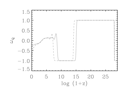
FIG. 6.: The dotted line represents the evolution of $\omega_{Q}$ for the potential $V(Q)=\Lambda^{4+\alpha}Q^{-\alpha}$ with $\alpha=11$ whereas the dashed line represents the evolution of the equation of state for the same value of $\alpha$ and for the SUGRA model presented in this article.

We see that the value of the equation of state today, for $\alpha=11$, is given by [15]:

$$\omega_{Q}\approx-0.82.$$ (77)

This is a remarkable property since in the context of usual tracking solutions it is not possible to obtain a number less than $\approx-0.7$ [11] whereas the observations seem to indicate that the value of the equation of state today is rather such that $-1\leq\omega_{Q}\leq-0.8$. We would like to note that this nice property is almost independent of $\alpha$. This is illustrated on the following figure where the relation $\omega_{Q}-\alpha$ is displayed

FIG. 7.: Equation of state $\omega_{Q}$ in function of $\alpha$ for the SUGRA model of quintessence proposed in this article.

The equation of state is almost independent of $\alpha$ because its value today is roughly speaking determined by the exponential term in the potential which is $\alpha$ independent. As a consequence, no fine tuning of $\alpha$ is required in order to obtain a reasonable value for $\omega_{Q}$.

The implications for structure formations of this model seem to be also very interesting and are currently under investigations [30].

More details on this model can be found in Ref. [15].

VI Conclusions

We have studied the quintessence scenario recently proposed in Ref. [13]. We have concentrated on models with an inverse power law potential and the diverse corrections induced by its embedding into High Energy Physics models. More particularly we have focused on the quantum corrections in the non-supersymmetric setting, the curvature and Kähler corrections in the supersymmetric case, and the effect of the non-renormalisable interaction suppressed by the Planck mass in the supergravity context. We have verified that quintessence is stable to the one-loop quantum corrections, preserving the existence of tracking solutions at small red-shift. We nevertheless argue that the solution to the fine-tuning problem requires to consider the quintessence models within the framework of particle physics beyond the standard model. Emphasizing the supersymmetric scenario, the most likely candidate to describe the physics beyond the weak scale, we generalize the usual inverse power law potential of the $SU(N_{\rm c})$ super-QCD case to more general supersymmetric gauge theories with Dynkin indices $\mu\leq\mu_{\rm adj}$. In supersymmetric models the quantum corrections to the superpotential vanish. However there are two types of potentially dangerous corrections. Firstly the smallness of the effective mass of the quintessence field implies that one must consider the small SUSY breaking induced by curvature effects. We show that these effects are not a threat to the quintessence scenario. Secondly we investigate the corrections to the Kähler potential and show that they play only a role at the beginning of the evolution, decoupling at a scale of the order of the gaugino condensation scale, and are strong enough to jeopardize the quintessence property. Far more relevant is the necessary inclusion of dangerous supergravity corrections due to the presence of Planck mass suppressed interactions which induce negative contributions to the potential at small red-shift. They destroy the quintessence property if the quintessence models are not treated within the realm of SUGRA.

This is what we do in the final section considering models where the expectation value of the superpotential vanishes altogether. This prevents the appearance of the negative contributions to the energy density. We give two explicit models where this scenario is at work. One is based on the heterotic string at weak coupling, the role of the quintessence field being played by a moduli. The run-away behaviour of the moduli is of the exponetial type limiting the possible contribution to the energy density to $\Omega_{Q}=0.15$ per moduli. In usual orbifold compactification this can amount to a $\Omega_{Q}=0.45$ contribution. Finally we present an existence proof of an inverse power law potential in SUGRA by constructing a model based on a particular Kähler potential. This model is particularly promising as it provides a scenario for which the value of $\omega_{Q}$ is $-0.82$ for $\Omega_{\rm m}=0.3$. This is within one sigma of the recent experimental analyses [9].

Let us emphasize that the models of quintessence within the framework of SUSY or SUGRA suffer from a problem raised in [12] concerning the necessary breaking of supersymmetry. Indeed there are two aspects to this problem, both linked to the types of corrections considered here. Let us first deal with the SUSY case. As advocated in [12] the present of a non-zero $F=M_{\rm S}^{2}$ term of the order $10^{10}\mbox{GeV}$ leads to an intolerably large value of the cosmological constant. This necessitates to invoke the prejudice already used in our paper that one does not know the mechanism which would force the cosmological constant to vanish. Quintessence scenarios do not aim at solving the quantum cosmological constant problem, see the conclusion of Ref. [18]. Another difficulty springs from the possible non-flatness of the Kähler potential and a coupling between the quintessence field $Q$ and the field responsible for the supersymmetry breaking leading to a term given by:

$${\rm\delta}V(Q)=k(Q)M_{\rm S}^{4},$$ (78)

where the series expansion of $k$ is a power series suppressed by the Planck scale. It gives a large contribution to the mass of $Q$ and the cosmological constant.

Of course one should repeat the arguments within the SUGRA context. At tree level one can always fine-tune the minimum of the potential to be zero. The power law expansion of the potential might just give a correction to the quintessence behaviour which would only modify the end of the evolution of $Q$ while preserving quintessence. In the explicit model of section V.C, the SUSY breaking is induced by the $F$ terms of the dilaton and the moduli. The dilaton does not couple directly to the quintessence field Q in the Kähler potential because of the anomalous $U(1)_{\rm X}$ symmetry. This implies that our model is not affected by a dilatonic SUSY breaking. Assuming the existence of a modular symmetry, we find that the effect of the SUSY breaking by the moduli is to induce terms like $F^{2}/Q^{2p}$ in the scalar potential. More studies are required to evaluate the effect of this term, in particular its order of magnitude. However, the fact that this term is proportional to the inverse of the quintessence field suggests that it will cause no problems. This question will be adressed elsewhere [31].

In conclusion we would like to emphasize the explicit construction of particle physics models leading to the quintessence property is still to be further developped. It seems to us clear that the indications given in this paper show that the building of SUGRA models should turn out to be very fruitful.

VII Appendix I: The effective Action in Curved Space

In the following we shall consider the case of curved spacetimes $R\neq 0$. Let us consider the following Lagrangian

$$S = -\int{\rm d}^{4}x\sqrt{-g}\biggr{(}{\rm\partial}_{\mu}\varphi{\rm\partial}^{\mu}\varphi^{*}+i\bar{\psi}\bar{\Sigma}^{\mu}{\rm D}_{\mu}\psi$$ (79)

$$+ \frac{m(\varphi)}{2}\psi\psi+\frac{\bar{m}(\varphi)}{2}\bar{\psi}\bar{\psi}+V(\varphi)\biggr{)},$$ (80)

where, for convenience, we have not written the spinorial indices. The mass and the potential are related to the superpotential $W$ as

$$m(\varphi)=\frac{{\rm\partial}^{2}W}{{\rm\partial}\varphi^{2}},\quad V(\varphi)=\biggl{|}\frac{{\rm\partial}W}{{\rm\partial}\varphi}\biggr{|}^{2}.$$ (81)

This is the usual globally supersymmetric Lagrangian coupled to gravity. As supersymmetry is not preserved by the background curved space the Lagrangian receives quantum corrections. The effective potential is renormalised due to the background geometry. Let us calculate this potential at the one loop level.

It is technically necessary to perform a Wick rotation to obtain a Euclidean field theory on a curved Riemannian manifold. This is globally feasible if one chooses the curved spacetime manifold to be a globally hyperbolic manifold with a Lorentzian signature. This implies that the time coordinate is globally defined allowing us to perform the appropriate rotation $t\to it$. In order to have a good control on the Feynman path integral it is convenient to expand the bosonic field $\varphi$ around the classical solution $\varphi_{\rm c}$ of the Klein-Gordon equation $-\Delta\varphi_{\rm c}+({\rm\partial}V/{\rm\partial}\varphi_{\rm c}^{*})=0$ where $\Delta$ is the curved Laplacian on the Riemannian manifold. Let us denote $\varphi=\varphi_{\rm c}+\tilde{\varphi}$ where $\tilde{\varphi}$ is a full-fledged quantum field. The effective potential does not involve derivatives of $\varphi_{\rm c}$, we will only retain non-derivative terms in the expansion of the effective action

$$e^{-S_{\rm eff}(\varphi_{\rm c})}=\int{\cal D}\tilde{\varphi}{\cal D}\psi{\cal D}\bar{\psi}e^{-S},$$ (82)

where $S_{\rm eff}$ is defined by the equation

$$S_{\rm eff}\equiv\int{\rm d}^{4}x\sqrt{g}V_{\rm eff}(\varphi_{\rm c}).$$ (83)

The effective potential is the sum of the classical part corrected by a quantum contribution

$$V_{\rm eff}(\varphi_{\rm c})=V(\varphi_{\rm c})+{\rm\delta}V(\varphi_{\rm c}).$$ (84)

The correction term is due to the integration over the Weyl fermions and the bosonic fields. To leading order the effective action is

$$S_{\rm eff}(\varphi_{\rm c})=\mbox{tr}\ln(\Delta+|m|^{2})-\frac{1}{4}\mbox{tr}\ln(\Delta_{\rm F}),$$ (85)

where $\Delta_{\rm F}$ is the operator $\Delta_{\rm F}={\rm D}_{\rm F}^{\dagger}{\rm D}_{\rm F}$ and

$${\rm D}_{\rm F}\equiv\left(\begin{array}[]{cc}i{\rm D}&\bar{m}\\ m&i\bar{\rm D}\\ \end{array}\right),$$ (86)

where ${\rm D}$ and $\bar{\rm D}$ are the Dirac operators acting on Weyl fermions of both chiralities. The previous expression can be computed using the $\zeta$ function regularisation where the determinant of an operator is $\det A=\exp[-\zeta_{\rm A}^{\prime}(0)]$ and the $\zeta$ function is $\zeta(s)=\sum_{n}1/\lambda_{n}^{s}$ as a function of the eigenvalues $\lambda_{n}$. The $\zeta_{\rm A}$ function is related to the heat kernel solution of

$$AG(x,x^{\prime},\sigma)=-\frac{\rm\partial}{{\rm\partial}\sigma}G(x,x^{\prime},\sigma),$$ (87)

with the boundary condition $G(x,x^{\prime},0)=\delta(x-x^{\prime})$ via the Mellin transform

$$\zeta_{\rm A}(s)=\frac{\mu^{2s}}{\Gamma(s)}\int_{0}^{\infty}{\rm d}\sigma\sigma^{s-1}\int{\rm d}^{4}x\sqrt{g}G(x,x,\sigma).$$ (88)

The scale $\mu$ is a renormalisation scale. The determinant of the operator $A$ is essentially given by the asymptotic expansion of the heat kernel

$$G(x,x,\sigma)\approx\frac{1}{(4\pi\sigma)^{2}}\biggl{(}1-\tau_{1}\sigma+O(\sigma^{2})\biggr{)},$$ (89)

leading to

$$\det A=\exp\biggl{(}\int{\rm d}^{4}x\sqrt{g}\frac{\tau_{1}^{2}}{32\pi^{2}}(\ln\frac{\tau_{1}}{\mu^{2}}-\frac{3}{2})\biggr{)}.$$ (90)

The asymptotic expansion of the Heat kernel of the operator $-\Delta+|m|^{2}$ gives $\tau_{1}=-R/6+|m|^{2}$ and for the Dirac operator it yields $\tau_{1}^{\rm F}=|m|^{2}+R/12$ where $R$ is the scalar curvature. The one loop effective potential is then

$${\rm\delta}V_{\rm eff}(Q,\eta) = \frac{1}{32\pi^{2}}\biggl{\{}\biggl{[}|m|^{2}-\frac{R}{6}\biggr{]}^{2}\biggl{[}\ln\biggl{(}\frac{|m|^{2}-R/6}{\mu^{2}}\biggr{)}-\frac{3}{2}\biggr{]}$$ (91)

$$- \biggl{[}|m|^{2}+\frac{R}{12}\biggr{]}^{2}\biggl{[}\ln\biggl{(}\frac{|m|^{2}+R/12}{\mu^{2}}\biggr{)}-\frac{3}{2}\biggr{]}\biggr{\}}.$$ (92)

Notice that the one loop correction vanishes if the curvature is zero.

VIII Appendix II: Supergravity Vacua

In this appendix we shall be interested in finding whether a given FLRW space time preserves supersymmetry. The FLRW background does not break supersymmetry in an explicit manner when the gravitino $\psi_{\mu}=0$ is invariant under supersymmetry transformations. We have assumed that the quintessence field $Q$ is only coupled to other field via the gravitational interactions. In a hidden sector the supergravity can be broken with a non-vanishing mass $m_{3/2}$ leading to the condition

$${\rm D}_{\mu}\epsilon+\frac{i}{2}m_{3/2}\sigma_{\mu}\bar{\epsilon}=0,$$ (93)

where $\epsilon$ is a Weyl spinor representing the supersymmetry variation. Computing the commutator $[{\rm D}_{\mu},{\rm D}_{\nu}]$ and using $R_{\mu\nu\rho\sigma}=(R/2)(\eta_{\mu\rho}\eta_{\nu\sigma}-\eta_{\nu\rho}\eta_{\mu\sigma})$, we find that the supersymmetry is generically broken apart from two cases. If the gravitino mass vanishes, the supersymmetry is fully preserved by FLRW spaces with vanishing curvature. When the gravitino mass is not zero the supersymmetry is not broken if the FLRW space is the anti-Desitter manifold with curvature $R=-m_{3/2}^{2}$.

REFERENCES

- [1] A. G. Riess et al., Astrophys. J. 116, 1009 (1998); P. M. Garnavich et al., Astrophys. J. 509, L74 (1998); S. Perlmutter et al., Astrophys. J. 516, (1999).
- [2] M. Tegmark, Astrophys.J. 514, L69 (1999).
- [3] C. B. Netterfield et al., Astrophys. J. 474, 47 (1997); E. Wollack et al., Astrophys. J. 476, 440 (1997);
- [4] K. Coble et al., astro-ph/9902195.
- [5] E. Torbet et al., astro-ph/9905100.
- [6] I. Zehavi and A. Dekel, astro-ph/9904221.
- [7] L. Wang, R. R. Caldwell, J. P. Ostriker and P. J. Steinhardt, astro-ph/9901388.
- [8] S. Perlmutter, M. S. Turner and M. White, astro-ph/9901052.
- [9] G. Efstathiou, astro-ph/9904356.
- [10] S. Coleman, Nucl. Phys. B 310, 643 (1988);
- [11] R. R. Caldwell, R. Dave and P. J. Steinhardt, Phys. Rev. Lett. 80, 1582 (1998);
- [12] C. Kolda and D. H. Lyth, hep-ph/9811375.
- [13] I. Zlatev, L. Wang and P. J. Steinhardt, astro-ph/9807002; P. J. Steinhardt, L. Wang and I. Zlatev, astro-ph/9812313;
- [14] P. Binétruy, hep-ph/9810553.
- [15] P. Brax and J. Martin, astro-ph/9905040.
- [16] K. Choi, hep-ph/9902292.
- [17] A. Masiero, M. Pietroni and F. Rosati, hep-ph/9905346.
- [18] P. J. E Peebles and B. Ratra, Phys. Rev. D 37, 3406 (1988).
- [19] S. Coleman and E. Weinberg, Phys. Rev. D 7, 1888 (1973).
- [20] S. Weinberg, Phys. Rev. D 7, 2887 (1973).
- [21] J. Iliopoulos, C. Itzykson and A. Martin, Rev. Mod. Phys.D 47, 165 (1975).
- [22] C. Csaki, M. Schmaltz and W. Skiba, Phys. Rev. D 55, 7840 (1997).
- [23] P. Brax, C. Grojean and C. A. Savoy, hep-ph/9808345.
- [24] L. P. Grishchuk and Y. V. Sidorov, Phys. Rev. D. 42, 3413 (1990).
- [25] J. Wess and J. Bagger, Supersymmetry and Supergravity, Princeton University Press.
- [26] L. Parker, Phys. Rev. D 3, 346 (1971).
- [27] M. Dine, N. Seiberg and E. Witten, Nucl. Phys. B 289, 589 (1988).
- [28] L. E. Ibanez and D. Lust, Nucl. Phys. B 382, 305 (1992).
- [29] P. G. Ferreira and M. Joyce, Phys. Rev. D 58, 023503-1 (1998); P. G. Ferreira and M. Joyce, Phys. Rev. Lett. 79, 4740 (1997); C. Wetterich, Nucl. Phys. B 302, 668 (1988).
- [30] P. Brax, J. Martin and A. Riazuelo, in preparation.
- [31] P. Brax, J. Martin, in preparation.