Fluctuations of Gravitational Wave Noise from Unresolved Extragalactic Sources

Abstract

Angular fluctuations of stochastic gravitational wave backgrounds (GWB) produced by extragalactic astrophysical sources are calculated. The angular properties of such backgrounds are determined by the large scale structure of Universe (galaxy clustering). The evolution of star formation rate with redshift is taken into account. Fluctuations of the metric strain amplitude associated with such noises at angular scales of about one degree are found to be of order 5-20% slowly growing toward smaller angular scales. This feature can be potentially used to separate astrophysical GWB from cosmological ones in future experiments.

1 Introduction

With the advent of detectors of gravitational waves (GW), which are currently under construction, a totally new possibility to study different astronomical objects opens up (Thorne 1988). In addition to ”classic” sources of GW like merging compact binaries or rapidly rotating hot neutron stars etc., which will be studied at frequencies $\sim 10-1000$ Hz, there should exist a specific cosmological background (noise) covering a very wide frequency band from $\sim 10^{-18}$ to $10^{5}$ Hz. The cosmological background should bear imprints of the physical processes in the very early Universe (Grishchuk 1988, 1997 and references therein). The primordial GW background, which originates from vacuum fluctuations parametrically amplified by the very expansion of the Universe, has a power-law spectrum spanning a very wide frequency range (Starobinsky 1979, Rubakov et al. 1982, Grishchuk 1988, 1997). The prospects for its detection appear to be the most favorable at the low frequency band ($10^{-3}-10^{-1}$ Hz) which will be covered by LISA space interferometer (Larson et al. 1999).

At some frequencies, however, unresolved binary stars within our own Galaxy or beyond provide an important contribution in the LISA frequency band (Bender and Hils 1997, Postnov and Prokhorov 1998, Kosenko and Postnov 1998). As shown in these papers, the stochastic signal from unresolved merging white dwarf binaries dominates the LISA sensitivity curve up to $\sim 3\times 10^{-3}$ Hz. At higher frequencies extragalactic merging white dwarf binaries contribute at a level roughly 10 times smaller, which is below the planned LISA sensitivity at these frequencies. This fact allows search for detection of the primordial GW backgrounds by LISA (Grishchuk 1997).

However, some inherent uncertainties (e.g. in the galactic rate of binary white dwarf mergings) are present in the calculations so the astrophysical backgrounds can turn out to be higher than expected. Since astrophysical GW backgrounds are considered as an additional noise contributing to the intrinsic noise of the detector, as much as possible of their properties at all frequencies should be known in advance.

What are specific features of astrophysical GW backgrounds? Clearly, those related to the galactic sources should follow the distribution of stars inside the Milky Way (Hils et al. 1989, Lipunov et al. 1995). As all the detectors (ground-based or space-born) should rotate with respect to the galactic plane, the signal modulation has been used as an advantage to detect them (Giazotto et al. 1997, Giampieri and Polnarev 1997). As for the backgrounds of extragalactic origin, only amplitudes at different frequencies from various sources have been computed so far (Kosenko and Postnov 1998, Ferrari et al. 1999a,b).

The purpose of the present paper is to study angular properties of the GW noise produced by extragalactic astrophysical sources at the degree scales. As most of these source must reside in galaxies (only a tiny fraction of binaries or GW-emitting neutron stars is expected to be in the intergalactic space), the GW background should have distinctive angular correlation properties reflecting the large scale structure (LSS) of the Universe. This is exactly what we observe in electromagnetic radiation as fluctuations of, for example, IR background observed by COBE (Kashlinsky et al. 1999).

2 Imprint of the LSS in the astrophysical GWB

The angular fluctuations of intensity in any astrophysical GWB should correlate with those of the projected number of galaxies, so first we wish to remind the reader the well-developed technique which is used for studies of angular properties of galactic counts on the sky. There is a lot of specially dedicated literature on this subject (see e.g. Peebles 1980, 1993). Before to proceed further, let us make a simple estimate. Suppose we have sources (galaxies) randomly distributed in space. What is the rms fluctuation of the number of galaxies within a small solid angle $\delta\Omega=\pi\theta^{2}\ll 4\pi$? With the average space density of galaxies $n_{G}\simeq 0.01$ Mpc^-3 and neglecting cosmological effects for a while we would get

$$\frac{\delta N(\theta)}{N}=\frac{1}{\sqrt{N(\theta)}} \sim \frac{1}{\sqrt{n_{G}}}\frac{1}{\theta}\,\left(\frac{c}{H_{0}}\right)^{-3/2}$$

$$\sim 3\times 10^{-2}\left(\frac{\theta}{0.01}\right)^{-1}\,,$$

(here $H_{0}$ is the Hubble constant) while galactic counts demonstrate a much higher value $\delta N/N\sim 0.5$ for linear scales $l=30$ Mpc (i.e. $\theta\sim 0.01$ for the most distant galaxies) (Peebles 1993). So clearly we should take into account the correlation properties of galaxies and galactic clusters.

To account for the non-Poissonian properties of galactic distribution in space, the correlation functions are used. For Gaussian fluctuations only two-point correlation function $\xi(\@vec{r})$ or its Fourier transform (power spectrum) $P_{3}(\@vec{k})$ would be sufficient. Taking $P_{3}(k)$ as derived from LSS studies, we then can calculate the 2-dimensional correlation function $C(\theta)$ of the projected distribution of galaxies on the sky or, equivalently, the 2-dimensional power spectrum $P_{2}(q)$. This is the last quantity that we actually need since the rms fluctuation of the energy flux per unit logarithmic frequency interval in a given direction is directly related to $P_{2}(q)$ (Kashlinsky et al. 1999 and below).

2.1 Correlation functions and power spectrum

The brightness of a GW background can be characterized by the energy flux coming from a given direction within a solid angle $\Delta\Omega$ (Thorne 1988)

$$f\frac{dE(\mathbf{x})}{dtdSdfd\Omega}\Delta\Omega=\int\limits_{\Delta\Omega}fI_{f}d\Omega$$ (2)

where $\mathbf{x}$ is the two dimensional coordinate across the sky. The integration over all sky yields the familiar value $\Omega_{GW}\rho_{cr}c^{2}$, the energy density per unitary logarithmic frequency interval in units of the critical energy density to close the Universe, which characterizes the isotropic stochastic GWB. To study angular properties of the noise we shall consider the flux from given direction $F(\mathbf{x})\equiv fI_{f}$ itself. We shall assume some ideal GW detector with a beam-like sensitivity diagram, which is of course far from realistic ground-based LIGO-like or spaceborn LISA-like interferometers. However, in this paper we will not discuss the observability of GW backgrounds.

The fluctuation in the GW flux arrived at the detector from a given direction on the sky is $\delta F(\mathbf{x})=F(\mathbf{x})-\langle F\rangle$, where $\langle\ldots\rangle$ denotes ensemble averaging. The Fourier transform of the fluctuation is $\delta F(\mathbf{\theta})=1/(2\pi)^{2}\int\delta F_{q}\exp(-i\mathbf{q}\mathbf{\theta})d^{2}\mathbf{q}$.

The projected 2-dimensional correlation function represents the first non-trivial moment of the probability distribution function of $\delta F(\mathbf{x})$: $C(\mathbf{\theta})=\langle\delta F(\mathbf{x}+\mathbf{\theta})F(\mathbf{x})\rangle$. The two dimensional power spectrum is by definition $P_{2}(q)=\langle|\delta F_{q}|^{2}\rangle$. We shall assume the phases to be random and the distribution of the flux field to be Gaussian so that the power spectrum is just the Fourier transform of the correlation function:

$$C(\theta)=\frac{1}{2\pi}\int_{0}^{\infty}P_{2}(q)J_{0}(q\theta)qdq\,,$$ (3)

$$P_{2}(q)=\int_{0}^{\infty}C(\theta)J_{0}(q\theta)\theta d\theta\,.$$ (4)

Here $J_{0}$ is the zero-order cylindrical Bessel function.

The mean square fluctuation of the flux on the detector within a finite solid angle $\Delta\Omega$ subtended by the angle $\vartheta$ across the sky is zero-lag correlation signal

$$\langle(\delta F)^{2}\rangle_{\vartheta}=\frac{1}{2\pi}\int_{0}^{\infty}P_{2}(q)W(q\vartheta)qdq$$ (5)

where $W$ is the window function of the detector. For example, for a top-hat beam $\langle(\delta F)^{2}\rangle_{\vartheta}\sim(1/2\pi)q^{2}P_{2}(q)|_{q\sim\pi/2\vartheta}$ and the values of $1/q$ correspond to fluctuations of angular size $\sim\pi/q$.

The GWB flux and its angular properties measured in projection on the celestial sphere should reflect 3-dimensional structure of the Universe and the change of GW emission rate with redshift $z$. The LSS can be taken into account by the 3-dimensional correlation function $\xi(r)$ or its 3-dimensional power spectrum $P_{3}(k)$, which for isotropic case relates to $\xi(r)$ through the equation

$$\xi(r)=\frac{1}{2\pi^{2}}\int_{0}^{\infty}P_{3}(k)j_{0}(kr)k^{2}dk$$ (6)

(here $j_{0}$ is the zero-order spherical Bessel function).

The projected correlation function of cosmic GWB $C(\mathbf{\theta})$ is expressed through two-point correlation function of the galaxy distribution $\xi(r_{12})$ and the rate of GW emission $dF/dz$ via the Limber equation (Limber, 1953):

$$C(\mathbf{\theta})=\int\left(\frac{dF}{dz_{1}}\right)\left(\frac{dF}{dz_{2}}\right)\xi(r_{12},z)dz_{1}dz_{2}$$ (7)

Substituting this equation in the limit of small angles $\theta\ll 1$ for Friedman-Robertson-Walker metrics into Eq. (4) one gets (Kashlinsky et al. 1999)

$$P_{2}(q)=\int_{0}^{\infty}\left(\frac{dF}{dz}\right)^{2}\frac{P_{3}(\frac{q}{d_{A}(z)},z)}{d_{A}^{2}(z)c\frac{dt}{dz}}dz$$ (8)

where $d_{A}=d_{m}/(1+z)$ is the angular distance, $d_{m}$ is the metric distance. For degree angular scales of interest here the linear approximation of galactic clustering can be used $P_{3}(k,z)\simeq P_{3}(k,0)\times\Psi(z)$, where $\Psi(z)$ describes the evolution of the clustering. On linear scales $\Psi(z)=(1+z)^{-1}$ if $\Omega=1$ (Peebles, 1980).

In our analysis we use the 3D spectrum $P_{3}(k)$ as derived by Einasto et al. (1999) from a thorough analysis of different LSS studies. The mean spectrum of galaxies shows a power-law behavior at small and large $k$ with a maximum $\sim 10^{4}[h^{-3}\hbox{Mpc}^{3}]$ at $k\approx 5\times 10^{-2}\,h\,\hbox{Mpc}^{-1}$.

The analysis of this formula (Kashlinsky et al. (1999) and references therein) shows that the relative fluctuations of the flux are $\delta F_{rms}\sim\sqrt{H_{0}/ck^{2}P_{3}(k)}\sim 5\%-10\%$ and weakly dependent on the cosmological model at angular scales of order one degree. However, strong dependence on redshift of the flux rate requires more accurate calculations.

2.2 GWB flux

The GW energy emitted by the population of some sources in a galaxy at frequency $f$ per unit logarithmic frequency interval $d\ln f$ in the rest-frame of the galaxy can be calculated through the rate of GW-producing events ${\cal R}$ (e.g. the rate of binary WD mergings or supernova explosions) in the galaxy. Under the stationary conditions we have (Kosenko and Postnov 1998)

$$\frac{dE}{dtd\ln f}={\cal R}\frac{E(f)}{dt}\left(\frac{d\ln f}{dt}\right)^{-1}_{GW}$$ (9)

where $E(f)$ is the energy which is being carried away by gravitational waves from the typical source (e.g. for two point masses orbiting each other it is just the orbital binding energy). If $E(f)\propto f^{\alpha}$ and GW emission is the only dissipative mechanism

$$\frac{dE}{dtd\ln f}=\alpha{\cal R}E(f)$$ (10)

The comoving luminosity at proper frequency $f^{\prime}$ per unit logarithmic frequency interval produced by sources in galaxies at redshift $z$ from the redshift interval $dz$ from unit solid angle

$$\frac{d{\cal L}(f^{\prime},z)}{dz}=n(z)\frac{\delta V(z)}{dz}\frac{dE(f^{\prime})}{dtd\ln f^{\prime}}$$ (11)

where $n(z)$ is the space density of galaxies, $\delta V(z)$ is the proper volume element. We assume no new galaxies to create since their formation so that $n(z)=n_{G}(1+z)^{3}$ and $n_{G}=0.013(\Omega_{b}/0.005)h_{100}^{2}$ Mpc^-3 is the present-day density of galaxies normalized to the amount of baryons comprised in stars (in terms of the critical energy density $\rho_{cr}c^{2}$; $h_{100}\equiv H_{0}/100$(km/s/Mpc) is the Hubble constant). The strong star formation rate evolution is taken into account through the evolution of the event rate with redshift ${\cal R}(z)$ (Kosenko and Postnov 1998). We use the parametrization of Rowan-Robinson (1999) for the star formation rate history SFR$(z)$ as derived from optical, UV, and IR-observations, and normalized to unity at $z=0$. The rate of particular events is thus ${\cal R}(z)={\cal R}_{G}\int\limits_{z_{*}}^{0}\hbox{SFR}(z^{\prime})G(z-z^{\prime})dz^{\prime}$ where ${\cal R}_{G}$ is the present-day event rate per galaxy, $G(z-z^{\prime})$ is the redshift dependence of the rate after a $\delta$-function-like star formation burst. This is important especially for binary white dwarf coalescences because these are delayed typically by $\sim 10^{9}$ years since their formation. For events which relate to massive star evolution, like supernova explosions, we have $G(z-z^{\prime})\approx\delta(z-z^{\prime})$ and the change in the rate of events with redshift simply follows the star formation rate evolution ${\cal R}(z)={\cal R}_{G}\times\hbox{SFR}(z)$.

The proper volume element is (Peebles 1993)

$$\frac{\delta V(z)}{dz}=c\frac{dt}{dz}\frac{d_{m}(z)^{2}}{(1+z)^{2}}$$ (12)

with the metric distance $d_{m}$ and $dt/dz$ being the functions of the cosmological model (Carroll et al. 1992). In our calculations we use the standard flat universe without cosmological constant and a $\Lambda$-term dominated cosmological model with $\Omega_{\Lambda}=0.7$, $\Omega_{m}=0.3$.

Combining equations (10), (11), and (12) together we arrive at

$$\frac{d{\cal L}(f^{\prime},z)}{dz}=c\frac{dt}{dz}d_{m}^{2}(z)(1+z)n_{G}{\cal R}(z)E(f^{\prime})\alpha$$ (13)

so the contribution to the total GW flux from the redshift interval $dz$ from unit solid angle which is observed today by a detector with band-width $df$ centered at frequency $f=f^{\prime}/(1+z)$ is

$$\frac{dF(f)}{dz} \equiv \frac{dE(f)}{dt\;dS\;d\ln f\,dz}$$

$$= \left(\frac{d{\cal L}(f(1+z),z)}{dz}\right)\frac{1}{4\pi d_{L}^{2}}$$

$$= \alpha{\cal R}_{G}(z)n_{G}E(f)\frac{(1+z)^{\alpha-1}}{4\pi}\frac{cdt}{dz}$$

where we used the luminosity distance definition $d_{L}=d_{m}(1+z)$. Note that no additional factor $(1+z)$ accounting for the change of frequency interval appears in the numerator since we are working with unitary logarithmic frequency interval.

Now we are in the position to calculate relative fluctuations $\delta F/F$ of any GWB produced by astrophysical sources associated with galaxies within a given solid angle $\theta\ll 1$. From Eqs. (8) and (2.2) we derive

$$\frac{\delta F(q)}{F} = \Biggl{(}\int\limits_{0}^{z_{*}}\left(\frac{{\cal R}(z)}{{\cal R}_{G}}\right)^{2}(1+z)^{2\alpha-2}\Psi^{2}(z)\left(\frac{c\;dt}{dz}\right)\times$$

$$\hphantom{\Biggl{(}\int\limits_{0}^{z_{*}}}\times\left(\frac{q}{d_{A}(z)}\right)^{2}P_{3}\left(\frac{q}{d_{A}(z)}\right)dz\Biggr{)}^{1/2}\Big{/}$$

$$\Big{/} \int\limits_{0}^{z_{*}}\left(\frac{{\cal R}(z)}{{\cal R}_{G}}\right)(1+z)^{\alpha-1}\left(\frac{cdt}{dz}\right)dz$$

Here the redshift $z_{*}$ corresponds to the beginning of star formation in the Universe. In our calculations we assumed $z_{*}=10$ (in fact, the exact value is of minor importance since sources at small and moderate redshifts mostly contribute to the flux).

For stochastic GWB the flux per unit logarithmic frequency interval is related to the dimensionless strain amplitude $h$ as

$$h=\left(\frac{2G}{\pi c^{3}f^{2}}\right)^{1/2}F(f)^{1/2}$$ (16)

so at a given frequency fluctuations in the strain amplitude $\delta h/h=(1/2)(\delta F/F)$.

Note that the value of fluctuations depends on the specific source type only through the dependence of energy carried away by gravitational waves on frequency (index $\alpha$ for the power-law dependence) and the dimensionless change of event rate with redshift $\left(\frac{{\cal R}(z)}{{\cal R}_{G}}\right)$. The dependence on frequency can appear only through the change in spectral index $\alpha$ with frequency. To ensure that the spectral shape has no effect on the relative fluctuations, observations should be performed at a frequency which is sufficiently (by an order of magnitude) lower than the high-frequency cut-off of the comoving power-law spectrum of the background.

2.3 Specific examples

As specific examples we consider GWB produced by extragalacting merging white dwarfs and rapidly rotating hot neutron stars. In the first case the energy carried away by gravitational radiation is the orbital energy of binary white dwarfs whose evolution is driven by gravitation wave emission. In the LISA sensitivity frequency band $10^{-4}-10^{-1}$ Hz we have $E(f)\sim f^{2/3}$, $\alpha=2/3$. A white dwarf binary system reaches the orbital frequency of the pre-merging stage $10^{-2}$ Hz typically $\sim 10^{9}$ years after the formation, so the dependence of the rate of events on redshift goes smoother than star formation rate history SFR$(z)$ in the Universe. The isotropic stochastic GWB produced by extragalactic binary white dwarfs with account of the star formation rate evolution in the Universe was calculated by Kosenko & Postnov (1998). At the frequency $0.01$ Hz its level is $h_{wd}\sim 5\times 10^{-21}$.

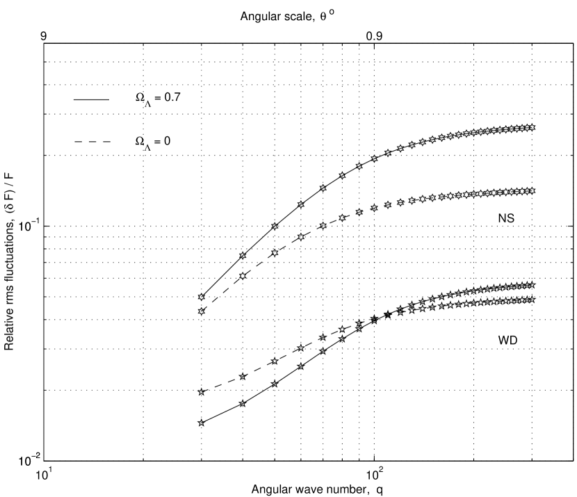
Figure 1: Relative rms fluctuation of the gravitational wave flux from unresolved extragalactic astrophysical sources at different angular scales $\theta=\pi/q$. Shown are fluctuations of the backgrounds produced by hot rapidly rotating neutron stars at frequency 100 Hz (upper curves) and by coalescing binary white dwarfs at frequency $10^{-2}$ Hz (lower curves). Calculations for flat FRW universes without cosmological constant ($\Omega_{L}=0$) and with $\Omega_{L}=0.7$.

For hot young neutron stars the emission of gravitational waves can be driven by r-mode instability (Lindblom et al. 1998, Owen et al. 1999). The energy carried away by gravitational waves is the rotational energy of the neutron star $E_{r}$ and $E_{r}(f)\sim f^{2}$ (i.e. $\alpha=2$) within the frequency band $\sim 120\,\hbox{Hz}<f<(2/3\pi)\Omega_{K}$, where $\Omega_{K}$ is the Kepler frequency at which mass shedding at the stellar equator makes the star unstable. The isotropic stochastic GWB produced by hot NS was studied by Ferrari et al. (1999b). Hot neutron stars are formed in the core collapse supernova explosion events in the end of evolution of massive stars, so no deviation from star formation dependence on redshift for their rate is expected. The isotropic background level at 100 Hz was estimated to be $h\sim 3\times 10^{-25}$.

The relative fluctuations of these backgrounds at angular scales $\theta=\pi/q$ are shown in Fig. 1 as a function of wave numbers $q$. It is seen that at $\theta\mathrel{\hbox to0.0pt{\lower 3.0pt\hbox{$\mathchar 536\relax$}\hss}\raise 2.0pt\hbox{$\mathchar 316\relax$}}1$ degree ($q\mathrel{\hbox to0.0pt{\lower 3.0pt\hbox{$\mathchar 536\relax$}\hss}\raise 2.0pt\hbox{$\mathchar 318\relax$}}100$), where the (quasi)linear regime of the galaxy clustering evolution with redshift is expected so that we can use $\Psi(z)=(1+z)^{-1}$, the fluctuations amount to 5% for coalescing white dwarfs and 10-20% for hot neutron stars. At larger scales (smaller $q$) the relative fluctuations slowly decrease. The calculations were performed for two cosmological models: a flat FRW universe with zero cosmological constant and with $\Omega_{\Lambda}=0.7$. In the case of hot neutron stars the level of fluctuations increases in the $\Lambda$-dominated Universe at all scales considered, while in the case of coalescing white dwarfs the curves for two cosmological models intersect at $q\sim 110$ (angular scales $\theta\sim 1.5$ degrees).

Note that at smaller angular scales (larger $q$) the non-linear evolution of LSS should be taken into account, so the present calculations cannot be applied.

3 Conclusion

We have calculated the expected level of angular fluctuations of cosmic stochastic gravitational wave backgrounds produced by populations of astrophysical sources associated with galaxies. The dependence of the source formation rate on redshift is taken into account using global star formation history in the Universe. The relative rms fluctuations of the GW flux does not depend on the specific source formation rate per galaxy, only on its evolution with redshift. The level of relative flux fluctuations at angular scales $\theta\mathrel{\hbox to0.0pt{\lower 3.0pt\hbox{$\mathchar 536\relax$}\hss}\raise 2.0pt\hbox{$\mathchar 316\relax$}}1$ degree is found to be $\sim 5\%$ for coalescing white dwarfs with insignificant dependence on the cosmological model assumed, and $10-25\%$ for hot neutron stars, with stronger fluctuations for flat cosmological constant dominated Universe. Angular dependence of these fluctuations is a distinctive feature of such GW backgrounds and can be used to discriminate between astrophysical and relic cosmological stochastic noises in future experiments.

We thank Prof. A.V.Zasov for useful notes. The work was partially supported by Russian Fund for Basic Research through Grant No 98-02-16801, the grant University of Russia 5559, and Royal Society Grant RCPX219.

References

- (1) Bender, P.L., Hils, D., 1997, Class. Quantum Grav., 14, 1439
- (2) Carroll, S.M., Press, W.H., Turner, E.L. 1992, Ann. Rev. Astron. Astrophys., 30, 499
- (3) Einasto, J. et al. 1999, ApJ, 519, 469
- (4) Ferrari V., Matarrese S., Schneider R. 1999a, MNRAS, 303, 247
- (5) Ferrari V., Matarrese S., Schneider R. 1999b, MNRAS, 303, 258
- (6) Giampieri, G., Polnarev, A.G., 1997, MNRAS, 291, 149
- (7) Giazotto A., Bonazzola S., Gourgoulhon E., 1997, Phys. Rev., D55, 2014
- (8) Grishchuk L.P. 1988, Uspekhi Fiz. Nauk 156, 297; English translation in Astrophysics and Space Physics Reviews, 7, 269 (1989).
- (9) Grishchuk, L.P. 1997, Class. Quantum Grav., 14, 1445.
- (10) Hils, D.L., Bender, P., Webbink, R.F. 1990, ApJ, 360, 75
- (11) Kashlinsky A., Mather J.C., Odenwald S. 1999, ApJ in press, astro-ph/9908304
- (12) Kosenko D.I., Postnov K.A. 1998, AA 336, 786
- (13) Larson S.L., Hiscock W.A., Hellings R.W. 1999, astro-ph/9909080
- (14) Limber D.N., 1953, ApJ, 117, 134
- (15) Lindblom L., Owen B.J., Morsink S.M. 1998, Phys. Rev. Lett. 80, 4843
- (16) Lipunov V.M., Nazin S.N., Panchenko I.E., Postnov K.A., Prokhorov M.E. 1995, AA, 298, 677
- (17) Madau, P., Ferguson, H.C., Dickinson, M. et al. 1996, MNRAS, 283, 1388
- (18) Madau, P., Pozzetti, L., Dickinson, M. 1997, ApJ, 498, 106
- (19) Owen B.J. et al. 1999, Phys. Rev., D5814834
- (20) Peebles P.J.E. 1980, The Large-Scale Structure of the Universe Princeton Univ. Press, Princeton, NJ
- (21) Peebles P.J.E. 1993, Principles of Physical Cosmology, Princeton Univ. Press, Princeton, NJ
- (22) Postnov, K.A., Prokhorov, M.E. 1998, ApJ, 494, 674
- (23) Rowan-Robinson M. 1999, astro-ph/9906308
- (24) Rubakov V.A., Sazhin M.V., Veryaskin A.V., 1982, Phys. Lett., B115, 189
- (25) Starobinsky A.A., 1979, JETP Lett., 30, 719
- (26) Thorne K.S., 1987, in 300 Years of Gravitation, Eds. S.W.Hawking and W.Israel (Cambridge University Press, Cambridge, England)