Effects of inflationary bubbles on the polarization and temperature anisotropies of the cosmic microwave background

Abstract

We predict the imprint of linear bubbly perturbations on the polarization and temperature anisotropies of the cosmic microwave background (CMB).

We analytically model a bubbly density perturbation at the beginning of the radiation dominated era and we apply the linear theory of cosmological perturbations to compute its time evolution. At decoupling, it uniquely signs the CMB polarization and temperature anisotropy sky. As predicted by recent general work regarding spatially limited cosmological seeds, during evolution the perturbation propagates beyond the size of the bubble and reaches the CMB sound horizon at the time considered. Therefore, its signal appears as a series of concentric rings, each characterized by its own amplitude and sign, on the scale of the sound horizon at decoupling ($\leq 1^{o}$ on the sky). Polarization and temperature rings are strictly correlated; photons coming from the center of the bubble are not polarized, because of the spherical symmetry of the present problem. As expected for linear perturbations with size $L$ and density contrast $\delta$ at decoupling, $\delta T/T$ is roughly $\delta(L/H^{-1})^{2}$; the polarization is about $10\%$ of the temperature anisotropy.

We predict the impact of a distribution of bubbles on the CMB polarization and temperature power spectra. Considering models containing both CDM Gaussian and bubbly non-Gaussian fluctuations, we simulate and analyze $10^{o}\times 10^{o}$ sky patches with angular resolution of about $3.5^{{}^{\prime}}$. The CMB power associated with the bubbles is entirely on sub-degree angular scales ($200\leq l\leq 1000$), that will be explored by the forthcoming high resolution CMB experiments with the percent precision. Depending on the parameters of the bubbly distribution we find extra-power with respect to the ordinary CDM Gaussian fluctuations; we infer simple analytical scalings of the power induced by bubbly perturbations and we constrain our parameters with the existing data.

1 Introduction

World wide theoretical and experimental efforts to understand what we could learn from the Cosmic Microwave Background (CMB) are presently in progress. Anisotropies in the CMB should contain precious details about high energy physics processes occurred in the early universe, still hidden to our knowledge. Reasonably, these processes left traces that have been stretched out to large and observable scales by an early era of accelerate expansion, called inflation; at decoupling between matter and radiation, these traces imprinted anisotropies in the CMB, thus being possibly detected and recognized.

Recently, the treatment of the linear CMB inhomogeneities has been put in a complete and organic form [Hu et al. 1997]. At the same time, many experiments are at work to explore the CMB anisotropies toward smaller and smaller angular scales [see Lasenby et al. 1998, De Bernardis et al. 1998 and references therein]; they shall culminate with the Planck mission of the next decade, that will provide the whole sky anisotropy map down to a minimum $\delta T/T\simeq 10^{-6}$ and an angular resolution of about $10^{{}^{\prime}}$ [see the Planck Surveyor and Microwave Anisotropy Probe home pages].

According to the simplest inflationary phenomenology, at very high energy in the early universe ($T\simeq 10^{-5}$ Planck masses), a scalar field slowly rolls toward the minimum of its potential, giving the non-zero vacuum energy responsible for the expansion itself. The quantum fluctuations generated during this phase are stretched out by the inflationary expansion itself to large scales and become the perturbations we observe today in the matter power spectrum [see Mukhanov, Feldman & Branderberger 1992 for an extensive treatment]. However, this is not the only known inflationary mechanism. Many fundamental fields may act on stage and the effective potential may have several minima separated by potential barriers. If this is the case quantum tunneling occurs, and the nucleated bubbles are stretched out to large scales just like the ordinary quantum fluctuations. At reheating the energy stored in the bubble shell is converted into matter and radiation and a bubbly trace is left in the density distribution. Tunneling processes are predicted in the context of first order inflation [see Kolb 1991 and references therein]; the possibility that bubbles have left traces in the large scale matter distribution was considered in the last decade [see Amendola et al. 1996 and references therein], in connection with the increasing observational evidence of large voids in the galaxy distribution [El-Ad, Piran & da Costa, 1997].

The aim of this work is to accurately predict the CMB polarization and temperature anisotropies from bubbly density perturbations existing at decoupling, relics of the inflationary tunneling phenomena. In an early work [Baccigalupi et al. 1997] we considered anisotropies from non-linear bubbles mainly for what concerns metric induced perturbations. Then, more recently [Baccigalupi 1998] we used an approximated method to compute the temperature anisotropies $\delta T/T$ from isolated inflationary bubbles in linear regime; we found that, just like a pebble in a pond, the bubbly perturbation generates anisotropy waves, traveling outward with the CMB sound velocity and reaching the scale of the sound horizon at the time we are examining it. Therefore, the image of an inflationary bubble at decoupling is a series of concentric isothermal rings of different color (sign of $\delta T/T$) on the scale of the sound horizon at decoupling ($\leq 1^{o}$ in the sky). In a separate work [Amendola, Baccigalupi & Occhionero 1998] we explored the impact of a distribution of bubbles on the CMB temperature angular power spectrum, finding for a wide set of statistical parameters extra power on sub-degree angular scales.

Here we compute the CMB polarization anisotropies induced by inflationary bubbles, and we generalize previous results on the temperature in the context of the full linear theory of cosmological perturbations [Ma & Bertschinger 1995]. We model the remnant of an inflationary bubble as a linear bubbly perturbation in the density distribution at the beginning of the radiation dominated era. Each Fourier mode is analytically calculated and numerically evolved following the linearized Einstein and Boltzmann equations. We use these results to study the signal from a single bubble. Regarding the size and density contrast of the bubbles, they are ultimately determined by the epoch of nucleation during inflation and by the properties of the tunneling barrier, so that these parameters depend on the details of the inflationary potential [see Amendola et al. 1996 and references therein]; as in previous works [Baccigalupi 1998, Amendola, Baccigalupi & Occhionero 1998] here we choose the bubble properties corresponding to the large voids observed in the galaxy distribution [El-Ad, Piran & da Costa, 1997], that have deep cavities $\delta\rho/\rho\simeq 1$ and comoving radii of about $20\div 40h^{-1}$ Mpc; if they are of primordial origin, the evolution from decoupling to the present implies an overcomoving growth by a factor of 2, and the density contrast increases approximatively linearly with the scale factor [Occhionero et al. 1998]: thus, the voids corresponding to the present ones should have at decoupling a comoving radius $R=10\div 20h^{-1}$ Mpc and density contrast $\delta=10^{-3}\div 10^{-2}$, values that we adopt in this work.

Starting from the signal from isolated bubbles, we predict the effect of a distribution of bubbles on the CMB temperature and polarization power spectra; as expected in scenarios admitting a bubble nucleating era during the inflationary slow roll [see Amendola et al. 1996 and references therein], we consider models containing a population of bubbles together with ordinary CDM Gaussian perturbations; in this context we simulate CMB sky maps and we compute the anisotropy angular power spectrum for various bubbly distribution parameters. As a general useful comment here, we wish to emphasize that both in the cases of a single bubble and a distribution of them, the signals treated here are definitely different from Gaussian perturbations. Gaussianity means that the fluctuations exhibit a completely disordered spatial distribution; only in this case the CMB angular power spectra tell us everything about the signal. On the contrary a bubbly perturbation is an ordered structure: it really possesses a spherical symmetry. Technically speaking, its signal is non-Gaussian; therefore, even if the CMB power spectrum is a powerful tool to investigate also non-Gaussian models, it does not fix completely the underlying fluctuations, and other methods should be adopted to investigate which type of non-Gaussian ordered pattern is present on the observed map. The general treatment of CMB anisotropies from cosmological structures having spatial finite extension and symmetries has been recently treated in detail [Baccigalupi 1999]; we apply the general treatment developed in that work to the present case.

The paper is organized as follows: in section II we recall the relevant equations for our purposes and we expose the computational details; in section III we evolve the bubbly perturbation to study the corresponding CMB perturbation at different times and to predict the effect on the CMB polarization and temperature anisotropies from isolated bubbles; in section IV we consider several distributions of bubbles and we predict their imprint on the CMB angular power spectra, also giving simple scalings in terms of the distribution parameters; finally, section V contains the conclusions.

2 The equations system

The evolution equations for fluid and CMB quantities may be obtained by the Boltzmann and linearized Einstein equations [Ma & Bertschinger 1995, Hu et al. 1997]. A standard CDM flat background is assumed, including cold dark matter (_c), baryons (_b), photons (_γ) and three families of massless neutrinos (_ν). The background flat Friedmann Robertson Walker (FRW) metric is

$$ds^{2}=a(\eta)^{2}\left(-d\eta^{2}+dr^{2}+r^{2}d\Omega^{2}\right)\ ,$$ (1)

where $\eta(t)=\int_{0}^{t}d\tau/a(\tau)$ is the conformal time. The background evolution is driven by the Einstein equation

$${\dot{a}^{2}\over a^{2}}={8\pi G\over 3}a^{2}\sum_{x}\rho_{x}\ ,$$ (2)

where the index $x$ runs over all the fluid species; the background parameters are $\Omega_{0}=1,h=.5,\Omega_{b}=0.05,\Omega_{CDM}=1-\Omega_{b}$. The perturbed metric tensor is

$$g_{\mu\nu}=a(\eta)^{2}(\gamma_{\mu\nu}+h_{\mu\nu})\ ,$$ (3)

where $a(\eta)^{2}\gamma_{\mu\nu}$ represents the background. Since $h_{\mu\nu}\ll\gamma_{\mu\nu}$, a gauge freedom reduces the number of physically significant quantities in the perturbation metric tensor; in this work we adopt the generalized Newtonian gauge in which the two scalar perturbed metric component are $\Psi=h_{00}/2$ and $2\Phi=h_{11}=h_{22}=h_{33}$ [Ma & Bertschinger 1995]; concerning the fluid, $\delta_{x}$ indicates the density contrast $\delta\rho/\rho$ for the species $x$ and $v_{x}$ its peculiar velocity in the background metric. Unless otherwise specified, all the equations for the perturbed quantities in the remaining part of this section are written in Fourier space, and the wavenumber argument is omitted.

The equations for the matter species are:

$$\dot{\delta}_{c}=-kv_{c}-3k^{2}\dot{\Phi}\ ,\ \dot{v}_{c}=-{\dot{a}\over a}v_{c}+k\Psi\ ,$$ (4)

$$\dot{\delta}_{b}=-kv_{b}-3k^{2}\dot{\Phi}\ ,\ \dot{v}_{b}=-{\dot{a}\over a}v_{b}+k\Psi+{4\rho_{\gamma}\over 3\rho_{b}}an_{e}\sigma_{T}(v_{\gamma}-v_{b})\ ,$$ (5)

where $\dot{\tau}=ax_{e}n_{e}\sigma_{T}$ is the differential optical depth; $\sigma_{T}$ is the Thomson scattering cross section, $n_{e}$ is the electron number density and $x_{e}$ the ionization fraction [see Hu & Sugiyama 1995 for useful fitting formulas].

Now we give the expressions for the CMB temperature and polarization perturbations in the context of a spherical perturbation field; these formulas have been recently developed [Baccigalupi 1999]. As customary, we indicate the temperature perturbation $\delta T/T$ with $\Theta$ and the linear polarization amplitude with the Stokes parameters $Q$, $U$.

Temperature perturbation carried by CMB photons scattered on an arbitrary direction $\hat{n}$ at a spacetime position $(\eta,\vec{r})$ around a spherical structure is given by

$$\Theta=\sum_{l}P_{l}(\hat{n}\cdot\hat{r})\int{k^{2}dk\over 2\pi^{2}}\Theta_{l}(\eta,k)j_{l}(kr)\ ,$$ (6)

where $P_{l}$ and $j_{l}$ are respectively Legendre polynomials and fractional order Bessel functions. All the specifications regarding the perturbation source are encoded in the $\Theta_{l}$ coefficients, which obey evolution equations that we shall write in a moment. Concerning the polarization, we have to specify the frame axes describing the polarization tensor on the plane perpendicular to $\hat{n}$. We choose them parallel and perpendicular to the plane formed by $\hat{n}$ and $\hat{r}$; with this choice, the polarization tensor is described only by $Q$ [Baccigalupi 1999] in the following way:

$$Q=\sum_{l\geq 2}\sqrt{(l-2)!\over(l+2)!}P_{l}^{2}(\hat{n}\cdot\hat{r})\int{k^{2}dk\over 2\pi^{2}}E_{l}(\eta,k)j_{l}(kr)\ .$$ (7)

$P_{l}^{2}$ are second order Legendre polynomials; this is a significant difference from (6): correctly, they make photons moving radially not polarized ($P_{l}^{2}(\pm 1)=0$). Again all the characteristics of the perturbation source are contained in the $E_{l}$ quantities. Now we give the evolution equations for the $E_{l}$ and $\Theta_{l}$ coefficients. They are the amplitudes of polarization and temperature CMB perturbations expanded in scalar and tensor spherical harmonics [Hu et al. 1997], and obey the following equations:

$$\dot{\Theta}_{0}=-{k\over 3}\Theta_{1}-\dot{\Phi}\ ,$$ (8)

$$\dot{\Theta}_{1}=k\Theta_{0}-{2\over 5}k\Theta_{2}+\dot{\tau}(v_{b}-\Theta_{1})+k\Psi\ ,$$ (9)

$$\dot{\Theta}_{2}={2\over 3}k\Theta_{1}-{3\over 7}k\Theta_{3}-\dot{\tau}\left({9\over 10}\Theta_{2}-{\sqrt{6}\over 10}E_{2}\right)\ ,$$ (10)

$$\dot{E}_{2}=-{\sqrt{5}\over 7}kE_{3}-\dot{\tau}\left({1\over 10}\Theta_{2}+{2\over 5}E_{2}\right)\ ,$$ (11)

and for $l\geq 3$

$$\dot{\Theta}_{l}=k\left[{l\over 2l-1}\Theta_{l-1}-{l+1\over 2l+3}\Theta_{l+1}\right]-\dot{\tau}\Theta_{l}\ ,$$ (12)

$$\dot{E}_{l}=k\left[{\sqrt{l^{2}-4}\over 2l-1}E_{l-1}-{\sqrt{(l+1)^{2}-4}\over 2l+3}E_{l+1}\right]-\dot{\tau}E_{l}\ .$$ (13)

In Newtonian gauge the lowest multipoles are linked to the photon fluid quantities by $\delta_{\gamma}=4\Theta_{0}$, $v_{\gamma}=\Theta_{1}$ and $\pi_{\gamma}=12\Theta_{2}/5$. Massless neutrinos can be treated as photons without the polarization and Thomson scattering terms. There remain the equations for the gravitational potentials:

$$k^{2}\Phi = 4\pi Ga^{2}\left(\rho_{c}\delta_{c}+\rho_{b}\delta_{b}+\rho_{\gamma}\delta_{\gamma}+\rho_{\nu}\delta_{\nu}\right)+$$ (14)

$$+ 4\pi Ga^{2}{3\over k}{\dot{a}\over a}\left(\rho_{c}v_{c}+\rho_{b}v_{b}+{4\over 3}\rho_{\gamma}v_{\gamma}{4\over 3}\rho_{\nu}v_{\nu}\right)\ ,$$

$$-k^{2}(\Psi+\Phi)={8\pi G\over 3}\left(\rho_{\gamma}\pi_{\gamma}+\rho_{\nu}\pi_{\nu}\right)\ .$$ (15)

As it is known [Ma & Bertschinger 1995], at early times the above system can be solved by using the tight coupling approximation between photons and baryons. The multipole equations are expanded in powers of $k/\dot{\tau}\ll 1$. The only zero order terms are $\Theta_{0}$ and $\Theta_{1}$ from (5,8,9), and obey the following equations:

$$\dot{\Theta}_{0}=-{k\over 3}\Theta_{1}-\dot{\Phi}\ ,$$ (16)

$${d\over d\eta}\left[\left(1+{3\rho_{b}\over 4\rho_{\gamma}}\right)\Theta_{1}\right]=k\Theta_{0}+k\left(1+{3\rho_{b}\over 4\rho_{\gamma}}\right)\Psi\ \ ,$$ (17)

where $\Theta_{1}$ is assumed to coincide with $v_{b}$ to the lowest order. Increasing the order in $k/\dot{\tau}$ the higher order multipoles are given by

$$\Theta_{2}={k\over\dot{\tau}}{8\over 9}\Theta_{1}\ \ E_{2}=-{\sqrt{6}\over 4}\Theta_{2}\ ,$$ , (18)

$$\Theta_{l}={k\over\dot{\tau}}{l\over 2l-1}\Theta_{l-1}\ \ E_{l}={k\over\dot{\tau}}{\sqrt{l^{2}-4}\over 2l-1}E_{l-1}\ .$$ , (19)

We integrate in time the system (16,17, 18,19) until $k/\dot{\tau}=.1$ occurs, thereafter integrating the complete equations; of course, care is taken that the results do not depend at all on this choice.

We take adiabatic initial conditions: at early times $\delta_{c}=\delta_{b}=3\delta_{\gamma}/4=3\delta_{\nu}/4$ (all the velocity are initially zero) and the second member in equation (14) at $\eta=0$ is proportional for each Fourier mode to the initial perturbation spectrum, that we define now. As we mentioned in the introduction, a well understood property of nucleated bubbles in field theory is their spatial growth; once nucleated in a de Sitter background like the inflationary one, a bubble is stretched out to super-horizon scales like the ordinary slow-rolling Gaussian fluctuations. Thus, although the coupling between the inflationary fields and the known sector of particle physics is unknown, a reasonable and simple assumption is that at the end of inflation bubbles simply convert their energy density distribution in matter and radiation, leaving a bubbly trace in the cosmic fluid [see Amendola et al. 1996 and references therein]. We parameterize the latter with the following model, that we already adopted in an earlier work [Baccigalupi 1998]:

$${\delta\rho\over\rho}=-\delta\ \ \left(x\leq 1-{\sigma\over 2}\right)\ \ ,$$

$${\delta\rho\over\rho}=A+B\sin\left[{2\pi\over\sigma}\left(x+\sigma-1\right)\right]\ \ \left(1-{\sigma\over 2}\leq x\leq 1\right)\ ,$$ (20)

$${\delta\rho\over\rho}=C+D\sin\left[{2\pi\over\sigma}\left(x+\sigma-1\right)\right]\ \ \left(1\leq x\leq 1+{\sigma\over 2}\right)\ ;$$

$x=r/R$ is an adimensional radial coordinate with $R$ being the comoving radius of the bubble, and $\sigma$ is the shell thickness. The Fourier transform $(\delta\rho/\rho)_{k}=\int(\delta\rho/\rho)({\vec{r}})e^{i\vec{k}\cdot{\vec{r}}}d^{3}x=\int(\delta\rho/\rho)(r)(\sin kr/kr)4\pi r^{2}dr$ of this perturbation may be easily calculated analytically. The spectrum is of course strongly scale dependent: all the power is essentially concentrated around the wavenumber corresponding to the bubble radius $k\simeq 2\pi/R$, while oscillations at higher $k$ describe the bubble shell. The constants are determined by the requests of continuity and compensation:

$$D = C=B-{\delta\over 2}=A+{\delta\over 2}=$$

$$= \delta {(2-\sigma)^{2}+8-6\sigma^{2}(4-\sigma)/\pi^{2}\over 16+4\sigma^{2}-24\sigma^{3}/\pi^{2}}\ .$$ (21)

The physically most relevant parameters are $\delta$ and $R$: the former sets the amplitude of the perturbation and the latter its comoving size. The shell thickness does not change the substance of the result, and from now on we fix $\sigma=.3\$. In order to make the following results more clear, $\delta$ is normalized with the density contrast taken in the center of the bubble at decoupling between matter and radiation.

The very final thing to say is about the initial conditions in the CMB equations (8,9, 10,11,12,13); everything is initially zero except for the lowest multipole of the temperature perturbation [Ma & Bertschinger 1995]

$$\Theta_{0}(0)=-2\Psi(0)\ ,$$ (22)

thus being proportional, for each Fourier mode, to the initial perturbation spectrum.

In the next section we integrate the equations defined here to see how the bubbly perturbation evolves in time and how it would appear in an high resolution CMB anisotropy observation.

3 Temperature and polarization effects from a single bubble

Let’s put the bubbly perturbation (20) as initial condition of the equations and let it evolve. We are interested in the behavior of the CMB perturbation, so we take some photos at different times. First, look at figure (1). It represents the pure temperature perturbation induced by a bubble with radius $R=20h^{-1}$ Mpc at the indicated times expressed in redshift; on the $x$-axis we can read the comoving distance from the center, and the photon propagation direction is orthogonal to the radial direction, $\hat{n}\cdot\hat{r}=0$, as indicated. Panel $(a)$ shows the initial condition, that remains unchanged until the horizon crossing, that for the scale that we have considered occurs nearly at equivalence. Panel $(b)$ shows a central deep oscillation that appears at the indicated redshift; also, a positive crest arises at a distance corresponding roughly to the radius of the bubble. At the time indicated in panel $(c)$ an opposite oscillation occurs in the center, forming a negative crest, while the positive one is traveling outward. Finally, in panel $(d)$ we can see the situation just before decoupling, thus resembling the real CMB anisotropies that we shall show in the following. A central negative spot is left, together with a well visible wave, with negative and positive crests, that is traveling outward with the sound velocity and that will be photographed by the CMB decoupling photons. Up to an accuracy of percent, the relevant contribution to the perturbation is given by the lowest multipoles $\Theta_{0}$ and $\Theta_{1}$, that we have used for the computations in previous works [Baccigalupi 1998, Amendola, Baccigalupi & Occhionero 1998]; in each panel we have plotted the contributions from these two terms only (thin dashed lines); the difference is not visible since they agree at the level of accuracy specified.

Remarkably, the same phenomenology occurs for polarization. In figure (2) we plot the polarization amplitude $Q$ defined in the previous section as a function of the comoving radial distance $r$ and for propagation perpendicular to the radius. The initial condition (panel $(a)$) is vanishing since the first multipole of the polarization components is $l=2$ and it is coupled with the same momentum of the pure temperature perturbations, that is zero at the beginning; physically, the reason is that polarization is coupled to acoustic oscillations that do not occur when all the modes are outside the effective horizon. At the horizon crossing, panel $(b)$, a negative oscillation occurs, followed by an opposite one (panel $(c)$); note that the light coming from the center is not polarized, simply because light propagating radially in a spherically symmetric problem has to be unpolarized for a pure geometric reason. Just before decoupling, a polarization wave is well visible (panel $(d)$); it is placed at the same distance from the center as the $\Theta$ wave in figure (1); this is an expected feature, due to the coupling between the polarization and pure temperature perturbations, manifest in the system (8,9,10,11, 12,13).

The general phenomenology is therefore similar to the waves in a pond when a pebble is thrown into it. This is a general behavior valid for any cosmological structure having a spatially limited extension [Baccigalupi 1999]. We can physically understand this point by considering the equation for the $l=0$ multipole of the temperature perturbation (to the lowest order in $k/\dot{\tau}$). As it is known [Hu et al. 1997], from (16,17) we get

$$\ddot{\Theta}_{0} + 3{d\over d\eta}\left({3\rho_{b}\over 4\rho_{\gamma}}\right)c_{s}^{2}\dot{\Theta}_{0}+c_{s}^{2}k^{2}\Theta_{0}=$$

$$=-\ddot{\Phi} - 3c_{s}^{2}{d\over d\eta}\left({3\rho_{b}\over 4\rho_{\gamma}}\right)\dot{\Phi}-{k^{2}\over 3}\Psi\ ,$$ (23)

where $c_{s}=1/\sqrt{3(1+3\rho_{b}/4\rho_{\gamma})}$ is the sound velocity of the photon-baryon fluid. The right hand side contains the gravitational forcing terms, while the left hand side is just a damped wave equation. For a localized initial inhomogeneity, the corresponding CMB perturbation propagates beyond the initial size, generating waves traveling outward with the sound velocity, and reaching the size of the sound horizon at the time we are examining it.

Let us consider now the numbers. The central density contrast at decoupling $\delta$ has been factored in the $y$-axis labels of the figures. Roughly, the amplitude of $\Theta$ follows the known estimates existing for linear perturbations, $\Theta\simeq\delta(R/H^{-1})^{2}$ [see Padmanabhan 1993 for reviews], where the Hubble radius is calculated at decoupling. The polarization amplitude is roughly 10$\%$ of the temperature perturbation; this is also an expected result, since the lowest multipole of the polarization is coupled with the quadrupole momentum of the temperature perturbation ($\Theta_{2}$) that in turn is a first order effect in $k/\dot{\tau}$ with respect to the quantities in (16,17), as is evident from (18); the same consideration holds for the ordinary Gaussian perturbations [Hu et al. 1997].

The graphs we have shown until now were merely photos of the bubbly CMB perturbation at different times. Now we want to predict in detail the CMB anisotropies. Unlike Gaussian scale-invariant perturbations, our bubbly CMB signal is localized and vanishes beyond a sound horizon from its center. Therefore, its position along the photons path is an adjunctive degree of freedom with respect to the ordinary perturbation models and it has to be specified. Because of the spherical symmetry of the bubble, it can be simply the distance $d$ between its center and the last scattering surface (LSS) peak; the latter is defined as follows. CMB photons have probability $P(\eta)=\dot{\tau}e^{-\tau}$ ($\tau$ is the differential optical depth defined in the previous section) to be last scattered between $z$ and $z+dz$; the detailed form of $P(\eta)$ depends on the particular cosmological scenario of course, nevertheless it is in most cases a Gaussian centered around $z\simeq 1100$ with width $\Delta z\simeq 50$ [see Hu & Sugiyama 1995 for useful fitting formulas]. We define the LSS peak as the point from which CMB photons were last scattered with highest probability (maximum $P(\eta)$) along the direction corresponding to the bubble center in the sky. Once $d$ is specified, we can get the CMB anisotropies via simple line of sight integrations:

$$\Theta(now,here,\hat{n})=\int_{0}^{now}(\Theta+\Psi)[\eta,r(\eta,\hat{n}),\hat{n}]P(\eta)d\eta\ ,$$ (24)

$$Q(now,here,\hat{n})=\int_{0}^{now}Q[\eta,r(\eta,\hat{n}),\hat{n}]P(\eta)d\eta\ ,$$ (25)

where the Sachs-Wolfe effect on photons climbing out of the potential hills generated by the bubble, simply given by $\Psi$ [Hu et al. 1997], has been added; $d$, $\eta$ and the propagation direction $\hat{n}$ fix the radius $r$ in which we have to compute the CMB quantities in the integrals: as it is easy to see

$$r(\eta,\hat{n}) = [(d+\eta_{0}-\eta_{LSS})^{2}+$$

$$+(\eta_{0}-\eta)^{2} - 2(d+\eta_{0}-\eta_{LSS})(\eta_{0}-\eta)\hat{n}\cdot\hat{n}_{c}]^{1/2}\ ,$$ (26)

where $\hat{n}_{c}$ is the direction of the radiation coming from the center of the bubble. In fact, since $\eta_{0}-\eta$ is just the causal distance covered by a photon last scattered at $\eta$ and reaching us today, equation (26) is obtained with simple trigonometry [Baccigalupi 1999]. Also we can define naturally the useful angle $\theta$ by

$$\hat{n}\cdot\hat{n}_{c}=\cos{\theta}\ ;$$ (27)

it is simply the angle between the photon propagation direction $\hat{n}$ and the direction corresponding to photons coming from the center of the bubble in the sky.

Now we are ready to see the results. Figure (3) shows the CMB polarization (top) and temperature (bottom) anisotropies for a bubble at decoupling and with the size indicated; signals are plotted as a function of $\theta$.

Look at the top panels first. They show the polarization anisotropy $Q$ of the light coming from the bubble; we recall that it represents the difference between the temperature fluctuations polarized along the axes parallel and perpendicular to the plane formed by the radial and the photon propagation direction. At small $\theta$, $Q$ is vanishing as it must be, since the radiation coming from the bubble center is propagating radially and thus must be not polarized. The polarization wave that we have shown in figure (2) has been photographed by the decoupling photons here: it is well visible for both the bubble sizes chosen at an angular position corresponding to the sound horizon at decoupling. Note that the bubble is confined to small angles, say at about $\theta\leq R/2H_{0}^{-1}\simeq 10^{{}^{\prime}}$ for the radii treated here. Therefore, the polarization wave beyond the bubble size is a unique sign of its presence. Also note that in each panel we have plotted three curves. The solid one correspond to a bubble exactly lying on the LSS peak ($d=0$), while the short and long dashed ones correspond to a bubble lying backward ($d=-R$) and forward ($d=+R$) with respect to the LSS peak: these curves allow us to see the dependence of the anisotropy on the relative disposition of the perturbation source with respect to the LSS; of course, if $d$ was greater than the sound horizon, no signal at all could be visible.

Look now at the bottom panels. It is as before, except for the fact that here is plotted the temperature anisotropy. Note the central negative spot, at the same location of the bubble; again, at a sound horizon from the center, the $\delta T/T$ wave propagating outward with the photon-baryon fluid sound velocity has been photographed by the last scattered photons. We have previously computed the curves for $\delta T/T$ [Baccigalupi 1998] by considering only the monopole and the dipole ($\Theta_{0}$ and $\Theta_{1}$) contributions to the signal (thin continue line); here we obtain again the previous results by considering all the multipoles, showing at the same time their good accuracy.

For what concerns the numbers, a comparison with figures (2) and (3) shows how the CMB anisotropies are weaker than in the images of the perturbation at different times. Together with the partial cancelation of the opposite signs of $\Theta$ and $\Psi$, this is also because of the line of sight integration across the LSS; the size of the bubbles is comparable with the LSS width, and due to the oscillating behavior of the signal, the effect of the integral is a certain weakening of the resulting signal.

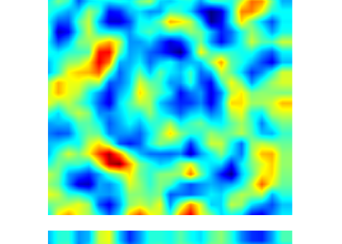
Figure 4: Realistic picture of the bubbly CMB polarization anisotropies. The simulated patch is $2^{o}\times 2^{o}$. The bubble has radius $R=20h^{-1}$ Mpc and central density contrast at decoupling $\delta=10^{-2}$ (bottom) and $\delta=5\times 10^{-3}$ (up). Together with the bubbly signal, the portion of sky simulated contains a pure CDM Gaussian one.

Now, anticipating issues of the next section, we realistically predict what we should observe in the CMB sky if a bubble was really present at decoupling on the observed patch. In figure (4) we have simulated $2^{o}\times 2^{o}$ portions of microwave sky. First look at the bottom panel. In each point we have plotted the $Q$ Stokes parameter of the CMB anisotropy. The signal consists of two components: a Gaussian scale invariant adiabatic CDM spectrum [Ma & Bertschinger 1995] and a bubble with comoving size $R=20h^{-1}$ Mpc lying exactly on the LSS ($d=0$), just like the solid line of figure (3). This case could be realistic in the sense that if during inflation more than one field were on the scene, and at least one undergoes quantum tunneling and bubble nucleation, at reheating we should expect both the kinds of perturbation of the figure, bubbly and Gaussian; also, they simply add together if the perturbations are linear. The fascinating circular imprint of the bubble is clearly visible well over the CDM contribution; the central density contrast in this case is $\delta=10^{-2}$. Note that the bubble lies on the center of the figure, within $10^{{}^{\prime}}$ from the center. The circular polarization wave is well visible and it is outside the bubble, as we have already pointed out. If $\delta$ is reduced, we go to the case of the upper panel, in which the bubble is also present, but with a smaller amplitude, $\delta=5\cdot 10^{-3}$. In this unlucky case the detection of the bubbly signal would require the use of more sophisticated image analysis tools than the human eye.

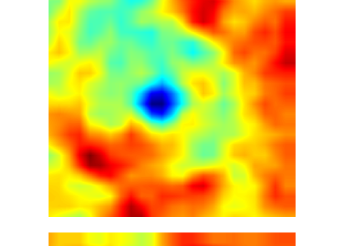
Figure 5: Realistic picture of the bubbly CMB temperature anisotropies. The simulated patch is $2^{o}\times 2^{o}$. The bubble has radius $R=20h^{-1}$ Mpc and central density contrast at decoupling $\delta=10^{-2}$ (bottom) and $\delta=5\times 10^{-3}$ (up). Together with the bubbly signal, the simulated portion of the sky contains a pure CDM Gaussian one. Note the presence of the central dark spot, absent in the polarization case.

Finally, figure (5) shows the temperature signal instead of the polarization. Note as the circular rings are well evident in the bottom panel, where $\delta$ is higher. Again, the bubble lies in the very central region, corresponding to the small central dark spot; the rings around are a feature of the CMB own physics and are coupled, for extension and oscillating behavior, with the polarization ones. The central dark spot is absent in the polarization case due to the symmetry constraints previously mentioned.

The cross detection, both in temperature and polarization anisotropies, of the CMB rings caused by a localized perturbation like a bubble would be a powerful check if signals like the present ones should be really detected in the future high resolution maps from MAP and Planck [see the Planck Surveyor and Microwave Anisotropy Probe home pages].

In the next section we consider the imprint of a population of bubbles on the CMB anisotropy power spectrum.

4 Temperature and polarization effects from a distribution of bubbles

Let us consider now a distribution of bubbles. Our purpose is to check whether, and under which hypothesis, a distribution of bubbles is able to make a distinctive imprint on the CMB angular power spectrum: let us spend a few words to recall its definition. Given a sky signal $s(\theta,\phi)$, the angular power spectrum is a set of coefficients $C_{l}$s simply defined in terms of the coefficients $a_{lm}$ of its expansion into spherical harmonics:

$$C_{l}={1\over 2l+1}\sum_{m=-l}^{m=l}|a_{lm}|^{2}\ .$$ (28)

Since it depends on the squared modules of the $a_{lm}$s coefficients, it is sensitive on the anisotropy power on the angular scale $\alpha$ roughly corresponding to $180/l$ degrees [see Padmanabhan 1993 for reviews].

This work contains some improvements with respect to previous results treating the CMB power spectrum from a distribution of bubbles [Amendola, Baccigalupi & Occhionero 1998]: first both polarization and temperature signals are computed here, and second the signals from far bubbles, namely up to a sound horizon from the LSS, are considered instead of only the closest ones at a distance of about a radius from the LSS.

We analyze $10^{o}\times 10^{o}$ zero mean CMB anisotropy maps with $3.5^{{}^{\prime}}\times 3.5^{{}^{\prime}}$ squared pixels. Bubbly signals are randomly distributed within the patch, which is projected on the sky via the Healpix pixelization [see the home page of the Healpix package], setting the signal outside the patch to zero; successively, the signal is developed into spherical harmonics using Fast Fourier Transform methods in order to get the $C_{l}$ coefficients. We analyze both maps containing only the signals from bubbles and the latter together with the CDM Gaussian perturbations as in figures 4,5.

First, in order to test our analysis method, we consider only CDM fluctuations. Starting from the theoretical CMB power spectrum, we simulate a patch as specified above and we extract from the latter the power spectrum itself, thus reconstructing the theoretical one. In figure 6 we plot the reconstructed and theoretical CDM power spectra for temperature (up) and polarization (down) anisotropies. The spectra are in quite good agreement (roughly $10\%$ accuracy) for a wide range of angular scales, corresponding to $l\geq 50$, while of course they disagree as approaching the dimension of the patch (roughly corresponding to $l\simeq 20$); the oscillations in the simulated spactra are due to the sample variance on the sky patch, but for our purpose here this method works well.

Let us define now the distribution of the bubbles. Because of the anisotropy propagation treated in the previous section, the signal on the LSS contains contributions from bubbles centered at a distance that extends up to a sound horizon $r_{s}$ at decoupling. Indicating with $R$ the radius of the bubbles, and with $x$ the fraction of volume occupied, the number of bubbles that we should consider in our patch is roughly

$$n=x\cdot 2r_{s}\cdot{3\over 4\pi R^{3}}\cdot(2H_{0}^{-1})^{2}d\Omega\ ,$$ (29)

where $d\Omega$ is the solid angle subtended by the patch in the sky and $2H_{0}^{-1}$ is the comoving distance of the LSS from us. In our simulations we adopted $R=20h^{-1}$ Mpc, so that for $r_{s}\simeq 100h^{-1}$ Mpc a $x=10\%$ volume fraction is covered by roughly 600 bubbles in the specified patch.

First, let us analyze the effect of the bubbles only. Figure 7 shows the temperature (up) and polarization (down) spectra from bubbles filling a volume from $10\%$ (thin line) to $50\%$ (heavy line). The bubbles have central density contrast at decoupling $\delta\simeq 10^{-3}$. As expected for sub-horizon structures at decoupling, the whole signal lies on sub-degree angular scales, $l\geq 200$. In the temperature case, two region can be identified: the highest one describes the central hot spot of the bubbly signals and involves the corresponding multipoles at $l\simeq 800$; while the signals vanishes rapidly higher $l$s, it shows a sort of tail that reaches $l\simeq 200$, and that is generated by the anisotropy sound waves treated in the previous section extending the signal nearly up to one degree, see figures 1,3,5. The spectrum form is completely different in the case of the polarization. This is an expected feature, since the polarization signal described in the previous section does not possess the central hot spot due to the spherical symmetry of the bubble. Instead, the polarization spectra contains peaks roughly at four angular scales that are related to the polarization waves departing from the center of the bubbles and extending up to about one degree and that are evident in figures 2,3,4.

Let us come now to the evaluation of the scalings of the CMB power induced by bubbles. In this case all the bubbles have the same central density contrast $\delta$, so that their power spectra scale exactly as $\delta^{2}$. Moreover, as expected for spatially uncorrelated bubbles, the amplitude is quite linear into the occupied volume fraction $x$. In this work we do not show graphs relative to other radii, but since the bubbles are sub-horizon structures at decoupling [see Padmanabhan 1993 for reviews], we checked that their signal scales roughly as $R^{2}$; in addition, as we mentioned in the previous section, the computation of the anisotropies causes an additional damping due to the line of sight integration across the LSS: the signal therefore drops by a factor 10 passing from $20h^{-1}$ Mpc to $10h^{-1}$ Mpc, implying a scaling of about $R^{3.5}$. Putting together all these ingredients, and defining the bubbly spectral power as $C^{T,P}=l(l+1)C_{l}^{T,P}/2\pi$ calculated roughly at the maximum, we can infer the follow empirical scalings:

$$C^{T} = 4\cdot 10^{-4}\delta^{2}\left({x\over 50\%}\right)\cdot\left({R\over 20h^{-1}{\rm Mpc}}\right)^{7}\ ,$$ (30)

$$C^{P} = 3\cdot 10^{-6}\delta^{2}\left({x\over 50\%}\right)\cdot\left({R\over 20h^{-1}{\rm Mpc}}\right)^{7}\ .$$ (31)

Note that these numbers, for what concerns temperature, lead to results that are bigger by nearly a factor of 2 than the scaling inferred previously [Amendola, Baccigalupi & Occhionero 1998]. This is probably because in our simulations more signal imprints the patch, since we considered the contributions from bubbles placed up to a CMB sound horizon away from the LSS. Since the recent measurements of CMB anisotropy power on sub-degree angular scales [see Lasenby et al. 1998, De Bernardis et al. 1998 and references therein] indicate values roughly at the level $l(l+1)C_{l}/2\pi\simeq 4\cdot 10^{-10}$ in the region interesting for us, bubbles populations with $C^{T}$ larger then that values are likely to be excluded. This implies the following constraint on our parameters:

$$\delta^{2}\left({x\over 50\%}\right)\left({R\over 20h^{-1}{\rm Mpc}}\right)^{7}\leq 10^{-6}\ .$$ (32)

This condition is obtained considering only the power from bubbles, anyway it holds also when considering the power from Gaussian CDM perturbations, simply the two perturbations mechanisms are uncorrelated, so that their powers approximatively add. Indeed, figures 8 and 9 show the CMB angular power spectra in the cases in which bubbles and CDM Gaussian perturbations are present in the simulated patch. Also plotted are the existing data on $l\geq 200$ [see Lasenby et al. 1998, De Bernardis et al. 1998 and references therein]. In figure 8 the bubbly distribution are taken from the $x=50\%$ case shown in figure 7. As we anticipated, and as it is evident looking at figures 6,7, the power from each one of the two perturbations mechanism approximatively adds. In figure 8 as example of the effect of varying $\delta$ is shown: we plotted a case in which the volume fraction is $x=10\%$ but $\delta=2\cdot 10^{-2}$. As a final comment, we wish to point out how there are cases in which the bubbles are present, filling a significant fraction of the volume and having properties able to influence the structure formation process between decoupling and the present, but that produce CMB power that is subdominant with respect to the Gaussian CDM one: this happens roughly for $C^{T}\leq 10^{-10}$, equivalent to $C^{P}\leq 10^{-12}$. This is not surprising, since in these kind of non-Gaussian models, the power spectrum alone does not fix completely the underlying perturbations properties, since, as it is evident from its definition (28), it is sensitive on the anisotropy power at a given angular scale.

5 Conclusion

The most known inflationary model leaves traces in the form of Gaussian perturbations. With these hypothesis, it uniquely marks the angular power spectrum of the cosmic microwave background (CMB) anisotropies. However high energy physics may be more complicated and may leave other (and richer) traces, in the form of non-Gaussian perturbations. During inflation, quantum tunneling phenomena may have occurred, and the nucleated bubbles may have been stretched to large and observable scales by the inflationary expansion itself. Here we predict the imprint of bubbles on the CMB, both on the polarization and temperature anisotropies. We consider an analytical bubbly density perturbation at the beginning of the radiation era, parameterized by its comoving radius $R$ and density contrast $\delta$. We perform its evolution via the linear cosmological perturbation theory. We find that it uniquely marks both the polarization and temperature anisotropies. Then we consider a parametric distribution of bubbles and we predict its imprint on the CMB angular power spectra, as a function of the bubbles abundance and properties.

During the evolution toward decoupling, we take some photos of the bubbly CMB perturbation at different times. As expected, we find that the initial condition remains unchanged until the horizon reenter occurs, and thereafter the perturbation starts to oscillate. This behavior generates sound waves propagating outward with the sound velocity of the photon-baryon fluid and reaching the sound horizon at the time we are examining the system. At decoupling, we get the CMB anisotropies by considering the bubbly perturbation intersecting the last scattering surface. The dependence of the signal on the position of the bubble along the line of sight has been considered.

The CMB polarization image of an inflationary bubble at decoupling is a series of rings concentric with the center of the bubble, extending on an angular size corresponding to the sound horizon at decoupling ($\simeq 1^{o}$ in the sky); each ring is characterized by its own value of the Stokes parameters, giving the difference of the temperature fluctuations projected on the axes parallel and perpendicular to the plane formed by the radial and photons propagation directions. As an important difference with respect to the case of temperature anisotropy, that reflects also in the CMB power spectrum from a distribution of bubbles, the light coming from the center of the bubble is not polarized, since the radial propagation in spherical symmetry is an axial symmetric problem, so that no preferred axis exists on the polarization plane. Instead, temperature anisotropies are generally characterized by a strong central spot, together to the external rings. This is an important difference, that we prepare to investigate for what concerns the impact on the CMB angular power spectrum. Finally, the amplitude of the CMB fluctuation follows the known estimates for linear perturbations with size $R$ and density contrast $\delta$: $\delta T/T\simeq\delta\cdot(R/H^{-1})^{2}$ where $\delta$ and the Hubble radius are computed at decoupling; the amplitude of the polarization is roughly 10$\%$ of the pure temperature one, as the ordinary Gaussian perturbations.

To compute the CMB power spectra induced by a population of bubbles, we simulate $10^{o}\times 10^{o}$ CMB sky patches in which they are placed randomly and fill a fraction $x$ of the volume. By taking the angular power spectrum, we analyze first the impact of the bubbles only on polarization and temperature. We find the signal lying entirely on sub-degree angular scales, characterized by a series of narrow peaks for polarization and a broader one for temperature, reflecting the signals from each bubble singularly. The amplitudes of these peaks depends in a rather simple manner by volume fraction, dimension and central density contrast of the bubbles, from which we infer an empirical formula giving the approximate bubbly CMB power; we also use this formula to constrain the bubbly distribution parameters starting from existing sub-degree CMB observations. When considering bubbles together with Gaussian fluctuations from slow roll inflation, as realistical if a bubble nucleating era occurred before the end of inflation, we find Gaussian and bubbly CMB power spectra approximatively add because of their uncorrelation.

Bubbly density perturbations are remnant of inflationary tunneling phenomena. Their detection would bring an invaluable insight into the hidden sector of high energy physics. In this work CMB bubbly signals have been computed and could be compared with the data from the future high resolution observations provided by the MAP and the Planck missions in the next decade.

The first part of this work was written at the NASA/Fermilab Astrophysics center. C.B. warmly thank the hospitality of the Theoretical Astrophysics Group. We are also grateful to Luca Amendola and Franco Occhionero for useful discussions.

We thank Eric Hivon and Krzysztof M. Gorski for their Healpix sphere pixelization that we extensively used in this work. We wish also to thank Davide Maino for his help in producing CMB maps.

Figure 1: Radial behavior of the bubbly temperature perturbation at different times. The initial condition remains unchanged until the horizon reenter occurs. The successive oscillations generate CMB perturbation propagating outward with the photon-baryon fluid sound velocity.

Figure 2: Radial behavior of the bubbly polarization perturbation at different times. The initial condition remains unchanged until the horizon reenter occurs. The successive oscillations generate CMB polarization waves propagating outward as in the pure temperature case. The substantial difference is the absence of central perturbation, because of the spherical symmetry of the perturbations.

Figure 3: Polarization (up) and temperature (down) anisotropies from bubbles with the indicated radii intersecting exactly the last scattering surface. The sound waves have been photographed by the decoupling photons in both cases. For the polarization, the central perturbation spot is absent. Thin long(short) dashed lines are anisotropies from bubbles placed at a distance $+(-)R$ with respect to the last scattering surface. Thin continue lines in the bottom panels show the signals from the two first temperature multipoles $\Theta_{0}$ and $\Theta_{1}$.

Figure 6: The theoretical (dashed line) CMB power spectra for the CDM Gaussian perturbations model adopted in this work has been simulated and reconstructed (solid line) in a $10^{o}\times 10^{o}$ sky patch. Temperature (up) and polarization (down) agree quite well for $l\geq 50$.

Figure 7: CMB temperature (up) and polarization (down) power spectra for bubbles with $R=20h^{-1}$ Mpc, $\delta=10^{-3}$ and filling volume fractions between $10\%$ (thin line) and $50\%$ (heavy line). Note how the signal is confined to sub-degree angular scales $l\geq 200$.

Figure 8: CMB temperature (up) and polarization (down) power spectra for Gaussian CDM perturbations and bubbles with $R=20h^{-1}$ Mpc, $\delta=10^{-3}$ and filling $50\%$ of the volume (heavy line). Also plotted are the purely Gaussian perturbations (thin line) and the existing experimental data on sub-degree angular scales $l\geq 200$.

Figure 9: CMB temperature (up) and polarization (down) power spectra for Gaussian CDM perturbations and bubbles with $R=20h^{-1}$ Mpc,$\delta=3\cdot 10^{-3}$ and filling $10\%$ of the volume (heavy line). Also plotted are the purely Gaussian perturbations (thin line) and the existing experimental data on sub-degree angular scales $l\geq 200$.

References

- [see Lasenby et al. 1998, De Bernardis et al. 1998 and references therein] Lasenby A.N., Jones A.W. & Dabrowski Y., 1998, proceedings of the XXXIIIrd Moriond Astrophysics Meeting, p.221; De Bernardis P. & Masi S., 1998, proceedings of the XXXIIIrd Moriond Astrophysics Meeting, p.209
-
[see the Planck Surveyor and Microwave Anisotropy
Probe home pages]
Planck Surveyor:
http://astro.estec.esa.nl/SA-general/Projects/Planck/ ;
Microwave Anisotropy Probe: http://map.gsfc.nasa.gov/ - [see the home page of the Healpix package] Healpix packadge is available at http://www.tac.dk/healpix/
- [Amendola, Baccigalupi & Occhionero 1998] Amendola L., Baccigalupi C. & Occhionero F. 1998 ApJL 492, L5
- [Baccigalupi et al. 1997] Baccigalupi C., Amendola L. and Occhionero F. 1997, MNRAS 288, 387
- [Baccigalupi 1998] Baccigalupi C. 1998, ApJ 496 615, astro-ph/9711095
- [Baccigalupi 1999] Baccigalupi C. 1999, Phys.Rev.D59, 123004, astro-ph/9811176; see also Baccigalupi C. 1999, astro-ph/9901040
- [Ma & Bertschinger 1995] Ma & Bertschinger 1995, ApJ 455, 7; Kodama I. & Sasaki M. 1984, Progr.Theor.Phys.Supp. 78, 1; Bardeen J.M. 1980, Phys.Rev.D 22, 1882
- [Hu et al. 1997] Hu W., Seljak U., White M. & Zaldarriaga M. 1997, Phys.Rev.D 56, 596, astro-ph/9709066; Hu W. & White M. 1997 Phys.Rev.D 56, 596, astro-ph/9702170
- [see Hu & Sugiyama 1995 for useful fitting formulas] Hu W. & Sugiyama N. 1995, Ap.J. 444, 489, astro-ph/9407093
- [El-Ad, Piran & da Costa, 1997] El-Ad H., Piran T. & da Costa L. N. 1997, MNRAS 287, 790; El-Ad H., Piran T. & da Costa L. N. 1996, ApJL 462, L13
- [see Amendola et al. 1996 and references therein] Amendola L., Baccigalupi C., Konoplich R., Occhionero F., Rubin S. 1996, Phys.Rev.D 50, 4846; Turner M.S., Weinberg E.J. & Widrow L.M. 1992, Phys.Rev.D 46, 2384; La D. 1991, Phys. Lett. B 265, 232
- [see Kolb 1991 and references therein] Kolb E.W. 1991, Physica Scripta T36, 199
- [see Mukhanov, Feldman & Branderberger 1992 for an extensive treatment] Mukhanov V.F., Feldman H.A. & Branderberger R.H. 1992, Phys.Rep. 215, 203
- [Occhionero et al. 1998] Occhionero F., Baccigalupi C., Amendola L. & Monastra S. 1998, Phys.Rev.D56, 7588
- [see Padmanabhan 1993 for reviews] Padmanabhan T. 1993, Structure Formation in the Universe, Cambridge University Press editions