BOOMERanG: a scanning telescope
for 10 arcminutes resolution CMB maps

Abstract

The BOOMERanG experiment is a stratospheric balloon telescope intended to measure the Cosmic Microwave Background anisotropy at angular scales between a few degrees and ten arcminutes. The experiment features a wide focal plane with 16 detectors in the frequency bands centered at 90, 150, 220, 400 GHz, with FWHM ranging between 18 and 10 arcmin. It will be flown on a long duration (7-14 days) flight circumnavigating Antarctica at the end of 1998. The instrument was flown with a reduced focal plane (6 detectors, 90 and 150 GHz bands, 25 to 15 arcmin FWHM) on a qualification flight from Texas, in August 1997. A wide ($\sim$ 300 deg², i.e. about 5000 independent beams at 150 GHz) sky area was mapped in the constellations of Capricornus, Aquarius, Cetus, with very low foreground contamination. The instrument was calibrated using the CMB dipole and observations of Jupiter. The LDB version of the instrument has been qualified and shipped to Antarctica.

Introduction

The target of the BOOMERanG experiment is to make $\ell$-space spectroscopy of the power spectrum of CMB anisotropies in the region of the first three acoustic peaks ($50\lower 2.15277pt\hbox{$\;\buildrel<\over{\sim}\;$}\ell\lower 2.15277pt\hbox{$\;\buildrel<\over{\sim}\;$}800$). This will be obtained by multiband mapping of wide ($\;\buildrel>\over{\sim}\;$ 20000 independent pixels ) sky regions in the lowest foreground areas, with angular resolution approaching 10 arcmin FWHM and with S/N per pixel $\lower 2.15277pt\hbox{$\;\buildrel>\over{\sim}\;$}1$. This target can be achieved with a scanning instrument. This class of instruments features a number of nice properties:

$\bullet$ It allows simultaneous measurements of the CMB anisotropy spectrum over a wide $\ell$ range, with reasonable $\ell$ resolution;

$\bullet$ No moving parts are necessary in the optical system, thus achieving high reliability and avoiding offsets from chopper-synchronous signals;

$\bullet$ Such an instrument is a testbed for future satellites using similar technologies and observation strategies, like Planck Surveyor.

Moreover, the experiment can be sub-orbital, due to recent progress in different areas:

$\bullet$ development of very fast and sensitive bolometric detectors and readout electronics with very low 1/f noise;

$\bullet$ development of low-background, low-sidelobes microwave telescopes;

$\bullet$ Long Duration Ballooning opportunities and related payload technologies (CR immune hardware, stable readout, long duration cryogenics, stable scan-oriented attitude control system.)

The quest for good angular resolution in CMB anisotropy measurements, with the practical need for a reasonable telescope size, drive us towards high frequencies, i.e. bolometric techniques. In fact a beam FWHM of about 10 arcmin requires a telescope diameter $D\sim 3m$ in the best operation band of HEMTs (around 40 GHz), while $D\sim 1m$ at 150 GHz, a good operation band for modern composite bolometers. High frequencies require a balloon experiment to avoid most of the atmospheric emission, thus achieving low background on the bolometers and low atmospheric noise. This can be obtained only with correct optical filtering, an extremely difficult and important issue of millimeter-wave bolometric photometry. The quest for repeated mesurements, allowing deep checks for systematic effects, drives us to long (few days) balloon flights. Long Duration Ballooning is carried out by NASA-NSBF in Antarctica. In the case of CMB anisotropy experiments the advantages are as follows:

$\bullet$ the long duration (7-14 days) provides the opportunity to check extensively for systematic effects, the most troublesome source of errors in this type of measurements;

$\bullet$ the long integration time per pixel gives high sensitivity, making CMB mapping possible over significant sky fractions;

$\bullet$ the sun, always present, provides power supply through solar panels and a stable thermal environment.

Disadvantages are also present, as listed below:

$\bullet$ the increased cosmic rays density in polar regions requires special, custom developed detectors;

$\bullet$ the long duration requires special cryogenic systems;

$\bullet$ the presence of the sun restricts the observations to the antisolar regions, requires multiple sun shields to produce a thermally stable telescope and requires very low sidelobes (-90 dB at 180^o) for the telescope;

$\bullet$ the payload is not always in the line of sight of the telemetry base, so special communications are required, and the interactivity with the instrument can be somewhat reduced.

We have developed and tested a payload Lange1 , Paolo1 , Silvia1 , which takes full advantage of the opportunities listed above for LDB flights, and efficiently takes care of all the related problems. The instrument is called BOOMERanG (Balloon Observations Of Extragalactic Radiation and Geophysics).

Observation Strategy

BOOMERanG is a scanning experiment: the beam scans the sky at constant elevation and constant azimuth speed. Different spherical harmonic components of the temperature field produce different electrical frequencies in the detector. So, in principle, $\ell$-space spectroscopy is possible using a scanning instrument and an averaging signal analyzer. This experimental approach has been made possible by the development of the latest generation ultra-sensitive bolometers, achieving a noise of $\sim 100\mu K_{CMB}\sqrt{s}$. In the case of scans along circles (constant elevation or declination) there is a simple relationship between the Fourier spectrum of temperature fluctuations measured along each circle and the usual spherical harmonic expansion coefficients on the sphere ($C_{l}$) (delab ). Given the azimuth $\phi$, the colatitude $\theta_{o}$ (constant along the circle), and the measured CMB temperature $T(\theta_{o},\phi)$ we define the Fourier transform of the CMB temperature measured along the scan

$$\alpha_{m}={1\over 2\pi}\int_{0}^{2\pi}T(\theta_{o},\phi)e^{-im\phi}d\phi$$

and the 1-D power spectrum of the temperature fluctuations

$$\delta_{mm^{\prime}}\Gamma_{m}=\left<\alpha_{m}\alpha^{*}_{m^{\prime}}\right>$$

It can be shown that

$$\Gamma_{m}=\sum_{l=|m|}^{\infty}C_{l}B_{l}^{2}{\cal P}_{l,m}^{2}(\theta)$$

This quantity is to be compared to the power spectra of the time series of the signal detected by the scanning CMB telescope. The $m$ component of the 1-D spectrum will produce an electrical signal in the CMB detector at a frequency

$$f={{\dot{\phi}}\over 2\pi}m$$

The scan speed ${\dot{\phi}}$ must be optimized in such a way that the interesting $m$ range (in our case, the region of the acoustic peaks) is detected in a frequency range far from 1/f noise, interferences,and detector roll-off effects. In fig.1 we compare the system noise (including atmospheric effects induced by payload pendulations) to the 1-D power spectrum of CMB anisotropies, assuming two different scan speeds and a 12 arcmin FWHM gaussian beam. It is evident that with a suitable choice of the scan speed ($\lower 2.15277pt\hbox{$\;\buildrel>\over{\sim}\;$}2deg/s$) the interesting features in the CMB power spectrum can be observed in a frequency range where detector noise is reasonably flat.

Figure 1: 1-D power spectrum of CMB anisotropies (multiplied by the beam MTF for a 12 arcmin FWHM gaussian beam) compared to system noise for a scanning experiment. The goal of the optimization process is to move the interesting spectral features of the signal (the ”acoustic peaks” in our case) in the frequency range where the experiment noise is flat and low. A scan speed of $\lower 2.15277pt\hbox{$\;\buildrel>\over{\sim}\;$}2^{o}/s$ is required to avoid 1/f noise and pendulation features.

During a day-time LDB flight the payload can observe only a restricted region opposite to the sun. The BOOMERanG payload makes inversion smoothed triangular-wave azimuth scans, 60 deg peak to peak, at constant elevation. This can be selected in the range $40^{o}\lower 2.15277pt\hbox{$\;\buildrel<\over{\sim}\;$}e\lower 2.15277pt\hbox{$\;\buildrel<\over{\sim}\;$}50^{o}$.

For the LDB flight the azimuth scan is centered on the Horologium constellation, the minimum foreground region in the IRAS-DIRBE maps Schl , which happens to be close to the anti-sun direction during the LDB flights performed in the antarctic summer. In this region the expected foreground fluctuation is of the order of a few microkelvin CMB at 150 GHz.

This strategy provides us with a wide sky map (about 40 deg wide by 30 deg high). The full map is observed once per day for several days. The flight path is approximately a circle at constant latitude ($\sim 80^{o}$ south). The longitude drift of the experiment during the flight produces a variable tilt of the scan direction in the RA-dec plane, thus providing usefull cross linking in the dataset.

The focal plane of the experiment features two 4 x 4 arrays of photometers (see fig.2).

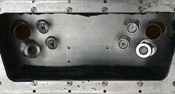
Figure 2: Photograph of the BOOMERanG focal plane array of receiver horns. The input diameter of the smaller horns is 6 mm. The horns correspond to the following channels: top row: B90A, BXXXA1, BXXXB1, B90B; bottom row: B150A, BXXXA2, BXXXB2, B150B. The numbers here label the operating fequency in GHz for single mode horns; XXX is the input of a 3-color (150, 220, 400 GHz) photometer.

So we have three levels of sources (or structures) confirmation: after the first scan, the reversed time domain structure must be evident in the signal from the same detector scanning back to the start position after few tens of seconds; moreover the same structure must be evident in the symmetric detector with the same frequency band active in the same row of the considered one (first level confirmation). The same structure must be evident in the signals from the second row of detectors, scanning the same sky strip a few minutes after the first row, due to the daily sky rotation (second level confirmation). The same structure must be evident in the signals from the scans measured the subsequent day at the same time (Third level confirmation). First and second level confirmations are effective in discerning sky signals from system instabilities (thermal or radiofrequency), atmospheric fluctuations and scan synchronous effects; third level confirmation is useful to discern sky signals from sidelobes artifacts (ground or sun pick-up).

Our instrument features multiband photometers. This allows us to analyze spectrally the detected structure, comparing it to the structures seen in the other spectral bands. This is an extremely powerful method to recognize the spectral signature of CMB anisotropies, which is greatly different from that of dust and synchrotron foregrounds and from that of atmospheric emission.

The Instrument

The BOOMERANG experiment is a millimeter wave telescope, with a bolometric receiver working in a long-duration cryostat at 0.3 K for 15 days. The instrument is part of the BOOMERanG/MAXIMA collaboration, sharing similar basic technologies (detectors and ACS, see the paper from A. Lee in these proceedings). BOOMERanG has been optimized for the peculiar requirements of Antarctic long duration ballooning (LDB). A diagram of the optical system is presented in fig.3. The primary mirror of the telescope (a 1.3 m diameter, 1.5 m focal length, off-axis paraboloid) is at ambient temperature. It is made out of 6061 aluminum, as is the entire telescope frame. At the focus of this telescope, the multiband receiver features beams ranging from 12 to 20 arcmin FWHM (depending on the channel and on the configuration). The telescope is protected by an earth shield and by two large sun shields, which allow operation of the system in the range $\pm 60^{o}$ from the anti-solar azimuth. Off axis radiation at 150 GHz is undetected at the -85dB level. The secondary and tertiary mirrors are cooled to 2K inside the cryostat. Radiation enters the cryostat through a 50 $\mu m$ thick polypropylene window, and goes through blocking filters at 77K and at 4.2K. The tertiary mirror is the cold Lyot stop of the instrument, sharply limiting the field of view of the photometers. Throat-to-throat concentrators with their entrance aperture placed in the telescope focal plane allow radiation to enter inside the RF-tight box containing the ³He refrigerator and the detectors. The detectors use parabolic and conical concentrators, metal mesh filters and Si₃N₄ spider web absorber bolometers. A photograph of the focal plane array for the Antarctic flight and of its ancillary hardware is shown in fig.3.

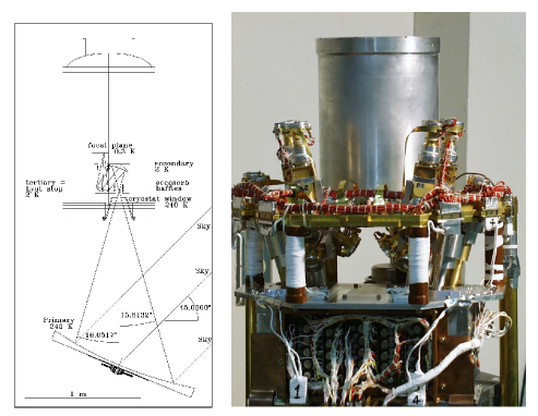
Figure 3: Optical layout of the instrument (left) and photo of the focal plane array for the LDB flight. The multiband photometer arrays are visible, mounted on the 0.3 K flange. The 0.3K stage is mounted on four vespel columns over the cold FET stage visible in the lower part of the picture. The long duration ³He fridge is visible behind the detectors. The height of the cold insert shown in the picture is 50 cm.

We have two different configurations for the focal plane. For the short test flight we traded angular resolution for throughput in order to get significant sensitivity during the short flight from Texas (6 hours). The final configuration, used for the Antarctic flight, has higher angular resolution and improved detectors (see fig.2 and 3). Low background bolometers are extremely sensitive to all forms of radiant energy. One big problem with standard bolometers is energy deposition from cosmic rays (CR) particles. Previous experiments carried out in temperate regions measured typical rates of an event every few seconds. The problem is enhanced in the polar stratosphere, where we expect a flux of cosmic rays about 6 times larger than in the temperate stratosphere. Bolometers with negligible cross sections for cosmic rays have been developed bock , Mausk and tested in flight. The absorber is a thin web ($\sim 1\mu m$ thickness) micromachined from Si₃N₄ and metalized. The grid constant is of the order of a few hundred microns, smaller than the in band wavelength so that photons are effectively absorbed while CR are not. Also the heat capacity of the bolometer is greatly reduced, and the mechanical resonant frequency is in kHz range. NEPs of the order of $10^{-17}W/\sqrt{Hz}$ at 0.3K are achieved with time constants of the order of 10 ms for the 150GHz detectors. The other form of energy which contaminates signals from high sensitivity bolometers is radio frequency (RF) pickup, either through the optical path or through the readout circuit. This problem is very severe in the case of balloon borne payloads, which have powerful GHz telemetry transmitters on board. The BOOMERanG receiver has been carefully shielded: all the detectors operate in a RF tight cavity. Millimeter-wave radiation enters the cavity through apertures much smaller than the RF wavelength (inside the throat to throat parabolic concentrators), and all the wires enter the cavity through cryogenic EMI filter feedthroughs. Similar care has been taken for the signal processing circuits.

The bolometers are differentially AC biased and read-out. The bolometer signals are demodulated by lock-ins synchronous with the bias voltages. A RC cut-off at a frequency (15 mHz) lower than the scan frequency was used to limit the dynamical range of the data and to remove 1/f noise from very low frequencies, unimportant for our measurements.

A long duration ${}^{4}He$ cryostat MasiB cooling the experimental insert to 2K, and a long duration ${}^{3}He$ fridge MasiA , cooling the photometers to 280 mK, have been developed. The cryostat has a central 50 liter volume available for the 2K hardware, including blocking filters, secondary and tertiary mirrors, cryogenic preamplifiers, back to back concentrators, ³He fridge, and photometers. The cryogens hold time exceeds 12 days under flight conditions.

The telescope and receiver hardware are mounted on a tiltable frame (the inner frame of the payload). The observed elevation can be selected by tilting the inner frame by means of a linear actuator. The outer frame of the payload is connected to the flight train through an azimuth pivot. The observed azimuth can be selected by rotating the full gondola around the pivot, by means of two torque motors. The first actuates a flywheel, while the second torques directly against the flight train. An oil damper fights against pendulations induced by stratospheric wind shear or other perturbations. The sensors for attitude control are different for night-time flights (like the test flight in 1997) than day-time flights (like the Antarctic flight in 1998). For the night-time flight in Texas we had a set of 3 vibrating gyroscopes and a flux-gate magnetometer in the feedback loop driving the sky scan. A CCD camera with real-time star position measurement provides attitude reconstruction to 1 arcmin. For the day-time flight in Antarctica we have a coarse and a fine sun sensor, a differential GPS, and a set of 3 laser gyroscopes. Again, we expect to be able to reconstruct the attitude better than 1 arcmin.

THE TEST FLIGHT

The system was flown for 6 hours on Aug 30, 1997, from the National Scientific Balloon Facility in Palestine, Texas. All the subsystems performed well during the flight: the He vent valve was opened at float and was closed at termination, the Nitrogen bath was pressurized to 1000 mbar, the ³He fridge temperature (290mK) drifted with the ⁴He temperature by less than 6mK during the flight. Pendulations were not generated during CMB scans, at a level greater than 0.5 arcmin, and both azimuth scans at 2^o/s and full azimuth rotations (at 2 and 3 rpm) of the payload were performed effectively. The loading on the bolometers was as expected, and the bolometers were effectively CR immune, with white noise ranging between 200 and 300 $\mu K\sqrt{s}$ depending on the channel. During the flight, the system observed Jupiter to measure the beam pattern and responsivity. A strip of sky at high galactic latitudes ($\sim$ 4 deg high in declination, $\sim$ 6 hours wide in RA) in the constellations of Sagittarius, Capricornus, Aquarius, and Sculptor, was scanned in search for CMB anisotropies. The gondola performed 40^o peak to peak azimuth scans, centered on the south, with 50 s period, for 5 hours. Sample scans are shown in fig.4. The signal from the pitch gyroscope is fourier analyzed in fig.5, showing very small pendulations of the system.

Figure 4: Azimuth scans of the instrument during the test flight. The scans are centered around south. The earth rotation during the 5 hours of scans produced an elongated sky coverage, 4 degrees high in declination, ranging from $\sim$ 10 to 80 degrees of Galactic latitude.

Figure 5: Fourier Transform of the pitch rate gyroscope during the regular (40^op-p) azimuth scans of the instrument. The pendulations induced during the scans are very small.

IN-FLIGHT CALIBRATION

The bolometers time constants turned out to be quite long (several tens of ms) in the test flight, and we performed a careful analysis of the instrument transfer function to take care of these effects. The electronics (AC bias readout) transfer function was measured accurately and found to be very stable with temperature. The transfer function of the bolometers depends on the reference bath temperature and on the radiative loading, so in principle can change at float. It has been measured in flight with two independent methods. The first one is using cosmic rays hits. We have a few samples (60 hits in 6 hours in B150B2). They are extremely reproducible, can be normalized and synchronized. The Fourier Transform of the impulse response gives us the total (bolometer + readout electronics) transfer function of the instrument. To check that the results of this method are not confused by ionization effects, we used a second method, i.e. we analyzed the signals from fast scans (18${}^{o}/s$) on Jupiter. Here we have purely optical pulses on the bolometers. Simulation shows that beam size and beam shape effects are negligible. So we use the Fourier transform of these pulses to get the instrument transfer function. From these data we can recover $\tau_{bol}$, better than 10$\%$. This is completely acceptable, since the calibration measurements are quite unsensitive to $\tau_{bol}$. In fact, the instrument was calibrated using the amplitude of the signals observed during regular ($\sim 2^{o}/s$) scans on Jupiter. The calibration constant is

$${\mathcal{K}}={\Delta V_{planet}\over T_{CMB}}{\Omega\over\Omega_{planet}}{\int E(\nu)BB(T_{CMB},\nu){xe^{x}\over e^{x}-1}d\nu\over\int E(\nu)BB(T_{eff},\nu)d\nu}$$

with obvious meaning of the symbols. The measured $\Delta V_{planet}$ and $\Omega$ have opposite dependance on $\tau_{bol}$, so ${\mathcal{K}}$ changes by less than 1 $\%$ for a 20 $\%$ change of $\tau_{bol}$. We also checked with simulations that our deconvolution from the instrument transfer function does not affect significantly the shape and value of CMB anisotropy signals in our detectors (see aquila1 ). In fig.6 we plot an example of signal from scans on Jupiter.

Figure 6: Sample real time signals during azimuth scans on Jupiter. The scan speed is 1.7${}^{o}/s$ towards increasing azimuth, the elevation of the beam is 39^o. Due to the non-negligible time constant of the bolometers, the signals are non-symmetric. The effect of the high-pass filter is also evident in the baseline. These effects are removed by deconvolution from system transfer function in the data analysis. The forward and reverse scans shown here are different due to the sky rotation and different payload attitude.

The responsivity calibration has been obtained with the following sequence of steps: signals are deconvolved from the electronics readout and bolometer time constant, and then is filtered using a flat phase numeric filter to reduce white noise and cut drifts. The best parameters for the filter are obtained with numerical simulations. The filtered data are binned on a grid centered on the optical position of Jupiter. The beam solid angle $\Omega$ is computed by 2-D integration of the binned data. We get FWHM of 19.5, 19.5, 16.5, 24, 29 arcmin for the B150A1, B150B1, B150B2, B90A, B90B channels respectively. $\Delta V_{Jupiter}$ is estimated making fits to the scan data. ${\mathcal{K}}$ is derived using the measured quantities and the spectral information $E(\nu)$ as measured in the laboratory. Errors are propagated. The final precision of the calibration ${\mathcal{K}}$ is 5.9, 8.7, 3.8, 7.0, 5.2 $\%$ for the B150A1, B150B1, B150B2, B90A, B90B channels respectively.

An independent method of calibration for ${\mathcal{K}}$ is the observation of the CMB Dipole. In fact, the Dipole has the same spectrum as smaller scale CMB anisotropies, fills the beam, and its amplitude and direction are well known from COBE-DMR (better than 1$\%$). The Dipole was observed during the test flight for four times, to check unambiguously the celestial nature of the signal. On our scans, the expected Dipole signal ranged between 2 and 4 mK_CMB peak to peak, depending on the scan. We do see a Dipole signal in all the 90 and 150 GHz channels. The signal is not correlated to the (small) pendulations sensed by the pitch and roll gyroscopes, and rotates with the sky, thus excluding any atmospheric origin. In fig.7 we plot sample observed signals during one of the azimuth spins of the payload.

Figure 7: Data from the active detectors during the 3 rpm rotations of the payload. Nine rotations of the payload are shown. The CMB dipole signal is evident in all the channels.

Figure 8: 90 GHz data binned in angle from the DMR CMB dipole direction, are plotted versus the theoretical Dipole signal (rotation 2).

In fig.8 we plot the observed signals averaged in dipole angle bins versus the COBE-DMR dipole for channel B90B. The calibration ${\mathcal{K}}_{D}$ (derived as the ratio between the observed dipole and the COBE-DMR dipole on the same path) agrees well with the ${\mathcal{K}}$ measured from Jupiter at the same time. The final precision of the calibration for the first rotation is: $2,4,6,4,3\%$ for the B90A, B90B, B150A1, B150B1, B150B2 channels respectively. Calibration drifts are evident from both the Dipole signals and from the internal calibrator lamp, which flashed every 15 minutes and can be used as a calibration transfer during the entire flight. In summary, we estimate that our total calibration error is significantly less than 10$\%$ for all the active channels.

CMB DATA ANALYSIS PIPELINE

The $\sim 1.5\times 10^{6}$ samples are first edited removing cosmic rays hits, calibration lamp flashes, microphonic events from the nitrogen pressurization system, radar hits, signals from Jupiter, data taken in rotation mode. This editing removes less than 5$\%$ of the data. The resulting data set is mainly noise, and is stationary: the rms changes less than 2$\%$ from hour to hour. Then the data are filtered in the time domain: they are deconvolved and flat phase filtered as described in the previous paragraph; a notch filter at 6.8 Hz is applied to remove temperature control bias aliases where needed. The following steps are part of a loop which is repeated under different assumptions (forward or reverse scans, flight sections with different environment, etc.) to check for systematic effects. The noise matrix is estimated from the power spectrum of the data. The CMB analysis continues along two parallel paths. Along the first one, data are binned using synthesized beam patterns (as in Net ), and the corresponding window functions and the covariance matrix of the data are computed. A likelihood analysis produces band-power estimates of the $c_{\ell}$. Along the second path an ”optimal” map is created from the data stream following the procedures described in map , and the $c_{\ell}$ power spectrum is computed from the map (see e.g. the papers from Borrill and Jaffe in these proceedings). All this is repeated with different data selection rules, deconvolution parameters, noise estimate etc., to check for systematic effects. The procedure is applied to all the channels and to the dark channel, and correlation analysis are carried out to check for other systematic effects. It is worth to stress the following facts: the BOOMERanG 1997 data set produces a 26000 pixels map (6 arcmin pixelization with a 15 arcmin FWHM beam). At the moment, this is the biggest CMB map ever made. At the pixel level, the map is dominated by noise. The map contains both dusty sections (closer to the Galactic plane) and clean sections (up to $b\sim 80^{o}$). Both are interesting. Power spectra have been made, and we do have significant detections of CMB anisotropies in the range $50\lower 2.15277pt\hbox{$\;\buildrel<\over{\sim}\;$}\ell\lower 2.15277pt\hbox{$\;\buildrel<\over{\sim}\;$}400$. The data are sample variance limited in this range. We are in the middle of the ”check for systematics loop” process, so we cannot give final results yet. However, the two methods outlined give consistent results for the measured $c_{\ell}$s.

THE LDB FLIGHT

BOOMERanG-LDB has been qualified for flight on Aug. 25, 1997. A photograph of the payload during the qualification is visible in fig.9.

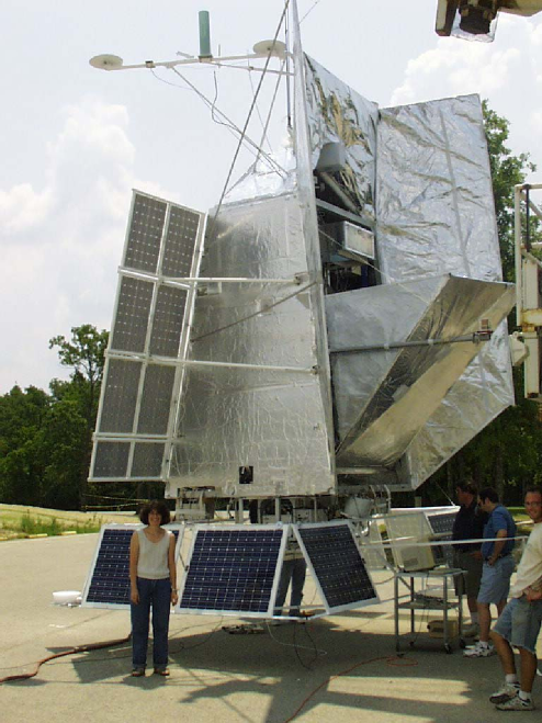
Figure 9: The BOOMERanG LDB payload during the qualification test at the NASA-NSBF in Palestine (Texas) on August 25, 1997. The earth shield and the sun shields dominate the scene. Also the solar array providing the power supply for the payload (upper) and for the navigation hardware (lower) are evident. The payload is 5.2 m high and the total weight is $\sim 1.5$ ton.

The main differences with respect to the BOOMERanG-NA, are the new focal plane and the improved detectors. Now the measured time constant for the detectors range between 16 ms (for the 90 GHz channels) and 2 ms (for the 400GHz channels). Coarse and Fine Sun sensors have been developed and calibrated for pointing reconstruction. The gyroscopes driving the scan have been replaced with optical fiber ones, featuring very low drift. The main sensors for pointing reconstruction, resetting the rate gyroscopes, are the fine sun sensors, two digital sundial featuring subarcminute resolution with a measurement range of $\lower 2.15277pt\hbox{$\;\buildrel>\over{\sim}\;$}120^{o}$ in azimuth and 50^o in elevation. A differential GPS completes the sensors set. An array of solar panels, providing $\sim 2kW$ of maximum power, has been implemented on the payload. Real time monitoring of most of the instrument signals will be possible during all the LDB flight using the TDRSS satellites constellation. The instrument will be calibrated against several HII regions visible in the southern Hemisphere, close to the main target of the instrument, the Horologium constellation, and far from the Sun. The same regions will be mapped from ground using the SUZIE instrument.

CONCLUSIONS

The test flight of the BOOMERanG experiment has demonstrated the good performance of the instrument and has qualified it for the LDB flight. The instrument has been precisely calibrated and CMB anisotropies have been detected in the range of the first acoustic peak of the $c_{\ell}$ spectrum. The data analysis pipeline has been developed, and we are currently performing deep checks for systematic effects. The LDB instrument has been shipped to Antarctica for flight at the end of 1998.

References

- (1) Delabrouille J., Gorski K.M., Hivon E., Mon. Not. Roy. Astron. Soc. 298, 445 (1998).
- (2) Lange et al. Space Science Rev.,74, 1-2, (1995)
- (3) de Bernardis et al., proceedings of the meeting Microwave Background Anisotropies, Moriond Astrophysics Meeting, F. Bouchet editor, Ed. Frontieres, 1996, pg. 155.
- (4) Masi et al. Proceedings of the workshop Topological Defects in Cosmology, Rome, 1996, M. Signore and F. Melchiorri editors (World Scientific)
- (5) D.J. Schlegel, D.P. Finkbeiner, M. Davis, ApJ, 500, 525, 20
- (6) Bock J., Chen P., Mauskopf P., Lange A., A novel bolometer for infrared and millimeter-wave astrophysics, Space Sci. Rev., 74, 229-235, 1995
- (7) Mauskopf P., et al., Composite infrared bolometers with micromesh absorbers, Applied Optics, 36, 765-771, 1997.
- (8) S. Masi, E. Aquilini, P. Cardoni, P. de Bernardis, L. Martinis, F. Scaramuzzi, D. Sforna, Cryogenics, 38, 319-324, 1998A
- (9) S. Masi, P. Cardoni, P. de Bernardis, F. Piacentini, A. Raccanelli, F. Scaramuzzi, ”A long duration cryostat suitable for balloon borne photometry” 1999, Cryogenics, in press
- (10) P. de Bernardis, G. De Troia, L. Miglio, 1999, Proc. of the International School of Space Science: coures ”3K Cosmology from Space”, F. Melchiorri, M. Signore, P. Richards, G. Sironi editors, Elsevier.
- (11) Netterfield C.B. et al., Ap.J., 474, 47, 1997
- (12) see e.g. Janssen, astro-ph 9602009, Wright astro-ph 9612006, Smoot astro-ph 9704193, Tegmark astro-ph 9711076.