CMB ANISOTROPIES DUE TO FEEDBACK-REGULATED INHOMOGENEOUS REIONIZATION

Abstract

We calculate the secondary anisotropies in the CMB produced by inhomogeneous reionization from simulations in which the effects of radiative and stellar feedback effects on galaxy formation have been included. This allows to self-consistently determine the beginning ($z_{i}\approx 30$), the duration ($\delta z\approx 20$) and the (nonlinear) evolution of the reionization process for a critical density CDM model. In addition, from the simulated spatial distribution of ionized regions, we are able to calculate the evolution of the two-point ionization correlation function, $C_{\chi}$, and obtain the power spectrum of the anisotropies, $C_{\ell}$, in the range $5000<\ell<10^{6}$. The power spectrum has a broad maximum around $\ell\approx 30000$, where it reaches the value $2\times 10^{-12}$. We also show that the angular correlation function $C(\theta)$ is not Gaussian, but at separation angles $\theta\lower 2.15277pt\hbox{$\;\buildrel<\over{\sim}\;$}10^{-4}$ rad it can be approximated by a modified Lorentzian shape; at larger separations an anticorrelation signal is predicted. Detection of signals as above will be possible with future mm-wavelength interferometers like ALMA, which appears as an optimum instrument to search for signatures of inhomogeneous reionization.

1 INTRODUCTION

At $z\approx 1100$ the intergalactic medium recombined and remained neutral until the first sources of ionizing radiation form and begin to reionize it. Current models of cosmic structure formation predict that the first collapsed, luminous objects should have formed at redshift $z\approx 30$. This conclusion is reached by requiring that the cooling time $t_{c}$ of the gas be shorter than the Hubble time $t_{H}$ at the formation epoch. The ionizing flux from these objects creates cosmological HII regions in the surrounding IGM, whose sizes are much smaller than their typical interdistance (Ciardi, Ferrara & Abel 1999). This implies that reionization passed through a highly inhomogeneous phase which ended only when the individual HII regions overlapped, or stated differently, when reionization was complete. There is essentially no direct observational test of both the beginning and the duration of the reionization process. The most stringent upper limits on the reionization redshift and the Thomson optical depth of the cosmic medium, derived from data on “linear” anisotropies at $\ell<10^{3}$, are quite model-dependent (De Bernardis et al. 1997, Griffiths et al. 1999).

However, if reionization was indeed inhomogeneous, it should have left an inprint in the CMB. In the homogeneous case, small-scale secondary anisotropies generated by Doppler effect from Thomson scattering off IGM electrons would be erased due to potential flow cancellation effects. In the inhomogeneous case, the modulation of the ionization fraction, playing a similar role as the density modulation for the nonlinear Vishniac effect, prevents such cancellation leading to anisotropies at sub-degree scales. A few papers have recently tackled the calculation of secondary anisotropies produced by inhomogeneous reionization (Aghanim et al.  1996 [see also Erratum (1999)], Knox, Scoccimarro & Dodelson 1998, Gruzinov & Hu 1998, Peebles & Juszkiewicz 1998, Haiman & Knox 1999, Hu 1999). These models are based on simple assumptions concerning the evolution of the mean ionization level, the typical size of the ionized patches and, in some cases, their spatial and redshift correlation.

Our aim here is to improve the modelling by self-consistently calculating secondary anisotropies from dedicated reionization simulations presented in Ciardi, Ferrara, Governato & Jenkins (1999, CFGJ), in which the effects of radiative and stellar feedback effects on galaxy formation have been included. Similar reionization simulations have been performed also by Gnedin (1998, 1999). This allows us to calculate the history and correlation properties of reionization to an unprecedented detail level.

2 INHOMOGENEOUS REIONIZATION

The predictions for the CMB anisotropies presented in this paper are based on the study of inhomogeneous reionization (IHR) presented by CFGJ. Although the detailed description of the model can be found in that paper, it is useful to recall here its essential features and the results relevant for the present work.

The reionization process is studied in a critical density CDM universe ($\Omega_{0}=1$, $h=0.5$ with $\sigma_{8}=0.6$ at $z=0$ and $\Omega_{b}=0.06$) as due to stellar sources, including Population III objects. The spatial distribution of the sources is obtained from high-resolution numerical N-body simulations within a periodic box of comoving length $L=2.55h^{-1}$ Mpc. The source properties are calculated taking into account a self-consistent treatment of both radiative (i.e. ionizing and H₂–photodissociating photons) and stellar (i.e. SN explosions) feedbacks regulated by massive stars. This allows, in particular, to derive the spatial distribution of the ionized regions at various cosmic epochs and the evolution of the mean H ionization. In brief, there are two main free parameters in the simulations: (i) the fraction of total baryons converted into stars $f_{b\star}$, and (ii) the escape fraction of ionizing photons, $f_{esc}$, from a given galaxy; a critical discussion of these parameters is given in CFGJ. Four different combinations of these parameters in runs A ($f_{b\star}=0.012,f_{esc}=0.2$), B (0.004, 0.2), C (0.15, 0.2) and D (0.012, 0.1) have been explored. Run A gives the best agreement between the derived evolution of the cosmic star formation rate and the experimentally deduced one at $z\lower 2.15277pt\hbox{$\;\buildrel<\over{\sim}\;$}4$ (Steidel et al. 1998, CFGJ). Therefore, here we only present results for this case.

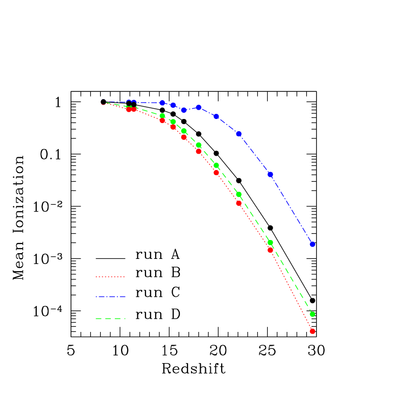
Figure 2:  Evolution of the volume-averaged mean ionization, $\bar{\chi}(z)$, for the four runs A, B, C, D whose parameters are given in the text.

The topological structure of ionization at $z=19.8$ for run A is shown in Fig. 1. The proper size of ionized bubbles is approximately in the range 1 - 20 kpc at this epoch, as only relatively small, and hence faint, objects have collapsed; they grow in number and volume with cosmic time. A more global view of the reionization process is given in Fig. 2, where the redshift evolution of the volume-averaged mean ionization fraction, $\bar{\chi}(z)$ is shown for the four different runs. Except for run C (high star formation efficiency), when reionization is complete at $z\approx 15$, primordial galaxies are able to reionize the IGM at a redshift $z\approx 10$. Note that reionization begins at $z_{i}\approx 30$ when the conditions of the cosmic medium allow the first Pop III objects to start to form, and it is then completed after a redshift interval $\delta z\approx 20$ thanks to the contribution of larger objects with mass $\approx 10^{8}M_{\odot}$.

3 SECONDARY ANISOTROPIES

To calculate the secondary anisotropies produced by IHR, we use the same method outlined by Knox et al. (1998) and Gruzinov & Hu (1998). The solution of the Boltzmann equation for the present value of the perturbation of the photon temperature $\Delta\equiv\delta T/T$ can be written as

$$\Delta_{0}(\hat{\gamma})=\tau_{0}\int_{0}^{1}{\frac{d\eta}{\eta^{3}}}\chi({\bf x},\eta)\hat{\gamma}\cdot{\bf v}({\bf x}),$$ (1)

where $H_{0}=100h$ km s^-1 Mpc^-1 is the Hubble constant, $\eta=2/H_{0}(1+z)^{1/2}$ is the conformal time, $\tau_{0}=n_{e,0}\sigma_{T}\eta_{0}c=0.137\Omega_{b}h/\mu$ with $n_{e,0}$ being the present free electron density, $\sigma_{T}$ the Thomson cross section, and $\mu=0.59$ the mean molecular weight of a cosmological mixture of ionized H and He. The quantity $\chi({\bf x},\eta)$ is the ionization fraction calculated at position ${\bf x}=\hat{\gamma}(\eta_{0}-\eta)$ and conformal time $\eta$; ${\bf v}({\bf x})$ is the peculiar velocity today in units of $c$. The two-point correlation function due to ionization is then

$$C(\theta)\equiv\langle\Delta_{0}(\hat{\gamma}_{1})\Delta_{0}(\hat{\gamma}_{2})\rangle|_{\cos\theta=\hat{\gamma}_{1}\cdot\hat{\gamma}_{2}},$$ (2)

or, using the expression for $\Delta_{0}(\hat{\gamma})$ above,

$$C(\theta)=\tau_{0}^{2}\int_{0}^{1}{\frac{d\eta_{1}}{\eta_{1}^{3}}}\int_{0}^{1}{\frac{d\eta_{2}}{\eta_{2}^{3}}}C_{v}(\eta_{1},\eta_{2},\theta)C_{\chi}(\eta_{1},\eta_{2},\theta),$$ (3)

where $C_{v}(\eta_{1},\eta_{2},\theta)=\langle\hat{\gamma}_{1}\cdot{\bf v}({\bf x_{1}})\hat{\gamma}_{2}\cdot{\bf v}({\bf x_{2}})\rangle$ and $C_{\chi}(\eta_{1},\eta_{2},\theta)=\langle\chi({\bf x_{1}},\eta_{1})\chi({\bf x_{2}},\eta_{2})\rangle$ (we have implicitly assumed that the velocity and ionization are independent fields). The velocity correlation function depends on the matter power spectrum $P(k)$. Groth et al.  (1989) have shown that $C_{v}$ can be written as

$$C_{v}(\eta_{1},\eta_{2},\theta)=P_{12}\Pi(r)+S_{12}\Sigma(r),$$ (4)

where $P_{12}=(\hat{\gamma}_{1}\cdot{\bf r})(\hat{\gamma}_{2}\cdot{\bf r})/r$, $S_{12}=\hat{\gamma}_{1}\cdot\hat{\gamma}_{2}-P_{12}$ and ${\bf r}={\bf x_{1}}-{\bf x_{2}}$. The functions $\Pi(r)$ and $\Sigma(r)$ can be written (for a vanishing cosmological constant) as

$$\Pi(r)=(H_{0}^{2}\Omega^{1.2}/2\pi^{2})\int_{0}^{\infty}dkP(k)j_{0}(kr)-2\Sigma(r),$$ (5)

$$\Sigma(r)=(H_{0}^{2}\Omega^{1.2}/2\pi^{2})\int_{0}^{\infty}dkP(k)(kr)^{-1}j_{1}(kr).$$ (6)

We have adopted a CDM power spectrum of fluctuations as in Efstathiou, Bond & White (1992):

$$P(k)=Ak\left\{1+\left[Bk+(Ck)^{3/2}+(Dk)^{2}\right]^{\nu}\right\}^{-2/\nu},$$ (7)

where $\nu=1.13$, $B=6.4$ $h^{-2}$ Mpc, $C=3.0$ $h^{-2}$ Mpc and $D=1.7$ $h^{-2}$ Mpc. The power spectrum and its normalization are consistent with the above numerical simulations.

The most delicate point of the calculation of reionization anisotropies is probably the form of $C_{\chi}$. Previous studies (see the Introduction) have often computed this function assuming a superposition of ionized patches of equal size R. In addition, the initial redshift of reionization $z_{i}$, its duration $\delta z$, and the evolution of the mean ionization fraction $\bar{\chi}(\eta)$ had to be postulated there. Finally, the spatial correlation of the ionizing sources is also crucial (for a discussion see Oh 1998) as it might induce analogous correlations in the ionization field. In their analytic treatment Knox et al. 1998 have been forced to postulate an ad-hoc functional form for this quantity. Thanks to the IHR simulations presented above, we are instead able to calculate $C_{\chi}$ without further assumptions as explained in the next Section.

4 THE IONIZATION CORRELATION FUNCTION

To calculate $C_{\chi}$ we proceed as follows. Our simulations provide us with 11 data boxes containing the spatial information on the ionization field for the following redshifts $z=8.3,10.9,11.4,14.3,15.4,16.5,18.0,19.8,22.1,25.3$, and $29.6$. As an example, we have shown in Fig. 1 the one corresponding to $z=19.8$. We label each epoch with an index $n=1,...,9$, where $n=1$ ($n=9$) corresponds to $z=10.9$ ($z=25.3$). For each box we select a slice through its center, thus obtaining a $N\times N=256^{2}$ array with the values of the ionization fraction at each cell point. The first and the last slice have $\bar{\chi}=1$ (fully ionized) and $\bar{\chi}=0$ (completely neutral), respectively. Therefore they do not contribute to anisotropies from inhomogeneous reionization and can be disregarded in the calculation. For each couple of slices with redshifts $z_{n}$, $z_{m}$ we then calculate the total two-point correlation function as

$${\cal C}^{nm}_{\chi}(\theta,z_{n},z_{m})=\sum_{i=1}^{N}\sum_{j\geq i}^{N}{\frac{\chi^{n}(i)\chi^{m}(j)}{N_{\theta}}}.$$ (8)

The $(1/2)N(N-1)$ components of $C^{nm}_{\chi}$ (for each couple $n,m$) thus obtained are binned according to the separation angle $\theta$ between the two lines of sight passing through the cells $i$ and $j$. Hence, $\theta$ runs from $\theta_{min}=2.0\times 10^{-6}$ rad, the angle subtended by the cell proper size at the highest redshift of the simulation, to $\theta_{max}=8.4\times 10^{-4}$ rad, corresponding to proper size $\sqrt{2}L$ at the lowest redshift considered; the angular distance used is the standard Friedmann one. $N_{\theta}$ is then the number of values falling in $[\theta,\theta+\theta_{min}]$. We repeat the procedure for a random slice realization with the same volume-averaged mean of the ionization, thus obtaining ${\cal C}_{r}(\theta)$. Assuming Poisson noise, the associated statistical error on the correlation functions is ${\cal C}(\theta)/\sqrt{N_{\theta}}$.

The correlation function due to ionized patches (i.e. the inhomogeneous part) can then be written as:

$$C^{nm}_{\chi}(\theta,z_{n},z_{m})={{{\cal C}^{nm}_{\chi}(\theta,z_{n},z_{m})-{\cal C}^{nm}_{r}(\theta,z_{n},z_{m})}}.$$ (9)

This function correctly describes reionization effects due to ionized patches: for example, at the lowest redshift of our simulations, where the reionization is complete, $C_{\chi}(\theta)=0$.

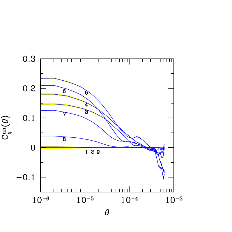
Figure 3: Evolution of the ionization autocorrelation function $C_{\chi}^{nn}(\theta)$ with $n=1,..,9$, where $n$ labels the redshift as explained in the text. Also shown are the statistical errors (shaded areas).

In Fig.3 we show the autocorrelation functions $C_{\chi}^{nn}$ along with the corresponding errors; the largest error in the curves is $1.9$% The behavior of $C_{\chi}$ is rather flat for small angles ($\theta\lower 2.15277pt\hbox{$\;\buildrel<\over{\sim}\;$}10^{-5}$ rad) and decreases rapidly for larger separations; for even larger values of $\theta$, $C_{\chi}$ becomes negative, implying that the ionization regions are anticorrelated. The position of the first zero, $\theta_{0}$, provides an estimate of the typical size of the ionized regions (including overlapping) at the corresponding redshift through the relation $R\simeq 0.23(\theta_{0}/10^{-4}{\rm rad})h^{-1}$ Mpc. The amplitude of the anticorrelation signal is roughly proportional to the correlation one. For small separations $C_{\chi}^{nm}$ can be approximated by a modified Lorentzian function of the type

$$\frac{A_{max}}{1\;+\;[(\theta-\theta_{min})/\Gamma]^{\alpha}}\;,$$ (10)

where $A_{max}$ is the maximum amplitude at $\theta=\theta_{min}$, and $\Gamma$ is the width, $\alpha$ is the power index. The values of these fitting parameters for the autocorrelation functions are given in Tab. 1.

The anticorrelated regions cannot be described in terms of such a simple assumption. Therefore the shape is different from the Gaussian one proposed by Gruzinov & Hu 1998) with redshift-dependent amplitude and standard deviation. The autocorrelation functions for any $n$ are always larger than those obtained by correlating slices at different redshifts ($m\neq n$), although the shape remains similar. We have also checked that the results do not depend on the particular slice used provided it is located not too far from the center of the simulation box. Off-center planes might lead to sensibly different amplitudes of ${\cal C}_{\chi}$ ($\approx\pm 20$%) due to border effects, only if their position is closer than $0.04L$ to the box walls.

5 RESULTS AND CONCLUSIONS

By using the derived ionization correlation function, we can calculate the angular power spectrum produced by the inhomogeneous part of the reionization from eq. 2. In Fig. 4 we show the behavior of the two-point correlation function, $C(\theta)$, and of the angular power spectrum $C_{\ell}$ which, for $\ell\gg 1$, can be approximated by

$$C_{\ell}=2\pi\int_{0}^{\infty}d\theta\theta J_{0}(\ell\theta)C(\theta).$$

The correlation function smoothly decreases from its maximum $C(0)\approx 5\times 10^{-12}$ and becomes negative at $\theta=1.7\times 10^{-4}$ rad as a result of the anticorrelation discussed above. Beyond the second null point ($\theta\approx 5\times 10^{-4}$ rad) it rapidly becomes more noisy due the decreasing number of data points in the simulation at these large separations. In addition to the statistical error, this region is also affected by systematic errors. These are mainly due to the finite size of the box which does not allow to take into account ionized regions produced by sources located just outside the simulation volume.

To minimize the of this effect we have cut the spectrum beyond separations that are larger than the minimum difference between the angular size of the box and the typical angular size of the ionized regions $\theta_{0}$ (see previous Section). This procedure should yield a $C(\theta)$ reliably unaffected by systematic errors below $\theta_{c}\approx 6\times 10^{-4}$ rad: we therefore limit our analysis to the angular interval $\theta_{min}<\theta<\theta_{c}$.

The reported angular power spectrum therefore extends in the range $5000\lower 2.15277pt\hbox{$\;\buildrel<\over{\sim}\;$}\ell\lower 2.15277pt\hbox{$\;\buildrel<\over{\sim}\;$}10^{6}$ because of the relation $\ell=\pi/\theta$. The spectrum shows an absolute maximum around $\ell\approx 30000$, where it has the value $2\times 10^{-12}$. Beyond $\ell\approx 10^{5}$ ringings appear in Fig. 4 which are caused by the abrupt cutoff of $C(\theta)$ at $\theta_{c}$, but up to $\ell\approx 10^{5}$ the behaviour of angular spectrum is not very far from flatness. We have calculated a running average $S_{\ell}$ of the spectrum (also shown in Fig. 4) through the formula

$$S_{\ell}={1\over 2\pi}\sum_{\lambda=\ell/2}^{3\ell/2}\lambda C_{\lambda},$$ (11)

This allows to get rid of the ringings (which have essentially zero average) and to appreciate the decrease to zero of the spectum above $\ell=2\times 10^{5}$. Our results match very closely those obtained by Knox et al.  (1998). In particular, the best agreement is found with their correlated-source model corresponding to $z_{i}=35,\delta z=4$. On the other hand, our numerically derived values are $z_{i}\approx 30,\delta z\approx 15$ (also notice that our evolution of $\bar{\chi}(z)$ is nonlinear). Therefore the close agreement can be regarded as rather accidental, given also the various assumptions made in that work; we recall that we have derived here the spatial distribution and evolution of the ionization fraction from numerical simulations in which several feedback effects regulating the formation of the ionizing sources have been included. Also shown for comparison in Fig. 4 are the primary angular spectra corresponding to a CDM model with the same parameters adopted here, in which the effects of a homogeneous reionization with total $\tau=0.177$ (as derived from our simulations) are either neglected or includuded. These spectra have been obtained by running CMBFAST (Seljak & Zaldarriaga 1996). The maximum value of our angular spectrum is comparable to, but higher than the most recent estimates of the Vishniac signal (Jaffe & Kamionkowski 1998, Hu 1999). For a cluster-normalized CDM model (which is thereby directly comparable with ours), Jaffe & Kamionkowski (1998) find a peak signal $\approx 8\times 10^{-13}$, which is however located at lower multipole numbers, around $\ell\approx 5000$. We also note that our predicted maximum value is typically smaller than the peak anisotropy in un uncorrelated-source models with large ionized bubbles. For instance it is about 3 times smaller than the estimate given by Gruzinov & Hu (1998), for their favorite model with $z_{i}=30,\delta z=5,R=3$ Mpc [the difference is smaller if we consider more refined computation of Knox et al (1999)]. For such uncorrelated-source models however a large bubble size implies that the peak is confined to $\ell\lower 2.15277pt\hbox{$\;\buildrel<\over{\sim}\;$}5000$. In any case, all of these models predict that the signal from IHR should dominate both the primary and the Vishniac one for $\ell\lower 2.15277pt\hbox{$\;\buildrel>\over{\sim}\;$}5000$.

The detection of this signal would be of great importance for the study of early galaxy formation, the IGM and the nature of the reionization sources. If reionization is predominantly produced by stellar type objects, as assumed here, the relatively small, sub-Mpc sizes of the ionized patches and their correlation properties, tend to shift the peak of the power spectrum towards larger multipole values, $\ell\approx 30000$. This detection will require the use of the next generation of millimiter wavelength interferometers like ALMA .This instrument is expected to reach sensitivities of 2 $\mu$K in one hour and reach $\ell\approx 10^{6}$, thus appearing as a perfect instrument to search for signatures of IHR, and, in general, for the above type of studies. Coupled with theoretical predictions for different cosmological models and simulations exploring a wide range of variation of the key parameters, as $f_{b\star}$ and $f_{esc}$, these experiments can give a comprehensive and clean view of how reionization proceeded in the universe.

Instruments nearer in the future as MAP and PLANCK could at least clarify and constrain the role, if any, played by quasars in the reionization process. Mini-quasars have been advocated by some authors (Haiman, Madau & Loeb 1999) as possible sources for reionization; in this scenario, we would expect larger patch sizes and a spectrum peaked at lower values of $\ell$, as in the uncorrelated-source models with $R$ of order a few Mpc. However, uncertainties might remain related to the duty-cycle of such objects, if they exist.

IHR might in principle affect the determination of cosmological parameters planned with future experiments. Our calculations do not allow us to quantify the uncertainty introduced because the finite size of the simulation box prevents extension of our results below $\ell\approx 5000$, where the primary spectrum should be already more than one order of magnitude smaller as shown by Fig. 4. However, since from our results the angular spectrum appears to be already declining for decreasing $l$ for $l<10^{4}$, a comparison with the results of Knox et al.  (1998) seems to imply that the impact of IHR on PLANCK may somewhat less than in their analytical model. Those authors also conclude that the very small scales affected by IHR do not sensibly alter the parameter determination obtained by MAP; our results further support their conclusion.

Although our calculations do not include the polarization angular spectrum $C_{P\ell}$, a rough estimate can be obtained extrapolating the analytic results of Hu (1999) to the present case. According to this author $C_{P\ell}/C_{\ell}\approx 10^{-1}(Q_{rms}/v_{rms})^{2}$, where the ratio of rms quadrupole to rms velocity field is evaluated at $z=z_{i}$ assuming $\delta z/z_{i}\ll 1$. Although the simulations show that $\delta z/z_{i}\approx 1$, we can nevertheless infer that $C_{P\ell}/C_{\ell}\approx 10^{-5}$. Since for $\tau=0.177$ the “linear” angular spectrum has $C_{P\ell}/C_{\ell}\approx 10^{-2}$ for large $\ell$, we conclude that the impact of IHR on cosmological parameter determination by PLANCK will be even less when polarization data are taken into account. The joint exploitation of temperature and polarization power spectra (Efstathiou & Bond 1998, Kinney 1998) is in fact required for the removal of some cosmological parameter degeneracies.

We would like to thank R. Scoccimarro for useful suggestions and P. de Bernardis, S. Masi, and V. Natale for stimulating discussions. This work is partly supported by a MURST-COFIN98 (AF) and Agenzia Spaziale Italiana-ASI (RF) grants.

$C^{mn}_{\chi}$	$z$	$A_{max}$	${\Gamma}$	$\alpha$
$C^{33}_{\chi}$	14.3	0.147	$3.8\times 10^{-5}$	1.6
$C^{44}_{\chi}$	15.4	0.180	$3.7\times 10^{-5}$	1.2
$C^{55}_{\chi}$	16.5	0.234	$3.0\times 10^{-5}$	1.4
$C^{66}_{\chi}$	18.0	0.209	$2.4\times 10^{-5}$	1.5
$C^{77}_{\chi}$	19.8	0.125	$2.1\times 10^{-5}$	1.6
$C^{88}_{\chi}$	22.1	0.039	$1.7\times 10^{-5}$	1.7

Table 1: Autocorrelation function fitting parameters

Figure available at http://www.arcetri.astro.it/$\sim$ferrara/reion.html

Figure 1: Snapshot of the distribution of ionized regions in the simulation box at redshift $z=19.8$ for run A

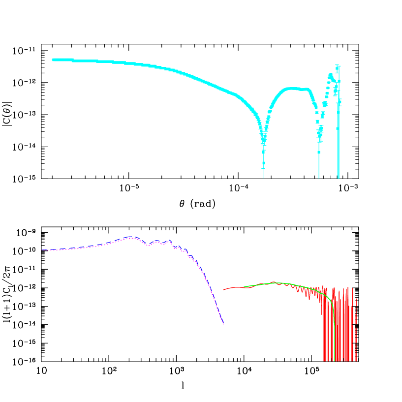
Figure 4: Top: Angular correlation function $C(\theta)$; Bottom: Power spectrum $C_{\ell}$ of secondary anisotropies produced by IHR; superposed is the running spectrum average $S_{\ell}$. The curves on the left are the primary spectra in which homogenous reionization effects are neglected (solid) or included (dashed) with a reionization optical depth $\tau=0.177$.

References

- (1) Aghanim, N., Desert, F. X., Puget, J. L. & Gispert, R. 1996, A&A, 311, 1
- (2) Aghanim, N., Desert, F. X., Puget, J. L. & Gispert, R. 1999, A&A, 341, 640
- (3) Ciardi, B., Ferrara, A. & Abel, T. 1999, ApJ, in press (astro-ph/9811137)
- (4) Ciardi, B., Ferrara, A., Governato, F. & Jenkins, A. 1999, preprint (astro-ph/9907189,CFGJ)
- (5) De Bernardis, P., Balbi, A., De Gasperis, G., Melchiorri, A. & Vittorio, N. 1997, ApJ, 480, 1
- (6) Efstathiou, G. & Bond, J.R. 1998, MNRAS, 304, 75
- (7) Efstathiou, G., Bond, J.R. & White, S.D.M. 1992, MNRAS, 258, 1P
- (8) Gnedin, N. Y. 1998, MNRAS, 294, 407.
- (9) Gnedin, N. Y. 1999, preprint (astro-ph/9909383)
- (10) Griffiths, L. M., Barbosa, D. & Liddle, A.R. 1999, MNRAS, in press (astro-ph/9812125)
- (11) Groth, , E. J., Juskiewicz, R. & Ostriker, J. P. 1989, ApJ, 346, 558
- (12) Gruzinov, A. & Hu, W. 1998, ApJ, 508, 435.
- (13) Haiman, Z., Madau, P. & Loeb, A. 1999, preprint (astro-ph/9805258).
- (14) Haiman, Z. & Knox, L. 1999, preprint (astro-ph/9902311)
- (15) Hu, W. 1999, preprint (astro-ph/9907103)
- (16) Jaffe, A. H. & Kamionkowski, M. 1999, preprint (astro-ph/9801022 v3)
- (17) Kinney, W.H. 1998, Phys. Rev. D 58, 123506
- (18) Knox, L., Scoccimarro, R. & Dodelson, S. 1998, Phys. Rev. Lett., 81, 2004
- (19) Oh, S. P. 1998, preprint (astro-ph/9812318).
- (20) Peebles, P. J. E. & Juszkiewicz, R. 1998, ApJ, 509, 483
- (21) Seljak, U. & Zaldarriaga, M. 1996, ApJ, 469, 437
- (22) Steidel, C. C. et al. 1998, preprint (astro-ph/9811399)
- (23)