The precession of eccentric discs in close binaries

Abstract

We consider the precession rates of eccentric discs in close binaries, and compare theoretical predictions with the results of numerical disc simulations and with observed superhump periods. A simple dynamical model for precession is found to be inadequate. For mass ratios $\ \raisebox{-1.29167pt}{$\stackrel{{\scriptstyle<}}{{\scriptstyle\sim}}$}\ 1/4$ a linear dynamical model does provide an upper limit for disc precession rates. Theory suggests that pressure forces have a significant retrograde impact upon the precession rate (Lubow 1992). We find that the disc precession rates for three systems with accurately known mass ratios are significantly slower than predicted by the dynamical theory, and we attribute the difference to pressure forces. By assuming that pressure forces of similar magnitude occur in all superhumping systems, we obtain an improved fit to superhump observations.

1 Introduction

Superhumps are now commonly found in short period cataclysmic variables (Patterson 1998) and X-ray binaries (O’Donoghue & Charles 1996). The most likely explanation is that these periodic luminosity variations are caused by the tidal stresses on an eccentric, precessing accretion disc (Whitehurst 1988; Hirose & Osaki 1990; Lubow 1991). In this model, the superhump period, $P_{\rm sh}$, equates to the period of the disc’s precession, $P_{\rm d}$, as measured in the binary frame. Although reliable measurements of $P_{\rm sh}$ have been made for at least 53 separate systems (Patterson 1998), the observations have yet to be compared properly with the model’s theoretical predictions.

In this paper we consider the factors determining the precession rate of an eccentric disc, and compare our theoretical understanding, simulation results and the observations.

2 disc precession periods

It is now well established that in binaries with mass ratios $q\ \raisebox{-1.29167pt}{$\stackrel{{\scriptstyle<}}{{\scriptstyle\sim}}$}\ 1/4$ it is possible for eccentricity to be excited in the accretion disc at the $3:1$ eccentric inner Lindblad resonance (Lubow 1991). Here we define $q=m_{\rm 2}/m_{\rm 1}$ to be the mass of the donor star divided by the mass of the accreting star. Under certain circumstances, eccentricity may be excited in systems with mass ratios as large as $1/3$ (Murray, Warner & Wickramasinghe 1999).

How an eccentric disc precesses coherently has been a source of confusion. For a single particle, the rate at which an elliptical orbit precesses

$$\omega_{\rm dyn}=\Omega-\kappa.$$ (1)

Now, for a given gravitational potential, a particle’s angular frequency, $\Omega$, and radial or epicyclic frequency, $\kappa$, are both functions of $r$. Hence the precession rate, $\omega$, also depends upon the mean radius of the orbit. Yet neither the observations (Patterson 1998) nor the simulations (Murray 1998) yield any indication of differential precession. So how does a disc, that extends over a range of radii, organize itself to precess with a unique frequency?

The answer is that we are not dealing with a collection of isolated test particles, but with a gaseous disc. The eccentricity is excited at the Lindblad resonance, and then propagates inwards through the disc as a wave, getting wrapped into a spiral by the differential rotation of the gas (Lubow 1992). If the spiral is wound up on a length scale much smaller than the radius (the tight winding limit), then $\omega$, the rate of azimuthal advance of the eccentricity, is governed by the dispersion relation

$$(\Omega-\omega)^{2}=\kappa^{2}+k^{2}c^{2},$$ (2)

where $c$ is the sound speed of the gas, and $k$ is the radial wavenumber of the spiral (see e.g. Binney & Tremaine 1987). Now, as $\omega$ is much less than $\Omega$ and $\kappa$ we have

$$\omega \simeq \Omega-\kappa-k^{2}c^{2}/(2\Omega)$$ (3)

$$= \omega_{\rm dyn}-k^{2}c^{2}/(2\Omega).$$ (4)

$\omega$ is determined for the wave in the region in which it is launched. As the wave propagates inwards, the frequency remains constant but the wavelength changes in response to the changing environment through which it moves.

The above arguments are based upon the analysis of Lubow (1992). He also identified a third factor that contributed to the precession when the magnitude of the eccentricity was changing secularly. In this paper we are interested in the long term mean value for $\omega$ and so this extra term need not be considered further.

Equation 4 tells us that a gaseous disc will precess more slowly than a ballistic particle at the resonance radius. Lubow (1992) estimated that pressure effects could reduce $\omega$ by approximately one percent of $\Omega$. Now $\omega_{\rm dyn}$ is itself of the order of a few per cent of $\Omega$, so the reduction is significant. (Simpson & Wood (1998) misinterpreted Lubow’s work and ignored the pressure term as being a few percent of the dynamical precession).

Hirose & Osaki (1993) obtained estimates for the superhump period by solving the eigenvalue problem of a linear one-armed mode in an inviscid disc. Their arguments correspond with those given above and their results agree very well with those of Lubow (1992). They showed that an increase in disc temperature allowed the eccentric mode to propagate further into the disc, with the precession rate being reduced as a result. Lubow (1992) also completed several two dimensional hydrodynamic disc simulations, in which he isolated the various contributing factors to the precession. His numerical results clearly showed pressure forces to be important. In fact, for those particular simulations, the pressure contributions reduced $\omega$ to half the dynamical value. Till now, observational data has only been compared with dynamical estimates for the precession that we know to be inadequate.

3 The theory and simulations compared

The numerical simulations of Whitehurst (1988) lead directly to the eccentric disc model for superhumps. In this section we compare subsequent numerical results (Hirose & Osaki 1990; Kunze, Speith & Riffert 1997; Murray 1998; Simpson & Wood 1998; Murray et al. 1999) with the dynamical equation for precession (equation 1). We do not attempt a comparison with the hydrodynamic equation as the simulations of Hirose & Osaki were completed using the sticky particle method due to Lin & Pringle (1976) which does not account for pressure forces.

For approximately circular orbits, the rate of dynamical precession

$$\omega_{\rm dyn}=a(r)\,\frac{q}{\sqrt{1+q}}\,\Omega_{\rm orb},$$ (5)

where

$$a(r)=\frac{1}{4\,r^{1/2}}\,\frac{d}{dr}(r^{2}\,\frac{db^{(0)}_{1/2}}{dr}).$$ (6)

$b^{(j)}_{s}$ is the standard notation for a Laplace coefficient from celestial mechanics. We have made use of the hyper-geometric series expression for $b^{(j)}_{s}$ found in Brouwer & Clemence (1961) (equation 42, Chapter 15) to evaluate $a(r)$ as a function of radius (see figure 1). Clearly, the precession rate of a ballistic particle is an increasing function of radius. But as mentioned above, differential precession is not observed. Thus in previous applications of the dynamical theory to discs, it was assumed that the entire disc precessed as if it were a single ballistic particle at the resonance radius, $r_{\rm res}\simeq 0.477\,$$d$, (see e.g. Hirose & Osaki). Unfortunately, most of these comparisons are of little value because they either failed to correctly evaluate $a(r)$ (e.g. Patterson 1998) or they made use of an incorrect equation for the precession that first appeared in Whitehurst & King (1991).

Figure 1: $a(r)$ is the term encapsulating the radial dependence of the dynamical precession rate. Calculated using the hyper-geometric series (Brouwer & Clemence, 1961).

Observational data is usually presented in terms of the superhump period excess

$$\epsilon=\frac{P_{\rm sh}-P_{\rm orb}}{P_{\rm orb}}.$$ (7)

In terms of the disc precession rate $\omega$,

$$\epsilon=\frac{\omega}{\Omega_{\rm orb}-\omega}.$$ (8)

So in figure 2 we have plotted as a function of mass ratio the superhump period excesses obtained from the disc simulations of several different authors. The solid curve shows the superhump period excess estimated by equation 5 with $r=r_{\rm res}$.

Figure 2: Collation of superhump period excesses from; Murray (1998), Murray et al. (1999) and this paper (filled circles), Hirose & Osaki (triangles), Simpson & Wood (asterisks), and Kunze et al. (hollow squares). The solid curve is the dynamical contribution to the period excess at the resonance radius (as calculated using equation 5) from this paper, Simpson & Wood, and Kunze et al. lie very close to one another on this plot.

All authors used the smooth particle hydrodynamics (SPH) technique, except Hirose & Osaki who used the sticky particle technique. The pressure contribution to the disc precession is thus absent from their simulations. The various implementations of SPH are described in Flebbe et al. (1994), Simpson & Wood (1998), and Murray (1996).

The calculations completed for Murray (1998), and Murray et al. (1999) were of very cool isothermal discs. In units of the binary separation, $d$, and the orbital angular frequency, $\Omega_{\rm orb}^{-1}$, we set the sound speed $c=0.02\,$$d\,\Omega_{\rm orb}$. The pressure contribution is proportional to the square of the sound speed and so was very small. We also used a very large value for the shear viscosity. This reduced the viscous time scale to a value that enabled us to follow the evolution of discs to steady state in a reasonable amount of computing time. However with a larger shear viscosity it was easier for material to penetrate the resonance. Significantly eccentric discs and very strong superhump signals were obtained as a result. Furthermore, the large shear viscosity inhibited the inward propagation of the eccentricity and further reduced the effectiveness of the pressure term in equation 4.

Without the benefit of any significant pressure contribution to the disc precession, the points from Murray (1998) and Hirose & Osaki lie very close to the dynamical precession curve. Some are marginally above the curve. As mentioned above, the large shear viscosities used allowed the discs to effectively penetrate the resonance and extend to somewhat larger radii. On the other hand the four points from Murray et al. (1999) are all well above the curve, and cannot be explained in terms of large discs. For these mass ratios the resonance lies beyond the tidal truncation radius. That is, for $q\ \raisebox{-1.29167pt}{$\stackrel{{\scriptstyle>}}{{\scriptstyle\sim}}$}\ 1/4$ simply periodic orbits begin intersecting one another inside $r_{\rm res}$. The orbits in this region will no longer be approximately circular, in contradiction of the assumption underlying the analytical expressions in Hirose & Osaki, and Lubow (1992). We conclude therefore that, gas pressure considerations aside, expressions such as equation 5 will only be valid for mass ratios less than approximately 1/4.

The discs of Simpson & Wood, and of Kunze et al. precessed significantly more slowly than expected from purely dynamical considerations (these points lie below the dynamical curve in figure 2). Kunze et al. assumed each element of the disc radiated as a blackbody and set the sound speed according to the blackbody temperature. Simpson & Wood used a polytropic equation of state with index $\gamma=1.01$ and integrated the internal energy equation for each particle. Although a comparison is not straightforward, these discs would have been somewhat hotter than the ones constructed for this paper. As a consequence, the retrograde contribution to the precession due to pressure forces would have been larger, and the values for $P_{\rm d}$ obtained by Simpson & Wood and Kunze et al. are closer to observed $P_{\rm sh}$.

We are currently running a set of simulations with the shear viscosity ten times smaller than in Murray (1998), but with other parameters unchanged. In particular, the sound speed $c=0.02\,$$d\,\Omega_{\rm orb}$. This gives an effective value of the Shakura-Sunyaev parameter $\alpha\simeq 0.16$ at the resonance (as opposed to $\simeq 1.6$ in the previous calculations). At present we have results only for $q=0.10$ (the simulations now take much longer to complete). This particular calculation ran for 100 orbital periods. As is to be expected, the superhump amplitude was reduced. At the conclusion of the calculation the superhump period (averaging over 25 superhump cycles) $P_{\rm sh}=(1.0295\pm 0.0005)\,P_{\rm orb}$. This period is significantly below the dynamical precession curve even though the disc is very cool, and it corresponds very well with the results of Simpson & Wood, and Kunze et al. Our result has been included in figure 2 but we emphasize that at the conclusion of the simulation, the disc mass was still very slowly increasing, and the superhump period had not completely stabilised.

In the above discussion we did not refer to the calculations of Whitehurst (1994) simply because he used an initial mass transfer burst to set up his discs, and the superhump periods were not obviously steady state values. The simulations described in section 4.2 illustrate the time scale upon which resonant discs adjust to changes in the mass transfer rate. Before we leave this subject, a word of warning. We discovered in one particular trial simulation that once mass return from the outer edge of the disc to the secondary star occurred, the superhump period excess was reduced by approximately $5\,\%$. The explanation is simple. Material at the outer edge of the disc precesses most rapidly. Remove that material and you slow the disc precession. This effect can hinder comparison with theory and other simulations. Such mass return occurred in the simulations of Hirose & Osaki and of Simpson & Wood.

We conclude that for mass ratios less than $1/4$, equation 5 provides a useful upper limit for the steady state precession rate of a gaseous disc. However, for systems with $q\ \raisebox{-1.29167pt}{$\stackrel{{\scriptstyle>}}{{\scriptstyle\sim}}$}\ 1/4$, the intersection of simply periodic orbits near the resonance radius renders equation 5 invalid.

The next step is to compare simulation results with eigenmode calculations such as those performed by Hirose & Osaki (1993). They tabulated disc precession rates as a function of the sound speed at the resonance for systems with mass ratios $q=0.15$ and $0.05$. Both the eigenmode calculations and the hydrodynamic simulations show similar magnitude pressure contributions to the precession. However, as yet the assumptions made in making the two sets of calculations (e.g. equation of state) differ sufficiently as to prevent a more detailed comparison.

4 Theory and observation compared

Patterson (1998) tabulated the superhump period excesses for 53 systems. In this section we will compare this data with both the dynamical and hydrodynamical equations for precession. In order to do this we require an independent means of estimating a system’s mass ratio. Unfortunately, although the mass of the secondary star as a function of orbital period is reasonably well constrained, there is evidence of considerable variation in the white dwarf masses of otherwise similar systems (see e.g. Smith & Dhillon 1998, figure 5). The resulting uncertainty in $q$ is large enough to interfere with our comparisons with theory. An early attempt to compare theory and observation by Molnar & Kobulnicky (1992), was hampered in exactly this fashion (see their figure 2).

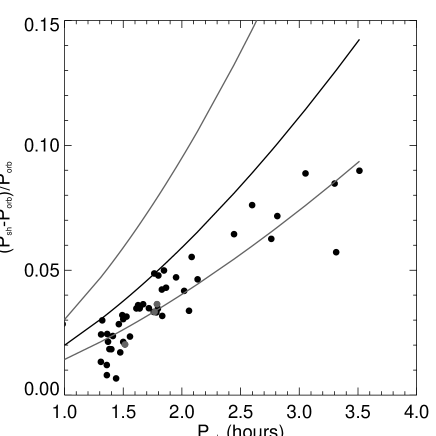
Figure 3: Observed superhump period excesses (data from Patterson, 1998) plotted against orbital period. Overlaid are curves for the dynamical precession as calculated using equation 5, and assuming a white dwarf mass $M_{\rm wd}=0.76\pm 0.22\,M_{\odot}$, and the secondary mass period relationship from Smith & Dhillon (1999), i.e. $M_{\rm sec}/M_{\odot}=(0.038\pm 0.003)P^{(1.58\pm 0.09)}$. The outlying curves incorporate the uncertainties in the Smith & Dhillon values.

In figure 3 we have plotted the superhump data from Patterson (1998) against theoretical predictions for the dynamical precession (made using equation 5 with $r=r_{\rm res}$). In order to estimate the mass ratio of a system of given orbital period we have used the observationally derived stellar masses obtained by Smith & Dhillon (1998). They found the mean white dwarf mass for all cataclysmic variables to be $0.76\pm 0.22\,M_{\odot}$, and they estimated that $M_{\rm sec}/M_{\odot}=(0.038\pm 0.003)P^{(1.58\pm 0.09)}$. The central (darker) curve in figure 3 represents the best theoretical estimate. The outer two curves show the consequences of the uncertainty in the Smith & Dhillon values for the theory. In fact, Smith & Dhillon found the mean white dwarf mass for systems below the period gap to be $0.69\pm 0.13\,M_{\odot}$, and to be $0.80\pm 0.22\,M_{\odot}$ for systems above the period gap. However precession rates recalculated using the adjusted white dwarf masses differed only marginally from the original estimates.

Assumptions about stellar masses aside, figure 3 shows that the superhump observations cannot be adequately explained in terms of simple dynamical precession. The retrograde precession due to pressure forces is necessary to bring closer agreement between theory and observations. Previously published figures showing closer agreement between dynamical precession estimates and observations only did so because the dynamical precession was calculated incorrectly. For example Patterson (1998) used the equation

$$\omega_{\rm dyn}/\Omega_{\rm orb}=0.23\,\frac{q}{\sqrt{1+q}}.$$ (9)

The coefficient should be approximately $0.4$ (see Hirose & Osaki 1990; Lubow 1992; figure 1 above). In order to explain superhumps in long period systems with equation 9, mass ratios as high as $0.5$ are required. These $q$ values are clearly incompatible with eccentricity excitation at the $3:1$ inner Lindblad resonance. However, if we use the more defensible equation 4 for the precession, then smaller mass ratios are obtained.

Our confidence in the comparison between theory and observation is limited by uncertainty in $q$. The inadequacy of the dynamical expression for precession is much more clearly apparent when we consider the eclipsing systems OY Car, HT Cas and Z Cha. Very accurate determinations of the mass ratios of these systems are respectively obtained in Wood et al. (1989), Horne, Wood & Stiening (1991), and Wood et al. (1986). In Table 1 we list for each system the observed $\omega$ and the dynamical precession rate. In each case the difference between the two values is too large to be explained by uncertainties in either $q$ or equation 5. The difference is simply the (retrograde) pressure contribution to the precession.

We can check whether the inferred $\omega_{\rm pr}$ is consistent with the assumption that the eccentricity is tightly wound. The pitch angle $i$ of the spiral wave is given by $\cot i=|kr|$. Thus, substituting for $k$ in equation 4, we find that the pressure contribution to the precession rate at the $3:1$ resonance

$$\omega_{\rm pr}\simeq-\frac{2}{3}\,\Omega_{\rm orb}\,(\frac{c}{\Omega_{\rm orb}\,d\,}\frac{1}{\tan{i}})^{2}.$$ (10)

Note that Lubow (1992) had the constant of proportionality inverted in his equation 21. If we assume the sound speed at the resonance radius $c=0.05\,d\,\Omega_{\rm orb}$ then we obtain pitch angles of $17,16$ and $15^{\circ}$ for OY Car, Z Cha and HT Cas respectively. These are certainly consistent with the tight winding approximation.

We complete this section with a comparison of the observations with the predictions of the hydrodynamic theory. As it is not clear what value $k$ should take in equation 4, we make the naive assumption that the pressure contribution to precession in all 53 systems tabulated in Patterson (1998) will be similar to that of OY Car, HT Cas and Z Cha. We take a mean value for $\omega_{\rm pr}=-1.9\,{\rm rad}\,{\rm day}^{-1}$, and plot predicted precession rates against the observations in figure 4. A much improved fit is achieved. As with figure 3, three curves are drawn to show the influence of uncertainty in our knowledge of white dwarf and secondary masses. Much of the difference between the curves is due to the uncertainty in white dwarf mass, with the uppermost curve corresponding to $M_{\rm wd}=0.54\,M_{\odot}$. The observational data is perhaps best fit with a curve generated assuming a white dwarf mass $\simeq 0.65\,M_{\odot}$.

We recall that equation 5 underestimates the dynamical precession rate for systems with mass ratios $\ \raisebox{-1.29167pt}{$\stackrel{{\scriptstyle>}}{{\scriptstyle\sim}}$}\ 1/4$. Thus the theoretical curves should rise more steeply long-wards of say $P_{\rm orb}=3$ hr. The implication then is that long period superhumpers have significantly more massive white dwarfs than do their shorter period counterparts. As a consequence the mass ratios of the long period systems will be smaller than previously estimated. This is qualitatively consistent with the eccentricity being excited at the $3:1$ Lindblad resonance, and with our previous result (Murray et al. 1999) that the excitation can occur at mass ratios $\ \raisebox{-1.29167pt}{$\stackrel{{\scriptstyle<}}{{\scriptstyle\sim}}$}\ 1/3$. In other words, of those systems with say $P_{\rm orb}\simeq 3$ hrs, only those with more massive white dwarfs will exhibit superhumps. This then is distinct from any effect caused by systematic variation in white dwarf masses in the cataclysmic variable population as a whole.

Table 1: The observed disc precession rate (in rad ${\rm day}^{-1}$) for three systems with accurately known mass ratios. The dynamical precession rate is calculated using equation 5 The pressure contribution is then simply the difference between those two values.

System	$q$	$\omega_{\rm obs}$	$\omega_{\rm dyn}$	$\omega_{\rm pr}$
OY Car	$0.102\pm 0.003$	1.977	3.869	-1.892
Z Cha	$0.15\pm 0.03$	2.961	4.712	-1.751
HT Cas	$0.15\pm 0.03$	2.75	4.773	-2.02

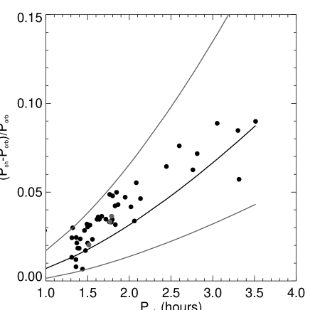
Figure 4: Observed superhump period excesses (data from Patterson, 1998) plotted against orbital period. Overlaid are curves for the hydrodynamic precession as calculated using equation 4, with $\omega_{\rm pr}=-1.9{\rm rad}\,{\rm day}^{-1}$. We assume a white dwarf mass $M_{\rm wd}=0.76\pm 0.22\,M_{\odot}$, and the secondary mass period relationship from Smith & Dhillon (1999), i.e. $M_{\rm sec}/M_{\odot}=(0.038\pm 0.003)P^{(1.58\pm 0.09)}$. The outlying curves incorporate the uncertainties in the Smith & Dhillon relation.

5 Conclusions

We have compared the theoretical predictions for the precession rates of eccentric discs with simulation results and with observed superhump periods. Comparison with disc simulations showed that the dynamical equation provided a useful upper limit for the disc precession rate of systems with mass ratios $\ \raisebox{-1.29167pt}{$\stackrel{{\scriptstyle<}}{{\scriptstyle\sim}}$}\ 1/4$.

Previous papers showing good agreement between observations and a simple dynamical model for precession are based on incorrectly calculated dynamical expressions. The consequence of using these models is that very large mass ratios are predicted for the long period superhumpers. At such large mass ratios the resonance lies well beyond the truncation radius of the disc and eccentricity cannot be excited.

We show that when the correct expression for dynamical precession is used, there is poor agreement with the observations. This can be seen even though there is considerable uncertainty in estimating the mass ratio of a system of given orbital period.

The observed superhump periods of the eclipsing systems OY Car, Z Cha and HT Cas are shown to be significantly less than predicted by the dynamical theory, demonstrating that the retrograde contribution of pressure forces is important.

The inclusion of a retrograde pressure contribution to the precession rate not only improves the fit to the data but also requires long period superhumpers have smaller mass ratios than previously thought. This in turn is more consistent with the eccentricity being generated at the $3:1$ Lindblad resonance.

References

- [1] Binney, Tremaine, 1987, Galactic Dynamics, Princeton University Press, Princeton, New Jersey
- [2] Brouwer, D., Clemence, G.D., 1961, Methods of Celestial Mechanics, Academic Press, London
- [3] Flebbe, O., Muenzel, S., Herold, H.; Riffert, H., Ruder, H., 1994, ApJ, 431, 754
- [4] Hirose, M., Osaki, Y., 1990, PASJ, 42, 135
- [5] Hirose, M., Osaki, Y., 1993, PASJ, 45, 595
- [6] Horne, K., Wood, J.H., Stiening, R.F., 1991, ApJ, 378, 271
- [7] Kunze, S., Speith, R., Riffert, H., 1997, MNRAS, 289, 889
- [8] Lin, D.N.C., Pringle, J.E., 1976, in Eggleton, P., Structure and Evolution of Close Binary Systems, Reidel, Dordrecht
- [9] Lubow, S.H., 1991, ApJ, 381, 259
- [10] Lubow, S.H., 1992, ApJ, 401, 317
- [11] Molnar, L.A., Kobulnicky, H.A., 1992, ApJ, 392, 678
- [12] Murray, J.R., 1996, MNRAS, 279, 402
- [13] Murray, J.R., 1998, MNRAS, 297, 323
- [14] Murray, J.R., Warner, B., Wickramasinghe, D.T., 1999, MNRAS, submitted
- [15] O’Donoghue, D., Charles, P.A., 1996, MNRAS, 282, 191
- [16] Patterson, J., 1998, PASP, 110, 1132
- [17] Simpson, J.C., Wood, M.A., 1998, ApJ, 506, 360
- [18] Smith, D.A., Dhillon, V.S., 1999, MNRAS, in press
- [19] Whitehurst, R., 1988, MNRAS, 232, 35
- [20] Whitehurst, R., 1994, MNRAS, 266, 35
- [21] Whitehurst, R., King, A.R., 1991, MNRAS, 249, 25
- [22] Wood, J.H., Horne, K., Berriman, G., Wade, R.A., 1989, ApJ, 341, 974
- [23] Wood, J.H., Horne, K., Berriman, G., Wade, R.A., O’Donoghue, D., Warner, B., 1986, MNRAS, 219, 629