Magnetic Fields in Quasar Cores II

Abstract

Multi-frequency polarimetry with the Very Long Baseline Array (VLBA) telescope has revealed absolute Faraday Rotation Measures (RMs) in excess of 1000 rad m^-2 in the central regions of 7 out of 8 strong quasars studied (e.g., 3C 273, 3C 279, 3C 395). Beyond a projected distance of $\sim$20 pc, however, the jets are found to have $|$RM$|$ $<$ 100 rad m^-2. Such sharp RM gradients cannot be produced by cluster or galactic-scale magnetic fields, but rather must be the result of magnetic fields organized over the central 1–100 pc. The RMs of the sources studied to date and the polarization properties of BL Lacs, quasars and galaxies are shown to be consistent so far with the predictions of unified schemes.

The direct detection of high RMs in these quasar cores can explain the low fractional core polarizations usually observed in quasars at centimeter wavelengths as the result of irregularities in the Faraday screen on scales smaller than the telescope beam. Variability in the RM of the core is reported for 3C 279 between observations taken 1.5 years apart, indicating that the Faraday screen changes on that timescale, or that the projected superluminal motion of the inner jet components samples a new location in the screen with time. Either way, these changes in the Faraday screen may explain the dramatic variability in core polarization properties displayed by quasars.

1 Introduction

At sufficiently high angular resolution ($\sim$1 mas), the inner jets of some quasars have been found to exhibit Faraday Rotation Measures in excess of 1000 radians m^-2 (Udomprasert et al. 1997; Cotton et al. 1997; Taylor 1998). This RM is most likely produced by organized magnetic fields and ionized gas close to the center of activity. Beyond a projected distance from the core of 20 pc, the RMs in the jet fall below 100 radians m^-2 and are thus consistent with a purely galactic origin.

In §2 a sample of 40 strong, compact galaxies, quasars and BL Lacertae objects is defined. Four of these sources were reported on in Taylor 1998 (Paper I). In §3 I describe observations of four more quasars from this sample, and the results are presented in §4. In §5 the RM observations are discussed in the context of unified schemes.

I assume H${}_{0}=50$ km s^-1 Mpc^-1 and q₀=0.5 throughout.

2 Sample Selection

The sample of target sources was drawn from the 15 GHz VLBA survey of Kellermann et al.(1998). This is a sample of 132 strong, compact AGN drawn from the complete 5 GHz 1 Jansky catalogue of Kühr et al. (1981) as supplemented by Stickel, Meisenheimer & Kühr (1994). To reduce the sample size to a tractable level and facilitate scheduling, an initial flux limit of $S_{15}$ $>$ 2 Jy, where $S_{15}$ is the total 15 GHz flux measured by Kellermann et al., and declination limit of $\delta>-$10^∘ was imposed. In addition, the somewhat weaker quasars 3C 380 and 3C 395 were also observed. The final sample consists of 40 objects and is presented in Table 1. In the sample there are 25 quasars, 5 galaxies, 8 BL Lacertae objects, and 2 as yet unidentified objects. Redshifts are available for all but 3 sources.

3 Observations

3.1 Data Reduction Procedures

The observations, performed on 1998 Aug. 3 (1998.58), were carried out at multiple frequencies (or IFs) between 4.6 and 15.2 GHz (see Table 2) using the 10 element VLBA. Both right and left circular polarizations were recorded using 1 bit sampling across a bandwidth of 8 MHz. The VLBA correlator produced 16 frequency channels across each IF during every 2 second integration.

Amplitude calibration for each antenna was derived from measurements of the antenna gain and system temperatures during each run. Global fringe fitting was performed using the AIPS task FRING, an implementation of the Schwab & Cotton (1983) algorithm. The fringe fitting was performed on each IF and polarization independently using a solution interval of 2 minutes, and a point source model was assumed. Next, a short segment of the cross hand data from the strongly polarized calibrator 3C 279 (1253-055) was fringe fitted in order to determine the right-left delay difference, and the correction obtained was applied to the rest of the data. Once delay and rate solutions were applied the data were averaged in frequency. The data from all sources were edited and averaged over 20 second intervals using Difmap (Shepherd, Pearson & Taylor 1994; Shepherd 1997) and then were subsequently self-calibrated using AIPS and Difmap in combination.

Next, the strong, compact calibrator 1638+398 was used to determine the feed polarizations of the antennas using the AIPS task LPCAL. I assumed that the VLBA antennas had good quality feeds with relatively pure polarizations, which allowed me to use a linearized model to fit the feed polarizations. Once these were determined, the solutions were applied to observations of 3C 279, and to the compact source 0954+658. The polarization angle calibration of the VLBA was set using component C4 of 3C 279 which has been shown to be stable over many years (Taylor 1998). A small RM of $-$40 radians m^-2 was assumed for C4, consistent with the value of $-$64 $\pm$ 50 radians m^-2 found by Taylor (1998). The absolute electric vector position angle (EVPA) calibration is estimated to be good to about 3^∘ at all frequencies observed. This translates into an absolute uncertainty in the RM (determined by observations between 8 and 15 GHz) of 50 radians m^-2. The polarization calibration of the VLBA was verified by observing the compact source 0954+658 with the VLA on 1998 August 4. The flux density scale and polarization angle calibration at the VLA were set using 3C 286. Reasonable agreement was found between the polarized flux densities and polarization angles measured with the VLA and VLBA (see Table 3). The discrepancies are consistent with the moderately low signal-to-noise ratio of the observations of 0954+658.

4 Results

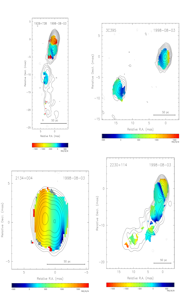
Figure 6: Rotation measure images of 1928+738, 3C 395, 2134+004, and 2230+114 with contours of total intensity superimposed. Contours are as in Figures 1, 2, 3, and 4.

In order to compare images of the total intensity, polarized intensity, and polarization angle obtained at different frequencies with a fixed array of antennas, it is necessary to taper the observations made at higher frequencies (and hence higher intrinsic resolution) in order to match the resolution of the lowest frequency observed. Various combinations of images were produced covering the ranges from 5-8 GHz, 8-15 GHz, and 12-15 GHz. The heavy taper required to match the 15 GHz to the 5 GHz resolution made this combination of limited utility. And as the cores were generally found to depolarize at 5 GHz, all of the results presented here have been derived from the 7 frequencies in the range 8–15 GHz (see Table 2). Faraday Rotation Measures were obtained by performing a least-squares fit of a $\lambda^{2}$-relation to measurements of the polarization angle at each pixel in matched-resolution images. Representative fits are shown for each source in Figures 1–5, and the RM distributions for each target sources is shown in Figure 6.

In the process of fringe-fitting the VLBA data, the brightest component of each source (in almost all cases the flat-spectrum core component) is shifted to the map center. If this core component is the location in the jet where the synchrotron self absorption optical depth is unity, then its position will vary with frequency (Blandford & Königl 1979), such that higher frequencies look “deeper” down the jet towards the true center of activity. This frequency dependent shift of the core component can be measured by using optically thin features in the jet to register simultaneous, multi-frequency observations (see e.g. Lobanov 1996). The amount of this shift is small, $<0.2$ mas between 5 and 15 GHz for 3C 345 (Lobanov 1996). For all the observations presented here, the registration of the multi-frequency observations were found to be within 10% of the beam size, and no attempt to correct for a core shift was made.

4.1 4C 73.18 (1928+738)

This relatively bright, nearby quasar ($V$ = 15.5, $z$=0.3021, 1 mas = 5.52 pc – Lawrence et al. 1996) is included in the PR sample (Pearson & Readhead 1988), and as such was imaged with VLBI in the early 1980s. These first VLBI observations were reported on by Eckart et al. (1985) who found a southward jet extending 17 mas with superluminal components moving at 0.6 mas y^-1 (14 c) relative to an assumed stationary core component. Hummel et al. (1992) monitored 1928+738 in six epochs at 22 GHz between 1985.10 and 1989.71 and found relative superluminal motions in the range 0.3 – 0.4 mas y^-1. Ros et al. (1999) were able to align three epochs taken at 5 or 8.4 GHz between 1985.77 and 1991.89 relative to the nearby BL Lac object 2007+777. Their astrometry suggests that in some epochs the core component is weak or undetected at 8.4 GHz.

Cawthorne et al. (1993) measured the linear polarization of 1928+738 at 5 GHz (epoch 1984.23) and found a fractional polarization ranging from a level of 1% at the northernmost component to 10% in the knots $\sim$10 mas to the south. At both 8 and 15 GHz (epoch 1998.59) I find 1% or less fractional polarization from the northernmost component (A) (see Fig. 1 and Table 4). The fractional polarization increases along the jet to 17% at component C, $\sim$10 mas to the south. The RM of component A is high at 2200 radians m^-2 in the rest frame of the source. However the depolarization of 0.3, indicating stronger polarization at 8.4 GHz, suggests that frequency dependent substructure is present which could influence the observed RM. In the jet the RMs fall to background levels ($-$32 $\pm$ 50) and are roughly in agreement with the RM of 33 $\pm$ 4 measured on kiloparsec scales with the VLA by Wrobel (1993).

4.2 3C 395 (1901+319)

This source was identified with a magnitude 17 quasar at $z$=0.635 (1 mas = 7.75 pc) by Gelderman & Whittle (1994). The parsec to kiloparsec scale radio structure has been reported on by Lara et al. (1997). They find a bright, unresolved core (component A) and a straight jet extending 15 mas to the east. While the inner 15 mas of the jet is straight, after that it appears to bend by 180^∘ and form a knotty jet traveling more than 500 mas in the opposite apparent direction. Given the likely orientation of the radio source close to the line-of-sight, a large intrinsic bend in the source is not required. On the arscecond scale, a halo is seen which Lara et al. interpret to to be the radio lobes seen in projection against the jet.

No VLBI polarimetric observations of 3C 395 have been previously reported. I find the core and inner jet component (marked with an A in Fig. 2) to be polarized at the $\sim$1.5% level on average, and to have an average RM of 300 radians m^-2 (see Table 4). There is a strong gradient in RM (see Figures 2 and 6), however, such that the western end reaches RMs of 1200 radians m^-2, while the eastern end is consistent with an RM of 0 radians m^-2. The western end, presumably closest to the center of activity, has just 1% polarization at 8.3 GHz. The poor fits of the RM at the western end are probably related to the low fractional polarization, and blending with the more strongly polarized eastern end. The polarization increases toward the eastern end to a maximum at the edge of 10%. The $\sim$16 mas distant component (B), is $\sim$11% polarized at 8.3 GHz and has a small RM of 68 $\pm$ 40 radians m^-2. The integrated RM measured by Simard-Normandin et al. (1981) was 169 $\pm$ 1 radians m^-2 for this moderately low galactic latitude ($b=12$^∘) source.

4.3 2134+004

This magnitude 17 quasar lies at a redshift of 1.94 (1 mas = 8.24 pc) and has been observed to vary in the optical by more than 3 magnitudes (Gottlieb & Liller 1978). Although variations in total intensity are only $\sim$15% on timescales of years (Aller, Aller & Hughes 1994), large variations were reported for the parsec-scale structure at 10.7 GHz between 1987 and 1989 requiring apparent velocities of more than 60 c (Pauliny-Toth et al. 1990). These structures are quite different, however, from the 15 GHz images reported by Kellermann et al. (1998). Observations presented here support the suggestion by Kellermann et al. that the Pauliny-Toth et al. structures were the result of inadequate sampling of the ($u$,$v$) plane and the close proximity of this source to the celestial equator.

No VLBI polarimetric observations of 2134+004 have been previously reported. I find two unresolved components separated by 1.7 mas (see Fig. 3). Component A is the brighter of the two at 15 GHz and has a flatter spectral index of 0.0 $\pm$ 0.1, compared to $-$0.6 $\pm$ 0.1 for component B. On the basis of its flatter spectrum I identify component A as the core component. Component A is polarized at the $\sim$5% level and exhibits an RM of 1100 radians m^-2 (see Table 4). Component B is polarized at the $\sim$3% level and has a significant RM of 340 $\pm$ 20 radians m^-2. After correcting for the effects of the different RM, both components have a projected magnetic field direction near 90^∘ (see Fig. 7), very nearly parallel to the jet direction.

Given the strong polarized flux density of component B (96 mJy at 15 GHz), there is some hope that this component may be stable enough to use for absolute electric vector position angle calibration of VLBI observations at frequencies of 8 GHz and higher. Such usage would be similar to how these and many other VLBI polarimetric observations have made use of component C4 in 3C 279 (described in §3.1). The position on the sky of 2134+004 makes it a possible alternate for observations scheduled in such a way as to make observations of 3C 279 (1253-055) impractical. One disadvantage of 2134+004 is that component B is only 1.7 mas (14 pc from the core component (A)), and still has a considerable observed RM of 340 radians m^-2 (3000 radians m^-2 in the rest frame of the source). As an example, an RM of 340 radians m^-2 causes a rotation of 17^∘ between 8.4 and 15 GHz. Further observations are also required to check on the stability of the polarization properties of 2134+004.

4.4 CTA 102 (2230+114)

The highly polarized quasar (HPQ) CTA 102 lies at a redshift of 1.037 (1 mas = 8.54 pc). CTA 102 has the distinction of being the first source demonstrated to be variable in the radio (Scholomitski 1965). The short timescale ($\sim$100 days) of the variations implied a small angular size and a high brightness temperature. CTA 102 was also one of the targets of early VLBI observations by Kellermann et al. (1968) who confirmed that the source flux density was dominated by a compact ($<$4 mas) component. A multi-wavelength, global VLBI campaign on CTA 102 is reported on by Rantakyrö et al. (1996), who find a strong compact component, presumed to be the core, and a jet extending 15 mas to the southeast. Using their own observations from 1983 to 1992 and those available in the literature Rantakyrö et al. find a range of apparent jet velocities from 0 to 30 $\pm$ 12 c. These velocities are at the extreme end of those measured in compact jets (see Vermeulen & Cohen 1994), and given the rather coarse sampling of the VLBI observations, may be the result of misidentifying components.

No VLBI polarimetric observations of 2230+114 have been previously reported. We find a similar source structure to that seen by Rantakyrö et al. (1996) at 22 GHz, and by Kellermann et al. (1998) at 15 GHz, consisting of a core (component A), and a wiggling one-sided jet extending approximately 15 mas to the southeast (Fig. 4). The fractional polarization of the core is 1.1% at 15 GHz, but only 0.5% at 8.4 GHz, indicating significant depolarization. The fractional polarization of the inner jet component B is much higher, $\sim$13% at both 8.4 and 15 GHz. The jet fades in total intensity with increasing distance from the core and is polarized at the 5–10% level. The RMs reach $-$1000 radians m^-2 in the western part of component A (Fig. 6). In component B the polarization angles are well fit by a RM of $-90\,\pm\,20$ radians m^-2 (Fig. 4). The proximity of the more strongly polarized component B,may have partly obscured the RM of component A. The true RM of component A may be considerably larger. In the jet (e.g., component C) the RMs range between $\pm$400 radians m^-2, but are not particularly well fit owing to a low SNR between 12 and 15 GHz. This is also reflected in the anomalously low ratio of $D_{15/8}$ for component C. On the large scale, Simard-Normandin et al. (1981) measured an RM of $-53\,\pm\,0.4$ radians m^-2.

4.5 Variable rotation measures in 3C 279

The strong quasar 3C 279 was observed briefly in order to use the stable jet component C4 to set the absolute EVPA. As mentioned in §3.1, the derived corrections were checked using contemporaneous VLBA and VLA observations of the compact source 0954+658 and found to be within 13^∘ at all frequencies. Comparing these epoch 1998.59 observations to similar observations made in 1997.07 (Paper I), the properties of C4 appear stable to within $\sim$10% in total intensity and polarized intensity and to within 13^∘ in position angle. In contrast, at 15 GHz the core of 3C 279 increased in total intensity by 14%, in polarized intensity by 90% and decreased in RM by 75% (see Fig. 5). To my knowledge, this is the first observation of variability in the RM of an extragalactic radio source.

Taylor (1998) suggested that 3C 279 could be useful for absolute EVPA calibration even at frequencies as low as 2 GHz under the assumption that component C4 dominated the polarized flux density. Given the highly variable nature of the core polarization properties, one can imagine that this assumption may sometimes be invalid, so it is probably unwise to attempt to tie EVPA calibration to C4 in observations where C4 cannot be clearly resolved from the core (e.g. below 5 GHz with the VLBA). Also the uncertainty of the determination of the RM based on high frequency observations extrapolates to large uncertainties in the EVPA of C4 below 8 GHz.

5 Discussion

It is possible that the RMs measured for the core and inner jet components are not produced by a Faraday screen, but have some other origin (Taylor 1998 and references therein). One possibility is a frequency dependent substructure to the inner components. Certainly in the cores of many of these sources higher frequency observations have shown them to be composed of multiple components. Blending of nearby components will produce similar effects at the interface where they merge. It seems unlikely, however, that the changes in EVPA due to this substructure, or blending of nearby components, would reproduce a $\lambda^{2}$-law, especially within the 8 GHz band where the change in frequency is quite modest (see the clear changes in EVPA at 8 GHz in 1928+738 shown in Fig. 1). It is more likely that these observations sample the RM of the component that dominates the polarized flux density within the telescope beam. An analogous, but more extreme, situation is found in single dish observations of extended sources having high RMs such as Hydra A, for which Simard-Normandin et al. (1981) find an RM of $-$871 $\pm$ 8 radians m^-2 whereas detailed imaging of the RM structure by Taylor & Perley (1993) reveal RMs between $-$12000 and $+$3000 radians m^-2. Higher resolution observations are in progress in order to better resolve the RM structure in a few of the quasars in this sample. For the remainder of this discussion we proceed with the hypothesis that the RMs are the result of a magnetized plasma somewhere along the line-of-sight.

Evidence is presented for high Faraday Rotation Measures ($|$RM$|>$ 1000 radians m^-2) near the center of activity in 7 of 8 bright quasars (with 3C 345 being the only exception). The jets of 7 of these quasars have $|$RM$|$s less than 100 radians m^-2 beyond a projected distance from the nucleus of 20 pc – small enough to be produced by the passage of the radiation through the ISM of our Galaxy. For the smallest source, 2134+004, which only extends over $\sim$14 pc, the RMs are 1120 and 340 radians m^-2 towards the core and jet component respectively.

5.1 A cartoon model and implications for the Unified Scheme

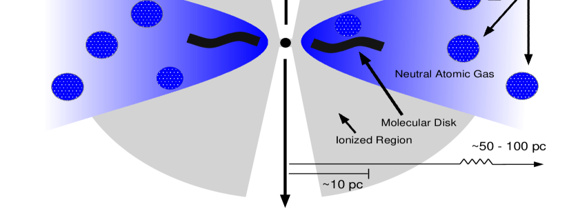
Figure 8: Cartoon model of the environment around an AGN.

In Fig. 8 a simple cartoon schematic for the AGN environment is shown. The details of the equatorial region are based on discussions in Peck, Taylor & Conway (1999). According to unified schemes (see for example the review by Antonucci 1993), core-dominated quasars are viewed such that the jet axis makes only a small angle to the line-of-sight, and they therefore exhibit one-sided jets, apparent superluminal motions, and broad optical emission lines. While jet components are within $\sim$100 pc of the center of activity they are viewed through ionized gas which acts as a Faraday screen. Once the jet components move farther from the nuclear environment the RM rapidly drops.

An observer looking at an AGN nearly edge-on through the denser, multi-phase disk would likely see a galaxy with narrow optical emission lines and symmetric parsec-scale radio structures. The much smaller ($\sim$1 pc) broad line region is hidden from view by the molecular disk. While the cores of lobe-dominated FR II radio galaxies (generally unified with quasars) have not yet been observed with VLBI polarimetry, there is another class of bright sources known as Compact Symmetric Objects that are likely to be youthful versions of FR II radio galaxies (Readhead et al. 1996). For the CSOs, which often have intrinsic sizes less than $\sim$100 pc, all the components will be viewed through a dense multi-phase medium and extremely high RMs ($>>$ 50000 radians m^-2) are therefore to be expected if the model shown in Fig. 8 is correct. Unfortunately such extreme RMs will depolarize the radio source and hence cannot be measured directly. Recent VLBA polarimetry of 20 CSOs by Peck & Taylor (1999) place typical limits on the fractional polarization in CSOs of $<$1%. No polarized flux on the parsec-scale has ever been reported for a CSO.

An observer looking at an AGN even closer to the jet axis than the optimal angle for apparent superluminal motions (1/$\gamma$, where $\gamma$ is the Lorentz factor of the jet) would see slower motions, and greater Doppler beaming. BL Lac objects are even more highly core dominated than quasars. There is some evidence that BL Lac objects have smaller apparent motions than quasars (Gabuzda et al. 1994, Britzen et al. 1999). BL Lac objects have also been observed to have more strongly polarized cores (Gabuzda et al. 1992) compared to quasar cores. This might be achieved if the relativistic jet evacuates a cone through the ionized gas in the nuclear region such that cores of BL Lacs are not viewed through a Faraday screen (see Fig. 8). In fact from lower resolution studies we already know that the BL Lac cores (which dominate over the jet in integrated polarization) must have moderate to low RMs (Rusk 1988; Gabuzda et al. 1992). Future studies of the RM distribution of BL Lac objects on the parsec scale will be of interest to directly confirm these low RMs.

If the RM observed in the core and inner jets is dependent on the orientation of the source as suggested above, then it might be expected to correlate with another orientation dependent parameter, such as $R$ – the ratio of the core flux density to the lobe flux density at an emitted frequency of 5 GHz. Here the term “core flux density” refers to the arcsecond-scale core which includes all the VLBI components. Figure 9 shows the RM plotted against $R$ for the 8 quasars studied in this paper and in paper I. Although 3C 345 has both the lowest RM and the highest measured $R$ value, the results for the sample as a whole are inconclusive. One oddity is the high RM, but lack of any kpc-scale extended emission around 2134+004, even though the core component is not dominant on the parsec-scale like it is for the rest of the sources shown. Indeed computing $R$ on the basis of the parsec-scale emission ($-$0.5) would shift this point to the top-left corner of the plot. I suggest that the lack of extended emission for 2134+004 is due to an intrinsically small size. If 2134+004 is viewed at a larger angle to the line-of-sight then one also expects much slower apparent motion in the jet. Slow motion has been confirmed in 2134+004 ($<$4 c – K. Kellermann, private communication), in sharp contrast to the average speeds of 12 – 14 c reported for 3C 345, 3C 380 and 3C 273 (Vermeulen & Cohen 1994 and references therein).

6 Conclusions

A sample of 40 strong, compact AGN is identified for a multi-frequency polarimetric study. These observations allow imaging of the Faraday Rotation Measure distribution on the parsec scale. This is a relatively new way of probing the AGN environment. Rest frame Faraday Rotation Measures in excess of 1000 radians m^-2 are found in the nuclear regions of 7 out of the 8 quasars studied so far. In all cases the high RMs are confined to the nuclear region within a projected distance of 20 pc of the center of activity. The high RMs seen in these sources probably originate in the same region that produces the narrow optical emission lines. There is some indication that higher nuclear RMs are seen when an AGN is viewed at larger angles to the line of sight, and that correspondingly the lowest nuclear RMs are seen when the line-of-sight is closely aligned to the jet axis. These findings are consistent with the predictions of unified schemes, but the details of the correlation of the nuclear RM with other orientation-dependent observables are as yet unclear. Further multi-frequency polarimetric observations are needed for the remainder of the sample.

Figure 1: (a) Polarized intensity electric vectors (1 mas = 5 mJy/beam; vectors not corrected for Faraday rotation) overlaid on total intensity contours for 1928+738 at 15 GHz. Contours are plotted at $-$2, 2, 4, … 2048 mJy/beam with negative contours shown dashed. The restoring beam is plotted in the lower left corner and has dimensions 1.7 $\times$ 1.1 mas in position angle $-$2.6°. The bullets ($\bullet$) indicate representative points where the rotation measure fit has been plotted. (b) The electric vector position angle as a function of $\lambda^{2}$ between 8 and 15 GHz and the derived RM fits for the points shown in (a).

Figure 2: (a) Polarized intensity electric vectors (1 mas = 3.1 mJy/beam; vectors not corrected for Faraday rotation) overlaid on total intensity contours for 3C 395 at 15 GHz. Contours are plotted at $-$1.5, 1.5, 3, … 768 mJy/beam with negative contours shown dashed. The restoring beam is plotted in the lower left corner and has dimensions 2.1 $\times$ 1.2 mas in position angle $-$4.4°. The bullets ($\bullet$) indicate representative points where the rotation measure fit has been plotted. (b) The electric vector position angle as a function of $\lambda^{2}$ between 8 and 15 GHz and the derived RM fits for the points shown in (a).

Figure 3: (a) Polarized intensity electric vectors (1 mas = 12.5 mJy/beam; vectors not corrected for Faraday rotation) overlaid on total intensity contours for the inner core and jet of 2134+004 at 15 GHz. Contours are plotted at $-$10, 10, 20, … 2560 mJy/beam with negative contours shown dashed. The restoring beam is plotted in the lower left corner and has dimensions 2.8 $\times$ 1.3 mas in position angle $-$2.6°.

Figure 4: (a) Polarized intensity electric vectors (1 mas = 12.5 mJy/beam; vectors not corrected for Faraday rotation) overlaid on total intensity contours for 2230+114 at 15 GHz. Contours are plotted at $-$6, 6, 12, … 3072 mJy/beam with negative contours shown dashed. The restoring beam is plotted in the lower left corner and has dimensions 2.6 $\times$ 1.4 mas in position angle 6°. The bullets ($\bullet$) indicate representative points where the rotation measure fit has been plotted. (b) The electric vector position angle as a function of $\lambda^{2}$ between 5 and 8 GHz and the derived RM fits for the points shown in (a).

Figure 5: (top) Polarized intensity electric vectors (1 mas = 100 mJy/beam; vectors not corrected for Faraday rotation) overlaid on total intensity contours for 3C 279 at 15 GHz at epochs 1997.07 and 1998.59. Contours are plotted at $-$50, 50, 100, … 10240 mJy/beam with negative contours shown dashed. The restoring beam is plotted in the lower left corner and has dimensions 2.5 $\times$ 1.0 mas in position angle 0°. The bullets ($\bullet$) indicate representative points where the rotation measure fit has been plotted. (bottom) The electric vector position angle as a function of $\lambda^{2}$ between 8 and 15 GHz and the derived RM fits.

Figure 7: Projected magnetic field vectors (corrected for the RMs shown in Fig. 6) for 1928+738, 3C 395, 2134+004, and 2230+114 with contours of total intensity superimposed. Contours are as in Figures 1, 2, 3, and 4.

Figure 9: The maximum RM observed in the core (corrected by (1+z)²) for each source plotted against $R$, the ratio of the kpc-scale core flux density to that of the kpc-scale extended emission at an emitted frequency of 5 GHz. Values for $R$ have been taken from Vermeulen & Cohen (1994), except for the upper limit on 2134+004 which was computed using the NVSS image (Condon et al. 1998).

References

- (1)
- (2) Aller, M. F., Aller, H. D., & Hughes, P. A. 1994, in Compact Extragalactic Radio Sources, eds. J.A. Zensus, and K.I. Kellermann, (NRAO), p.185.
- (3) Antonucci, R. 1993, ARA&A, 31, 473
- (4) Blandford, R. D., & Königl, A. 1979, ApJ, 232, 34
- (5) Britzen, S., Vermeulen, R. C., Taylor, G. B., Readhead, A. C. S., Pearson, T. J., Henstock, D. R., & Wilkinson, P. N. 1999, BL Lac Phenomenon, a conference held 22-26 June, 1998 in Turku, Finland, p. 431.
- (6) Cawthorne, T. V., Wardle, J. F. C., Roberts, D. H., Gabuzda, D.C., & Brown, L. F. 1993, ApJ, 416, 496
- (7) Condon, J. J., Cotton, W. D., Greisen, E. W., Yin, Q. F., Perley, R. A., Taylor, G. B., & Broderick, J. J. 1998, AJ, 115, 1693
- (8) Cotton, W. D., Fanti., C., Fanti, R., Dallacasa, D., Foley, A. R., Schilizzi, R. T., & Spencer, R. E. 1997, A&A, 325, 493
- (9) Eckart, A., Witzel, A., Biermann, P., Pearson, T. J., Readhead, A. C. S., & Johnston, K. J. 1985, ApJ, 296, L23
- (10) Gabuzda, D. C., Cawthorne, T. V., Roberts, D. H., & Wardle, J. F. C. 1992, ApJ, 388, 40
- (11) Gabuzda, D. C., Mullan, C. M., Cawthorne, T. V., Wardle, J. F. C., & Roberts, D. H. 1994, ApJ, 435, 140
- (12) Gelderman, R., & Whittle, M. 1994, ApJS, 91, 491
- (13) Gottlieb, E. W., & Liller, W. 1978, ApJ, 222, L1.
- (14) Hummel, C. A. et al. 1992, A&A, 257, 489
- (15) Impey, C. G., & Neugebauer, G. 1988, AJ, 95, 307
- (16) Kellermann, K. I., Clark, B. G., Bare, C. C., Rydbeck, O., Ellder, J., Hansson, B., Kollberg, E., Hoglund, B., Cohen, M. H., & Jauncey, D. L. 1968, ApJ, 153, L209
- (17) Kellermann, K. I., Vermeulen, R. C., Zensus, J. A., & Cohen, M. H. 1998, AJ, 115, 1295
- (18) Kühr, H., Witzel, A., Pauliny-Toth, I. I. K., & Nauber, U. 1981, A&AS, 45, 367
- (19) Lara, L., Muxlow, T. W. B., Alberdi, A., Marcaide, J. M., Junow, W., & Saikia, D. J. 1997, A&A, 319, 405
- (20) Lawrence, C. R., Zucker, J. R., Readhead, A. C. S., Unwin, S. C., Pearson, T. J., & Xu, W. 1996, ApJS, 107, 541
- (21) Lobanov, A. 1996, Ph.D. thesis, New Mexico Institute of Mining and Technology
- (22) Pauliny-Toth, I. I. K., Zensus, J. A., Cohen, M. H., Alberdi, A., & Schaal, R. 1990, in Parsec-Scale Radio Jets, eds. J. A. Zensus & T. J. Pearson, Cambridge, p.55
- (23) Pearson, T. J., & Readhead, A. C. S. 1988, ApJ, 328, 114
- (24) Peck, A. B., & Taylor, G. B. 1999, ApJ, submitted
- (25) Peck, A. B., Taylor, G. B., & Conway, J. E. 1999, ApJ, 521, 103
- (26) Rantakyrö, F. T., Baath, L. B., Dallacasa, D., & Wehrle, A. E. 1996, A&A, 310, 66
- (27) Readhead, A. C. S., Taylor, G. B., Pearson, T. J., & Wilkinson, P. N. 1996, ApJ, 460, 634
- (28) Ros, E., Marcaide, J. M., Guirado, J. C., Ratner, M. I., Shapiro, I. I., Krichbaum, T. P., Witzel, A., & Preston, R. A. 1999, A&A, in press
- (29) Rusk, R. 1988, Ph.D. thesis, University of Toronto
- (30) Scholomitski, G. B. 1965, SovAJ, 9, 3, 516
- (31) Schwab, F. R., & Cotton, W. D. 1983, AJ, 88, 688
- (32) Shepherd, M. C., Pearson, T. J., & Taylor, G. B. 1994, BAAS, 26, 987
- (33) Shepherd, M. C. 1997, in Astronomical Data Analysis Software and Systems VI, A.S.P. Vol. 125, eds. G. Hunt & H. E. Payne, p. 77
- (34) Simard-Normandin, M., Kronberg, P. P., & Button, S. 1981, ApJS, 45, 97
- (35) Stickel, M., Meisenheimer, K., & Kühr, H. 1994, A&AS, 105, 211
- (36) Taylor, G. B., & Perley, R. A. 1993, ApJ, 416, 554
- (37) Taylor, G. B., ApJ, 506, 637 (Paper I)
- (38) Udomprasert, P. S., Taylor, G.B., Pearson, T.J., & Roberts, D.H. 1997, ApJL, 483, L9
- (39) Vermeulen, R. C., & Cohen, M. H., ApJ, 430, 467
- (40) Wrobel, J. M. 1993, AJ, 106, 444