Quasi-periodic X-ray Flares from the Protostar YLW15

Abstract

With ASCA, we have detected three X-ray flares from the Class I protostar YLW15. The flares occurred every $\sim$20 hours and showed an exponential decay with time constant 30–60 ks. The X-ray spectra are explained by a thin thermal plasma emission. The plasma temperature shows a fast-rise and slow-decay for each flare with $kT_{peak}\sim$ 4–6 keV. The emission measure of the plasma shows this time profile only for the first flare, and remains almost constant during the second and third flares at the level of the tail of the first flare. The peak flare luminosities $L_{X,peak}$ were $\sim$ 5–20 $\times 10^{31}$ erg s^-1, which are among the brightest X-ray luminosities observed to date for Class I protostars. The total energy released in each flare was 3–6$\times$10³⁶ ergs. The first flare is well reproduced by the quasi-static cooling model, which is based on solar flares, and it suggests that the plasma cools mainly radiatively, confined by a semi-circular magnetic loop of length $\sim 14\,R_{\odot}$ with diameter-to-length ratio $\sim 0.07$. The two subsequent flares were consistent with the reheating of the same magnetic structure as of the first flare. The large-scale magnetic structure and the periodicity of the flares imply that the reheating events of the same magnetic loop originate in an interaction between the star and the disk due to the differential rotation.

1. Introduction

Low-mass Young Stellar Objects (YSOs) evolve from molecular cloud cores through the protostellar (ages $\sim$10^4-5 yr), the Classical T Tauri (CTTS: $\sim$ 10⁶ yr) and Weak-lined T Tauri (WTTS: $\sim$10⁷ yr) phases to main sequence. Protostars are generally associated with the Class 0 and I spectral energy distributions (SEDs), which peak respectively in the millimeter and infrared (IR) bands. Bipolar flows are accompanied with this phase, suggesting dynamic gas accretion. CTTSs have still circumstellar disks though they have expelled or accreted the infalling envelopes. They are associated with the Class II spectra, which peak at the near-IR. Finally, as the circumstellar disk disappears, YSOs evolve to WTTSs, associated with Class III stars. Early stellar evolution is reviewed by Shu, Adams, & Lizano (1987) and André & Montmerle (1994).

The Einstein Observatory discovered that T Tauri Stars (TTSs), or Class II and Class III infrared objects, are strong X-ray emitters, with the luminosities of 100–10000 times larger than solar flares. These X-rays showed high amplitude time variability like solar flares. The temperature ($\sim$1 keV) and plasma density ($n_{e}\sim$10¹¹cm^-3) are comparable to those of the Sun, hence the X-ray emission mechanism has been thought to be a scaled-up version of solar X-ray emission; i.e., magnetic activity on the stellar surface enhanced by a dynamo process (Feigelson & DeCampli 1981; Montmerle et al. 1983). X-ray and other high energy processes in YSOs are reviewed by Feigelson & Montmerle (1999).

In contrast to TTSs, Class I infrared objects are generally surrounded by circumstellar envelopes of $A_{V}$ up to $\sim$ 40 or more, hence are almost invisible in the optical, near infrared and even soft X-ray bands. The ASCA satellite, sensitive to high energy X-rays up to 10 keV which can penetrate heavy absorption, has found X-rays from Class I objects in the cores of the R CrA, $\rho$ Oph, and Orion clouds at the hard band ($>$ 2 keV) (Koyama et al. 1994; Koyama et al. 1996; Kamata et al. 1997, Ozawa et al. 1999). Even in the soft X-ray band, deep exposures with the ROSAT Observatory detected X-rays from YLW15 in $\rho$ Oph (Grosso et al. 1997) and CrA (Neuhäuser & Preibisch 1997).

A notable aspect of these pioneering observations was the discovery of X-ray flares from Class I stars. ROSAT discovered a giant flare from the protostar YLW15 with total luminosity (over the full X-ray band) of 10^34-36erg s^-1, depending on the absorption. ASCA observed more details of X-ray flares from protostars EL29 in the Opiuchus, R1 in the R CrA core, and SSV63E+W in the Orion, which are associated with larger $N_{H}$ $\simeq$ 10^22-23 cm^-2 than seen in TTSs.

All these findings led us to deduce that greatly enhanced magnetic activity, already well-established in older TTSs, is present in the earlier protostellar phase. Stimulated by these results, and to search for further examples of the protostellar activity in the X-ray band, we have performed an extensive follow-up observation of a core region in $\rho$ Oph, with several Class I X-ray sources. The follow-up observation was made with ASCA 3.5 years after the first observation (Koyama et al. 1994, Kamata et al. 1997). Some previously bright Class Is became dim, while other Class Is were identified as hard X-ray sources. This paper discusses the brightest hard X-ray source, YLW15, concentrating on the characteristics and implications of its peculiar time behavior: quasi-periodic hard X-ray flares. For comparison with previous results, we assume the distance to the $\rho$ Oph region to be 165 pc (Dame et al. 1987) throughout of this paper, although new Hipparcos data suggest a closer distance $d\sim 120$ pc (Knude & Hog 1998).

2. Observation

We observed the central region of $\rho$ Oph cloud with ASCA for $\approx$100 ks on 1997 March 2–3. The telescope pointing coordinates were $\alpha$(2000) = 16h 27.4m and $\delta$(2000) = $-$24^∘ 30^′. All four detectors, the two Solid-state Imaging Spectrometers (SIS 0, SIS 1) and the two Gas Imaging Spectrometers (GIS 2, GIS 3) were operating in parallel, providing four independent data sets. Details of the instruments, telescope and detectors are given by Burke et al. (1991), Tanaka, Inoue, & Holt (1994), Serlemitsos et al. (1995), Ohashi et al. (1996), Makishima et al. (1996), and Gotthelf (1996).

Each of the GIS was operated in the Pulse Height mode with the standard bit assignment that provides time resolutions of 62.5 ms and 0.5 s for high and medium bit rates, respectively. The data were post-processed to correct for the spatial gain non linearity. Data taken at geomagnetic rigidities lower than 6 GV, at elevation angles less than 5^∘ from the Earth, and during passage through the South Atlantic Anomaly were rejected. After applying these filters, the net observing time for both GIS 2 and GIS 3 was 94 ks.

Each of the SIS was operated in the 4-CCD/Faint mode (high bit rate) and in the 2-CCD/Faint mode (medium bit rate). However, we concentrate on the 4-CCD/Faint results in this paper since YLW15 is out of the 2-CCD field of view. The data were corrected for spatial and gain non-linearity, residual dark distribution, dark frame error, and hot and flickering CCD pixels using standard procedures. Data were rejected during South Atlantic Anomalies and low elevation angles as with GIS data. In order to avoid contamination due to light leaks through the optical blocking filters, we excluded data taken when the satellite viewing direction was within 20^∘ of the bright rim of the Earth. After applying these filters, the net observing time for the 4-CCD mode was 61 ks for SIS 0 and 63 ks for SIS 1.

Towards the end of this observation, we detected an enormous flare from T Tauri star ROXs31 which is located close to YLW15 (see §3.1, source 6 in Figure 1). The peak flux of ROXs31 is 1–2 orders of magnitude larger than YLW15 (see §4.2), and its broad point spread function contaminates YLW15 during the flare. Therefore, we excluded the GIS and SIS data taken during the flare of ROXs31 in all analysis of YLW15.

3. Results and Analysis

3.1. Images

Figure 1 shows X-ray images of the $\rho$ Ophiuchi Core F region in the two different energy bands (left panel: 0.7–2 keV, right panel: 2–10 keV), obtained with SIS detectors. Class I sources are indicated by crosses. Since the absolute ASCA positional errors can be as large as 40^′′ for SISs (Gotthelf 1996), we compared the ASCA peak positions to the more accurately known IR positions of two bright sources in the SIS field, ROXs21 (source 5) and ROXs31 (source 6), which are indicated by filled circles in Figure 1 left panel. To obtain the ASCA peak positions, we executed a two-dimensional fitting in the 0.7–2 keV band; we fitted these sources with a position-dependent point spread function in the 0.7–2 keV band and a background model. This procedure was done in the Display45 analysis software package (Ishisaki et al. 1998). The position of ROXs31 was based on the flare phase of this source, while the position of ROXs21 is based on the data before the flare of ROXs31. IR positions are provided by Barsony et al. (1997). The ASCA SIS positions had an average offset (weighted mean by photon counts) of $+$0.18 s in right ascension and $-$7.4^′′ in declination from the IR frame. This positional offset is corrected in Figure 1. After the boresight error correction, remaining excursions between the X-ray and IR positions are 5.5^′′ (rms), which is consistent with the SIS position uncertainty for point sources (Gotthelf 1996). We take the systematic positional error to be 5.5^′′.

From the 2–10 keV band image, we find that the X-ray fluxes from Class I protostars EL29 and WL6 (sources 3 and 4 in Figure 1, right panel) are fainter by one third and less than one third, respectively, comparing to those in the first ASCA observation made in August 1993 (Kamata et al. 1997). The brightest X-ray source in the 2–10 keV band is an unresolved source at $\alpha$(2000) = 16h 27m 27.0s and $\delta$(2000) = $-$24^∘ 40^′ 50^′′ in the position corrected frame. We derived this peak position by the two-dimensional fitting in 2–10 keV band. Since the statistical error is 1^′′, the overall X-ray error (including the systematic error) is $\pm 6^{\prime\prime}$.

The closest IR source is YLW15 with VLA position of $\alpha$(2000) = 16h 27m 26.9s and $\delta$(2000) = $-$24^∘ 40^′ 49.8^′′ ($\pm 0.5^{\prime\prime}$; Leous et al. 1991), located 1.5^′′ away from the X-ray source. The next nearest source is GY263 with IR position of $\alpha$(2000) = 16h 27m 26.6s and $\delta$(2000) = $-$24^∘ 40^′ 44.9^′′ ($\pm$1.3^′′; Barsony et al. 1997). The source is located 5.5^′′ from the X-ray position on the border of the X-ray position error circle. Thus we conclude that the hard X-rays are most likely due to the Class I source YLW15.

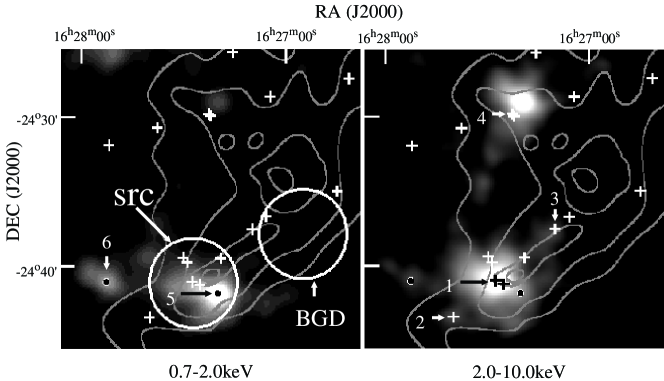
Figure 1.— The SIS images of the central region of $\rho$ Oph cloud in the 0.7–2 keV (left) and the 2–10 keV band (right). The contours are C¹⁸O(1$\rightarrow$0) column densities (Wilking & Lada 1983) in units of 10¹⁶cm^-2, from 1.0 to 2.5 in steps of 0.5, corresponding to $A_{V}\sim$30, 50, 70, 100, respectively. Class I sources are indicated by crosses (Chen et al. 1995, 1997; Motte, André, & Neri 1998). The bright sources 5 and 6 in the 0.7–2 keV band are T Tauri star ROXs21 and ROXs31, respectively. In the 2–10 keV band image, the brightest source is Class I source YLW15 (source 1). Two older Class I sources, IRS51 (source 2) and EL29 (source 3), which have flat SEDs are also detected with a criterion of S/N $\geq$ 5$\sigma$. EL29 and WL6 (source 4) are faint, though both of them emitted strong X-rays in the first ASCA observation (Koyama et al. 1994, Kamata et al. 1997). The hard X-ray source near WL6 is a cluster of T Tauri stars (WL3, WL4, WL5; Wilking & Lada 1983). The source region and background region for YLW15 are also shown by circles.

3.2. X-ray Lightcurve of YLW15

We extracted a lightcurve from a $3^{\prime}$ radius circle around the X-ray peak of YLW15 (see Figure 1). Before the enormous flare from T Tauri star ROXs31, which occurred in the last phase of this observation (see §2), we detected another large flare from Class II source SR24N, located about $7^{\prime}$ away from YLW15 in the GIS field of view. To subtract the time variable contamination from the SR24N in the extended flux of YLW15, we selected a $3^{\prime}$ radius background region (see Figure 1), equidistant from SR24N and YLW15. On the other hand, using such a background, we cannot exclude the contamination from ROXs21 (source 5 in Figure 1), which is 2 arcmin apart from YLW15. Since the X-rays from ROXs21 are dominant below 2 keV (see §3.3 and Fig.3), we examine time variability only in the hard X-ray band ($>$ 2 keV) in which the flux is dominated by YLW15.

Figure 2 (upper panel) shows the background-subtracted lightcurve in the 2–10 keV band with the sum of the SIS (SIS 0 and 1) and GIS (GIS 2 and 3) images. The lightcurve shows a sawtooth pattern with three flares. The peak fluxes of the flares become successively less luminous. Each flare exhibits a fast-rise and an exponential decay with an $e$-folding time of 31$\pm 1$ ks ($\chi^{2}/d.o.f.$ = 61/46), 33$\pm 3$ ks (80/47), and 58${}_{-13}^{+24}$ ks (33/24), for the first, the second, and the third flares, respectively. We show the best fit lightcurves for the second and the third flares with dashed lines, and show the best-fit quasi-static model (see §4.1.1) for the first flare with a solid line in Figure 2 upper panel.

Upper panel: Background-subtracted lightcurve of YLW15 obtained with all the detectors (SIS 0 + SIS 1 + GIS 2 + GIS 3) in the 2–10 keV band. All time bins are 1024 s wide. Middle panel: Time profile of the best-fit temperature. The error bars indicate 90% confidence. Lower panel: Same as the middle panel, but for the best-fit emission measure. The solid lines during Flare I are the best-fit quasi-static model, and the dashed lines during Flare II and III are the best-fit exponential model (see Table 2). One reheating plasma loop is assumed in both cases. Dotted lines during Flare II and III in the upper panel show each flare component without the contribution of the other flares, under assumption that the three flares occurred independently (see §4.1). Asterisks show the average of the model during one time bin. The time axis starts at 00:00:00.0 UT (1997 March 2).

3.3. Time-Sliced Spectra of YLW15

To investigate the origin of the quasi-periodic flares, we made time-sliced spectra for the time intervals given in Figure 2. We extracted the source and background data for each phase from the same regions as those in the lightcurve analysis (see §3.2 and Figure 1). We found that all the spectra show a local flux minimum at $\approx$1.2 keV. For example, we show the spectra obtained with SISs at phases 1 and 8 in Figure 3. This suggests that the spectra have two components, one hot and heavily absorbed, the other cool and less absorbed.

Then we examined possible contamination from the bright, soft X-ray source ROXs21 (source 5 in Figure 1). We extracted the spectrum of ROXs21 from a $2^{\prime}$ radius circle around its X-ray peak. We extracted the data only during phase 1, in order to be free from contamination from the flare on SR24N, which occurred during phases 4–6 (see §3.2). The background data for ROXs21 were extracted from a $2^{\prime}$ radius circle equidistant from YLW15 and ROXs21 during phase 1. After the subtraction of the background, the spectrum of ROXs21 is well reproduced by an optically thin thermal plasma model of about 0.6 keV temperature with absorption fixed at $N_{\rm H}=$1.3$\times$10²¹ cm^-2 ($A_{V}$ = 0.6 mag; Bouvier and Appenzeller 1992) with $\chi^{2}/d.o.f.$ = 17/23. The flux of the soft component of YLW15 is about 30% of the flux of ROXs21, which is equal to the spill-over flux from ROXs21. Thus the soft X-ray component found in YLW15 spectra is due to contamination from the nearby bright source ROXs21.

Having obtained the best-fit spectrum for ROXs21, we fitted the spectrum of YLW15 in each phase with a two-temperature thermal plasma model. The cool component is set to the contamination from ROXs21, and the hot component is from YLW15. For YLW15, free parameters are temperature ($kT$), emission measure ($EM$), absorption ($N_{\rm H}$) and metal abundance. For ROXs21, $EM$ is the only free parameter and the other parameters are fixed to the best-fit values obtained in phase 1. We found no significant variation in $N_{\rm H}$ of YLW 15 from phase to phase, hence, we fixed the $N_{\rm H}$ to the best-fit value at phase 1. The resulting best-fit parameters of YLW15 for each time interval are shown in Table 1. The best-fit spectra of phases 1 and 8 are illustrated in Figure 3, and the time evolution of the best-fit parameters are shown in Figure 2.

The SIS (SIS 0 + 1) spectra of YLW15 at phase 1 and 8 (see Figure 2). The solid lines show the best-fit two-temperature coronal plasma model derived from simultaneous fitting of GIS and SIS data. Lower panel shows the residuals from the best-fit model.

Table 1Best-fit parameters to the spectra of YLW15^a.

Phaseb	$kT$	Abundance	$EM^{c}$	$L_{\rm X}^{d}$	$\chi^{2}$/d.o.f
	(keV)	(solar)	(1054cm-3)	(1031erg s-1)
1	5.6${}^{+1.3}_{-1.0}$	0.4${}^{+0.2}_{-0.1}$	7.2${}_{-0.8}^{+1.1}$	15$\pm$1	181/106
2	4.4${}^{+0.8}_{-0.7}$	0.4${}^{+0.2}_{-0.2}$	3.4${}_{-0.3}^{+0.4}$	6.0$\pm$0.7	191/164
3	2.9${}^{+0.5}_{-0.3}$	0.7${}^{+0.5}_{-0.4}$	2.1${}_{-0.3}^{+0.4}$	3.4$\pm$0.8	80/84
4	5.3${}^{+1.6}_{-1.1}$	0.6${}^{+0.4}_{-0.4}$	2.7${}_{-0.3}^{+0.4}$	5.6$\pm$0.8	55/52
5	2.3${}^{+0.4}_{-0.3}$	0.5${}^{+0.6}_{-0.4}$	3.2${}_{-0.7}^{+0.8}$	4.4$\pm$1.3	163/138
6	1.6${}^{+0.3}_{-0.3}$	$<$1.3	2.3${}_{-1.2}^{+1.5}$	2.5$\pm$1.5	46/40
7	4.2${}^{+1.5}_{-0.9}$	$<$0.4	2.2${}_{-0.3}^{+0.4}$	3.5$\pm$0.5	153/139
8	3.0${}^{+0.9}_{-0.5}$	0.7${}^{+1.3}_{-0.5}$	1.7${}_{-0.4}^{+0.4}$	2.9$\pm$0.6	59/65

Note. — The errors are at 90% confidence level.

^a Absorption column density is fixed to the best fit value for phase 1, 3.3$\times 10^{22}$ cm^-2.

^b see Figure 2.

^c Emission Measure, $\int n_{e}^{2}dV$ ($n_{e}$: electron density, $V$: emitting volume).

^d Absorption-corrected X-ray luminosity in the 0.1 – 100 keV band.

4. Discussion

In this observation, we detected hard X-rays ($>$ 2 keV) from the Class I source YLW15 for the first time; the source was not detected in the first ASCA observation executed 3.5 years later (Kamata et al. 1997). On the other hand, the Class I sources EL29 and WL6, which emitted bright hard X-rays in the first observation, became very faint (see §3.1). Then we conclude that hard X-rays from Class I protostars in the $\rho$ Oph cloud are highly variable in the time spans, and we suspect that the non-detection of hard X-rays from other Class I objects is partly due to the long-term time variability. From YLW15, we discovered a peculiar time behavior: quasi-periodic flares. We shall now discuss the relation between each flare from YLW15 and the physical conditions.

4.1. Physical Parameters of the Triple Flare

If the three intermittent flares are attributed to a single persistent flare, with the three events due to geometrical modulation, such as occultation of the flaring region by stellar rotation or orbit in an inner disk, then only the emission measure should have shown three peaks. The temperature would have smoothly decreased during the three flares. However, in our case, we see the temperature following the same pattern as the luminosity, decreasing after each jump, as indicated in Table 1 and Figure 2 middle panel. To test further, we fitted the temperatures in phases 1–8 with a single exponential decay model, and confirmed that it is rejected with 89 % confidence. We then interpret the variability of YLW15 as due to a triple flare, in which each flare followed by a cooling phase. Now, let us label phases 1–3, 4–6, and 7–8 as Flare I, II, and III, respectively. In this subsection we will use the cooling phases to estimate the physical conditions of the plasma in each flare. Details are given in the Appendix.

4.1.1 Flare I

Here we assume that the plasma responsible for Flare I is confined in one semi-circular magnetic loop with constant cross section along the tube flux, with length $L$, and diameter-to-length (aspect) ratio $a$, based on the general analogy of solar-type flares. To the decay of Flare I, we apply a quasi-static cooling model (van den Oord & Mewe 1989), in which the hot plasma cools quasi-statically as a result of radiative (90 %) and conductive (10 %) losses (see detailed comment in Appendix §1). If the cooling is truly quasi-static, $T^{13/4}/EM$ shows constant during the decay (where $T$ is plasma temperature and $EM$ is the emission measure). We find for the three successive bins (phases 1–3) of Flare I that $(T/10^{7}\,{\rm K})^{13/4}/(EM/10^{54}\,{\rm cm}^{-3})=61\pm 55,~{}59\pm 42,~{}25\pm 18$, which are not inconsistent with a constant value, taking into account the large error bars. Then, fitting our data with the quasi-static model, we find satisfactory values of $\chi^{2}_{red}$ for the count rates, temperature, and emission measure (see panel 1 in Table 2). We conclude that our hypothesis of quasi-static cooling is well verified; an underlying quiescent coronal emission is not required to obtain a good fit. The best fits are shown by solid lines in Figure 2. From the peak values of $T$ and $EM$, and the quasi-static radiative time scale, we derived loop parameters as listed in Table 3. The detailed procedure is written in Appendix. The aspect ratio $a$ of 0.07 is within the range for solar active-region loops ($0.06\leq a_{\odot}\leq 0.2$, Golub et al. 1980), which supports the assumed solar analogy.

4.1.2 Flares II and III

The appearance of Flare II can be interpreted either by the reheating of the plasma cooled during Flare I, or by the heating of a distinct plasma volume, independent from that of Flare I. In the latter case, the lightcurve and $EM$ would be the sum of Flare I component and new flare component. The $EM$ of the new flare component can be derived by subtracting the component extrapolated from Flare I. The derived $EM$ are 1.6$\pm$0.4 (phase 4), 2.5$\pm$0.8 (phase 5), and 1.9$\pm$1.5 (phase 6). Then we fitted the lightcurve and $EM$ with the quasi-static model assuming the above two possibilities. However, in both of the cases, the model did not reproduce the lightcurve and $EM$ simultaneously, and the quasi-static cooling model cannot be adopted throughout the triple flare but Flare I.

For simplicity, we fitted the parameters in Flare II with an exponential model. The best-fit parameters are shown in Table 2, and each models for the reheating and the distinct flare assumptions are shown by the dashed and the dotted lines in Figure 2, respectively. The obtained $\chi^{2}_{red}$ and the timescale for each lightcurve and $EM$ were similar between the two assumptions. Therefore both of the possibilities cannot be discriminated. As for $EM$, both of the fits show no decay or very long time decay, which is not seen in the usual solar flares. The constant feature in $EM$ makes the quasi-static model unacceptable. Since we cannot derive the aspect ratio of Flare II by fitting with quasi-static cooling model, assuming the ratio derived in Flare I and that radiative cooling is dominant, we deduced the plasma parameters as shown in Table 3. Here, we derived the values assuming the reheating scenario (the former assumption). The results show that the plasma density and the volume remain roughly constant from Flare I. This supports that Flare II resulted from reheating of the plasma created by Flare I.

As for Flare III, because of the poor statistics and short observed period, the fits to lightcurve with the exponential model give no constrain between the above two possibilities. The results are shown in Table 2 and Figure 2. We derived the plasma parameters of Flare III in the same way for Flare II, as shown in Table 3. These values are similar to those in Flare I and II. All these are consistent with the scenario that a quasi-periodic reheating makes the triple flare. The heating interval is $\sim$20 hour. The loop size is approximately constant through the three flares and is as large as $\sim$14 $R_{\odot}$. The periodicity and the large-scale magnetic structure support a scenario that an interaction between the star and the disk occurred by the differential rotation and reheated the same loop periodically (e.g., Hayashi, Shibata, & Matsumoto 1996). The detail will be presented in Paper II (Montmerle et al. 1999).

Table 2Fitting of cooling phase of flares

model expression	${\cal F}$	$\alpha$	${\cal F}_{\mathrm{p}}$	$\tau$	$\chi^{2}_{red}$
				[ks]	(d.o.f.)
[1]	[2]	[3]	[4]	[5]	[6]
${\cal F}_{\mathrm{I,qs}}(t)={\cal F}_{\mathrm{p}}\times\{1+(t-t_{\mathrm{I}})/3\tau\}^{-\alpha}$	$I$ [cnts ks-1]	4	$172\pm 5$	$31\pm 1$	0.8 (45)
	$kT$ [keV]	8/7	$5.6\pm 0.6$	[31]	0.5 (2)
	$EM$ [1054 cm-3]	26/7	$10.4\pm 0.9$	[31]	0.4 (2)
${\cal F}_{\mathrm{II}}(t)={\cal F}_{\mathrm{p}}\times exp\{-(t-t_{\mathrm{II}})/\tau\}$	$I$ [cnts ks-1]	–	$62\pm 3$	$33\pm 3$	1.7 (47)
	$kT$ [keV]	–	$4\pm 1$	$50\pm 20$	1.5 (1)
	$EM$ [1054 cm-3]	–	$3\pm 1$	$>$ 53	0.4 (1)
${\cal F}_{\mathrm{I+II}}(t)={\cal F}_{\mathrm{I,qs}}(t)+{\cal F}_{\mathrm{II}}(t)$	$I$ [cnts ks-1]	–	$46\pm 3$	$29\pm 2$	1.6 (47)
	$EM$ [1054 cm-3]	–	$1.6\pm 0.8$	$>$ 54	0.6 (1)
${\cal F}_{\mathrm{III}}(t)={\cal F}_{\mathrm{p}}\times exp\{-(t-t_{\mathrm{III}})/\tau\}$	$I$ [cnts ks-1]	–	$35\pm 2$	$60\pm 20$	1.4 (24)
	$kT$ [keV]	–	$5\pm 3$	55 ($>$ 16)	$\chi^{2}=0$ (0)
	$EM$ [1054 cm-3]	–	$2.5\pm 0.7$	71 ($>$ 23)	$\chi^{2}=0$ (0)
${\cal F}_{\mathrm{I+II+III}}(t)={\cal F}_{\mathrm{I+II}}(t)+{\cal F}_{\mathrm{III}}(t)$	$I$ [cnts ks-1]	–	$28\pm 2$	$60\pm 20$	1.4 (24)

Note. — Panel 1 gives the quasi-static fit for Flare I. Panel 2 (Panel 3) gives the exponential fit for Flare II (Flare III): first assuming that the flares are reheating of the same plasma volume as the previous flare; second assuming that the three flares are independent (the previous flares contribute to the latter flares). $t_{\mathrm{I}}$, $t_{\mathrm{II}}$, and $t_{\mathrm{III}}$ are the beginning time of Flare I, II, and III, respectively. We assume only positive values for the decay time (Column [5]). The errors are at 90 % confidence level.

Table 3Physical parameters for the triple flare

Flare	$a$	$L$	$n_{e}$	$B$	$L_{X,peak}$	$\tau$	$E_{tot}$
		[R⊙]	[1011 cm-3]	[G]	[1031 erg s-1]	[ks]	[1036 erg]
I	0.07$\pm$0.02	14$\pm$2	0.5$\pm$0.1	150$\pm$20	20$\pm$1	31$\pm$1	6.0$\pm$0.5
II	[0.07$\pm$0.02]	11$\pm$5	0.4$\pm$0.1	120$\pm$30	8$\pm$1	33$\pm$3	2.8$\pm$0.6
III	[0.07$\pm$0.02]	15$\pm$10	0.3$\pm$0.2	100$\pm$60	4.6$\pm$0.5	60$\pm 20$	2.7$\pm$1.0

Note. — $a$: diameter-to-length ratio of the loop; $L$: loop length; $n_{e}$: electron density; $B$: minimum value of the magnetic field confining the loop plasma; $L_{X,peak}$: X-ray luminosity at the flare peak in the 0.1–100 keV band; $\tau$: characteristic decay time of the lightcurve; $E_{tot}$: total energy released during the cooling phase in X-ray wavelength.

4.2. Comparison with Other Flares

Among YSOs, TTSs have been known for strong X-ray time variabilities since the $Einstein$ Observatory discovered them (see §1). At any given moment, 5–10 % are caught in a high-amplitude flare with timescales of hours (Feigelson & Montmerle 1999). The most recent example is that of V773 Tau, which exhibits day-long flares with $L_{X,peak}\sim$ 2–10 $\times 10^{32}$ erg s^-1 and very high temperatures of $\sim 10^{8}$ K (Tsuboi et al. 1998). Other examples of bright TTS X-ray flares are P1724, a WTTS in Orion ($L_{X,peak}\sim 2\times 10^{33}$ erg s^-1; Preibisch, Neuhaüser, & Alcalá 1995), and LkH$\alpha$92, a CTTS in Taurus (Preibisch, Zinnecker, & Schmitt 1993). These X-ray properties resemble those of RS CVn systems.

Recently, a dozen protostars have been detected in X-rays, and four of those showed evidence for flaring (RCrA core; Koyama et al. 1996, EL29; Kamata et al. 1997, YLW15; Grosso et al. 1997, and SSV63 E+W; Ozawa et al. 1999). In the “superflare” of YLW15 (Grosso et al. 1997), an enormous X-ray luminosity was recorded during a few hours. If we adopt the absorption we derived ($N_{H}=$ 3$\times 10^{22}$ cm^-2), the absorption-corrected X-ray luminosity in 0.1–100 keV band is $L_{X,peak}\sim 10^{34}$ erg s^-1. The “triple flare” we detected in this observation does not reach the same level as the “superflare”: $L_{X,peak}=5-20\times 10^{31}$ erg s^-1 in the same X-ray band.

To compare the flare properties of our triple flare from YLW15 with other flare sources, including RS CVns, we selected bright flare sources as seen in Table 4. All the flare sources have a well-determined temperature using a wide range of energy band of $Tenma,Ginga$, and $ASCA$ satellites. Since the samples of YSO flares were less, we added two TTS flares; the flares on ROXs21 and SR24N detected in our observations (see §2 and §3). We analyzed them using GIS data. The densities and volumes for all the sources were derived assuming that radiative cooling is dominant.

As a result, we found that although less energetic than the “superflare”, with total energies in excess of 3–6 $\times 10^{36}$ ergs, the triple flare are on the high end of the energy distribution for protostellar flares. While the plasma densities, temperatures, and then derived equipartition magnetic fields are typical of stellar X-ray flares, the emitting volume is huge; it exceeds those in binary systems of RS CVns by a few orders of magnitude.

Table 4Comparison with the other flares

Source	SED	$n_{e}$	$V$	$\tau$	$kT_{peak}$	$EM_{peak}$	$E_{tot}$	ref.
		[1011 cm-3]	[10${}^{33}\,cm^{3}$]	[ks]	[keV]	[1055 cm-3]	[1036 erg]
YLW15(I)	I	0.5	3	31	6	0.7	6
YLW15(II)	I	0.4	2	33	5	0.3	3
YLW15(III)	I	0.3	2	60	4	0.2	3
EL29	I	1	0.2	8	4	0.3	0.4	(1)
RCrA	I	1	0.04	20	6	0.04	0.2	(2)
SSV63E+W	I	1	2	10	6	2	4	(3)
SR24N	II	5	0.1	6	7	3	6
ROXs31	III	3	0.6	7	6	6	13
ROX7	III	3	0.01	6	3	0.1	0.1	(1)
V773Tau	III	3	0.6	8	10	5	8	(4)
Algol		1	0.09	20	5	0.1	0.6	(5)
$\pi$ Peg		8	0.006	2	6	0.3	0.2	(6)
AU Mic		6	0.002	2	5	0.06	0.03	(7)

Note. — reference: (1) Kamata et al. 1997

(2) Koyama et al. 1996 and Hamaguchi private comm.

(3) Ozawa et al. 1999

(4) Tsuboi et al. 1998

(5) Stern et al. 1992

(6) Doyle et al. 1991

(7) Cully et al. 1993

5. Summary and Conclusions

In the course of a long exposure of the $\rho$ Oph cloud with ASCA, we found evidence for a ‘triple flare’ from the Class I protostar YLW15. This triple flare is the first example of its kind; it shows an approximate periodicity of $\sim 20$ hours. Each event shows a clear decrease in the temperature, followed by reheating, with $kT_{peak}\sim$ 4–6 keV, and luminosity $L_{X,peak}\sim$ 5–20 $\times 10^{31}$ erg s^-1. Apart from the periodicity, the characteristics of the flares are among the brightest X-ray detections of Class I protostars.

A fitting with the quasi-static model (VM), which is based on solar flares, reproduces the first flare well, and it suggests that the plasma cools mainly radiatively, having semi-circular shape with length $\sim 14\,R_{\odot}$ (radius of the circle $R\sim 4.5\,R_{\odot}$) and aspect ratio $\sim 0.07$. The minimum value of the confining field is $B\sim 150$ G. The two subsequent flares have weaker intensity than the first one but consistent with the reheating of basically the same magnetic structure as the first flare. The plasma volume is huge; a few orders of magnitude larger than the typical flares in RS CVns.

The fact that the X-ray flaring is periodic suggests that the cause for the heating is periodic, hence is linked with rotation in the inner parts of the protostar. The large size of the magnetic structure and the periodicity support the scenario that the flaring episode has originated in a star-disk interaction; differential rotation between the star and disk would amplify and release the magnetic energy in one rotation period or less, reheating the flare loop as observed in the second and third flares.

APPENDIX
Determination of the Physical Parameters of the Flares

1. Loop Parameters

We make use of the general treatment for solar-type flares, put forward by van den Oord & Mewe (1989, hereafter VM). The decrease in the thermal energy of the cooling plasma is assumed to be caused by radiative ($\tau_{\mathrm{r}}$) and conductive losses ($\tau_{\mathrm{c}}$): its decay time is thus $1/\tau_{\mathrm{eff}}=1/\tau_{\mathrm{r}}+1/\tau_{\mathrm{c}}$. VM assumed that the flare lightcurve and temperature decrease exponentially with decay times $\tau_{\mathrm{d}}$ and $\tau_{\mathrm{T}}$, respectively. This effective cooling time is related to observed time scales by $1/\tau_{\mathrm{eff}}=7/8\tau_{\mathrm{T}}+1/2\tau_{\mathrm{d}}$. We assume here that the flare occurs in only one semi-circular loop with constant section along the tube flux, radius $R$ ($R=L/\pi$; length $L$), diameter-to-length ratio $a$, and volume $V$. VM gives an expression of $L$ versus $a$, depending on $\tau_{\mathrm{eff}}$, the temperature, the emission measure (hereafter $EM$), and the ratio $\tau_{\mathrm{r}}/\tau_{\mathrm{c}}$. Because of the assumed exponential behavior of the lightcurve and temperature, the moment at which this expression is applied is not important. The only restriction is that both the temperature and the $EM$ started to decrease.

Due to the low statistics, we have only time-sliced values of the temperature and the $EM$. Let us call $t_{i}$ ($t_{f}$) the beginning (end) of the time interval within which the temperature was estimated, we have: $\overline{T}=\int_{t_{i}}^{t_{f}}T(t^{\prime})\,dt^{\prime}/(t_{f}-t_{i})$. We use this relation to find the behavior of the temperature as a function of time.

We now have a relation between $L$ and $a$, but the ratio $\tau_{\mathrm{r}}/\tau_{\mathrm{c}}$ is unknown, and even worse may change during the decay of the flare. An exception to this is when the flare volume cools quasi-statically, evolving through a sequence of quasi-static equilibria, where the loop satisfies scaling laws, and where $\tau_{\mathrm{r}}/\tau_{\mathrm{c}}=cst$. Due to the dependency of $\tau_{\mathrm{r}}$ and $\tau_{\mathrm{c}}$ on the temperature and the $EM$, $\tau_{\mathrm{r}}/\tau_{\mathrm{c}}=cst$ implies $T^{13/4}/EM=cst$. VM gives in that case analytical expressions for several physical quantities versus time, all depending on the quasi-static radiative time scale ($\tau_{\mathrm{r,qs}}$). $\tau_{\mathrm{r,qs}}$ can be estimated from the lightcurve which must be proportional to the radiative loss. The temperature and the $EM$ can be fitted as described above using this value of $\tau_{\mathrm{r,qs}}$, and give the peak values $kT_{\mathrm{p,qs}}$, $EM_{\mathrm{p,qs}}$ (see Col. [4]–[5] in our Table 2, panel 1 for details).

Using an expression for the radiative time (eq.[23a] of VM), the $EM$ (eq.[3] of VM) and the scaling law (SL[2], eq.[196] of VM), we obtained the loop characteristics for the quasi-static model:

$$a=1.38\times(\tau_{\mathrm{r,qs}}/10\,ks)^{-1/2}\times(kT_{\mathrm{p,qs}}/keV)^{-33/16}\times(EM_{\mathrm{p,qs}}/10^{54}\,cm^{-3})^{1/2},$$ (1)

$$L=1.0\,R_{\odot}\times(\tau_{\mathrm{r,qs}}/10\,ks)\times(kT_{\mathrm{p,qs}}/keV)^{7/8},$$ (2)

$$n_{e}=4.4\times 10^{10}\,cm^{-3}\times(\tau_{\mathrm{r,qs}}/10\,ks)^{-1}\times(kT_{\mathrm{p,qs}}/keV)^{3/4}.$$ (3)

Using an expression for the ratio $\tau_{\mathrm{r}}/\tau_{\mathrm{c}}$ on page 252 of VM, we found $\tau_{\mathrm{r}}/\tau_{\mathrm{c}}=\mu\times f$, with the parameter $\mu$ depending only on the exponent of the temperature in the expression for the radiative loss (for temperature above 20 MK, $\mu=0.18$), and the multiplicative function $f$ coming from the expression for the mean conductive energy loss (formula [7] of VM), which is equal to 4/7 for a loop with a constant section. Thus, $\tau_{\mathrm{r}}/\tau_{\mathrm{c}}=0.1$. In other words, the quasi-static model implies that 91 $\%$ of the lost energy are radiative losses: radiation is the dominant energy loss process.

Assuming that the cooling is only radiative we used these simplified relations based on the exponential decay of the lightcurve, the temperature, and the $EM$:

$$n_{e}=4.4\times 10^{10}\,cm^{-3}\times(\tau_{\mathrm{d}}/10\,ks)^{-1}\times(kT_{\mathrm{p}}/keV)^{3/4},\mathrm{~{}for~{}kT>2\,keV},$$ (4)

$$L=7.4\,R_{\odot}\times(a/0.07)^{-2/3}\times(\tau_{\mathrm{d}}/10\,ks)^{2/3}\times(kT_{\mathrm{p}}/keV)^{-1/2}\times(EM_{\mathrm{p}}/10^{54})^{1/3},$$ (5)

with $kT_{\mathrm{p}}$ ($EM_{\mathrm{p}}$) the peak value of the temperature ($EM$).

2. Magnetic Field

Assuming equipartition between the magnetic pressure $B^{2}/8\pi$ and the ionized gas pressure $2n_{e}kT$, we can obtain a minimum value of the magnetic field confining the emitting plasma using:

$$B=28.4\,G\times(n_{e}/10^{10}\,cm^{-3})^{1/2}\times(kT/keV)^{1/2}$$ (6)

3. Released Energy

For estimating the energy released by the flare during its cooling phase we need the peak luminosity value of this flare. As the lightcurve must be proportional to the intrinsic luminosity, we fit the time averaged intrinsic luminosities in the 0.1–100 keV band (given in Table 1) with the same model used for the lightcurve fitting. This gives the peak luminosity, $L_{\mathrm{X,\,peak}}$, and a characteristic decay time $\tau$. Thus, the total energy released by this flare is:

$$E_{\mathrm{tot}}\sim 10^{35}\,erg\times(L_{\mathrm{X,\,peak}}/10^{32}\,erg\,s^{-1})\times(\tau/ks)$$ (7)

References

- Andre & Montmerle (1994) André, P., & Montmerle, T. 1994, ApJ, 420, 837
- Barsony et al. (1997) Barsony, M., Kenyon, S. J., Lada, E. A., & Teuben, P. J. 1997, ApJS, 112, 109
- Bouvier and Appenzeller (1992) Bouvier, J., & Appenzeller, I. 1992, A&AS, 92, 481
- Burke et al. (1991) Burke, B. E., Mountain, R. W., Harrison, D. C., Bautz, M. W., Doty, J. P., Ricker, G. R., & Daniels, P. J. 1991, IEEE Trans. ED-38, 1069
- Chen et al (1995) Chen, H., Myers, P. C., Ladd, E. F., & Wood, D. O. S. 1995, ApJ, 445, 377
- Chen et al (1997) Chen, H., Grenfell, T. G., Myers, P. C., & Hughes, J. D. 1997, ApJ, 478, 295
- Cully et al (1993) Cully, S. L., Siegmund, O. H. W., Vedder, P. W., & Vallerga, J. V. 1993, ApJ, 414, L49
- Dame et al (1987) Dame, T. M. et al. 1987, ApJ, 322, 706
- Doyle et al (1991) Doyle, J. G. et al. 1991, MNRAS, 248, 503
- Feigelson & DeCampli (1981) Feigelson, E. D., & DeCampli, W. M. 1981, ApJ, 243, L89
- Feigelson (1999) Feigelson, E. D., & Montmerle, T. 1999, ARA&A, in press
- Golub et al. (1980) Golub, L., Maxson, C., Rosner, R., Vaiana, G. S. & Serio, S. 1980, ApJ, 238, 343
- Gotthelf (1996) Gotthelf, E. 1996, ASCANEWS (Greenbelt: NASA GSFC), 4, 31
- Grosso et al (1997) Grosso, N., Montmerle, T., Feigelson, E. D., André, P., Casanova, S., & Gregorio-Hetem, J. 1997, Nature, 387, 56
- Hayashi et al (1996) Hayashi, M. R., Shibata, K., & Matsumoto, R. 1996, ApJ, 468, L37
- Ishisaki et al (1998) Ishisaki, Y., Matsuzaki, K., Shirahashi, A., Takahashi, T., & Itoh, R. 1998, Interactive Tool for Data Analysis for DISPLAY45 (version 1.80)
- Kamata et al (1997) Kamata, Y., Koyama, K., Tsuboi, Y., & Yamauchi, S. 1997, PASJ, 49, 461
- Knude et al (1998) Knude, J. & Hog, E. 1998, aap, 338, 897
- Koyama et al (1994) Koyama, K., Maeda, Y., Ozaki, M., Ueno, S., Kamata, Y., Tawara, Y., Skinner, S., & Yamauchi, S., 1994, PASJ, 46, L125
- Koyama et al (1996) Koyama, K., Hamaguchi, K., Ueno, S., Kobayashi, N., & Feigelson, E. D., 1996, PASJ, 48, L87
- Leous et al (1991) Leous, J. A., Feigelson, E. D., André, P., & Montmerle, T., 1991, apj, 379, 683
- Makishima et al. (1996) Makishima, K., et al. 1996, PASJ, 48, 171
- Montmerle et al (1983) Montmerle, T., Koch-Miramond, L., Falgarone, E., & Grindlay, J. E. 1983, ApJ, 269, 182
- Montmerle et al (1999) Montmerle, T., Grosso, N., Tsuboi, Y., & Koyama, K. 1999, ApJ, submitted
- Motte et al (1998) Motte, F., André, P., & Neri, R. 1998 A&A, 336, 150
- Motte et al (1998) Neuhäuser, R., Preibisch, T. 1997 A&A, 322, L37
- Ohashi et al. (1996) Ohashi, T., Ebisawa, K., Fukazawa, Y., Hiyoshi, K., et al. 1996, PASJ, 48, 157
- Ozawa et al (1999) Ozawa, H., Nagase, F., Ueda, Y., Dotani, T., & Ishida, M. 1999, ApJ, 523, L81
- Preibisch et al (1993) Preibisch, T., Zinnecker, H., & Schmitt, J. H. M. M. 1993, A&A, 279, L33
- Preibisch et al (1995) Preibisch, T., Neuhäuser, R., & Alcala, J. M. 1995, A&A, 304, L13
- van den Oord (1989) van den Oord, G. H. J. & Mewe, R. 1989, A&A, 213, 245
- Serlemitsos et al. (1995) Serlemitsos, P. J., et al. 1995, PASJ, 47, 105
- Shu & Adams (1987) Shu, F. H., Adams, F. C. & Lizano, S. 1987, ARA&A, 25, 23
- Stelzer et al. (1999) Stelzer, B., Neuhäser, R., Casanova, S., & Montmerle, T. 1999, A&A, 344, 154
- Stern et al. (1992) Stern, R. A., Uchida, Y., Tsuneta, S., & Nagase, F. 1992, ApJ, 400, 321
- Tanaka et al. (1994) Tanaka, Y., Inoue, H., & Holt, S. S. 1994, PASJ, 46, L37
- Tsuboi et al. (1998) Tsuboi, Y., Koyama, K., Murakami, H., Hayashi, M., Skinner, & S., Ueno, S. ApJ, 503, 894
- Wilking & Lada (1983) Wilking, B. A., & Lada, C. J. 1983, ApJ, 274, 698