Growing of the Inhomogeneities with Particle Production

Abstract

Perturbations in Prigogine’s cosmological model with particle creation are investigated in the framework of Newtonian gravity theory.

The necessary conditions for the density contrast to reach the non-linear regime which is necessary to guarantee structure formation are obtained.

The upper limit of the age of the universe is investigated for the perturbations obtained to find them compatible with the observed data from COBE(Cosmic Background Explorer satellite).

We compare the particle horizon and the Hubble sphere for to guarantee that the perturbation is in observable universe.

1 Introduction

This paper reviews some aspect of our knowledge of the gravitational theory of fluctuations of density in homogeneous and isotropic models of the universe. The evolution of density perturbation is evaluated for Prigogine’s particle creation model for irreversible process with the framework of Newtonian gravity theory. In this framework various works [1] - [11] study the time dependence for the density contrast. We will find some simple conditions on the rate of expansion which permit hydrodynamic perturbation to grow rapidally with time.

Here, we just assume for compatibility with the cosmological principle, that any fluctuation present must have an amplitude which decreases with length scales or equivalently, mass scale.

The importance of the reach of the non linear regime for the density contrast is relacioned with the age of the structures in the universe. Considering that the structures in the universe to form “from top down”, we can use the period when $\delta_{+}\approx 1$ and the age of the universe to estimate the age for the structures [12].

2 Prigogine’s Model

The universe has a considerable entropy content, mainly in the form of blackbody radiation. Therefore, Einstein equations are purely adiabatic and reversible implying in the raising of the question: What is the origin of cosmological entropy?

Prigogine [13] proposed a new type of cosmological history which includes large scale entropy production. These cosmologies are based on the reinterpretation of the matter-energy tensor in Einstein’s equations and applied to the homogeneous and isotropic universe, namely

$$ds^{2}=dt^{2}-R(t)^{2}d\sigma^{2}\,\,,$$ (1)

R=R(t) only. The Einstein’s field equations

$$G_{\mu\nu}=kT_{\mu\nu}$$ (2)

are used together with the adiabatic transformation in any system for the perfect fluid, namely

$${T}^{\mu\,\nu}=\left(\rho+P\right){u}^{\mu}{u}^{\nu}+P{g}^{\mu\,\nu}\,,$$

where

$$P=P_{c}+P_{th}\,.$$

$P_{th}$ is the thermodynamic pressure and $P_{c}$ corresponds to the matter creation that is defined by [13], namely:

$$P_{c}=-\frac{\rho+P_{th}}{n}(\dot{n}+3Hn)\,.$$ (3)

The process of particle creation is to be consider adiabatic and pressure creation is a kind of viscosity pressure that is present in the energy momentum tensor representing the gravitational fluid. According to the second law of thermodynamic the particle number variations admitted are such that

$$dN=d(nV)\geq 0\,\,.$$ (4)

This implies that, in the presence of matter creation, the usual Einstein’s equation for (1) is:

$$k\rho=3H^{2}+\frac{\kappa}{R^{2}}$$ (5)

$$\dot{\rho}=-3H(\rho+P_{th}),$$ (6)

to become

$$k\rho=3H^{2}+\frac{\kappa}{R^{2}}\,\,,$$ (7)

and

$$\dot{\rho}=\frac{\dot{n}}{n}(\rho+P_{th}).$$ (8)

In order to exemplify the theory mentioned above, they consider the thermodynamical pressure as zero and the source of the matter creation proportional to $H^{2}$. Thus

$$\dot{n}+n\theta=\Psi$$ (9)

to become

$$\frac{1}{R^{3}}\frac{d}{dt}(nR^{3})=\alpha H^{2}\,,$$ (10)

with $\alpha\geq 0$. This leads to

$$R(t)=\{1+c(e^{\frac{\alpha kMt}{6}}-1)\}^{\frac{2}{3}}\,,$$ (11)

where

$$c=\frac{9}{kM\alpha}(\frac{kMn_{0}}{3})^{\frac{1}{2}}\,$$ (12)

$M$ is the mass of particle produced and $n_{0}$ is the initial number density of particles.

The evolution of the scale factor is similar to the models with cosmological term [14] and have the pattern demonstrate in fig.1.

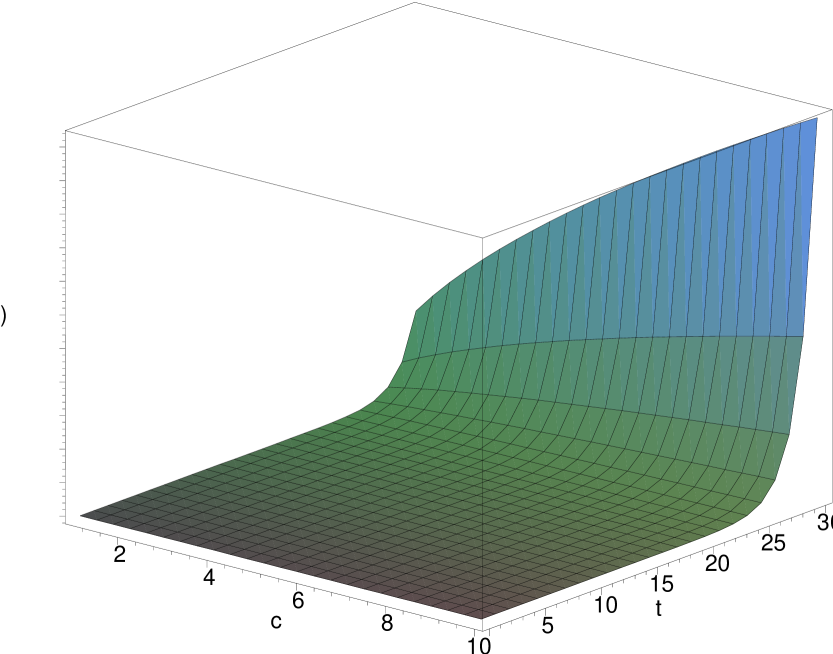
Figure 1: Evolution for the scale factor $\bf{R(t)}\times\bf{t}\times c$   .

Note that the recent measurement of distant supernova when they are used as standard candles [15] [16] indicates an accelerating universe, consequently the desaceleration parameter will establish restrictions on the creation parameters of Prigogine’s model. Namely

$$q=-\frac{\ddot{R}R}{\dot{R}^{2}}\Longrightarrow q=\frac{1}{2c}\{-2c+3(c-1)e^{(-\frac{\alpha kM}{6}t)}\}\,.$$ (13)

For an accelerating universe $q$ must be negative. This condition imposes restrictions for the time coordinate which is:

$$t>-\frac{6}{\alpha kM}\ln{\frac{2c}{3(c-1)}}\,.$$ (14)

If we wish to have a positive time , consequently $c>3$. Therefore, if we don’t truncate, arbitrarily second Abramo and Lima [17], the time coordinate at $t=0$, then the only restriction is given by the condition (16).

3 Differential equation for contrast evolution

The fundamental hydrodynamical equations that describe the motion of the cosmic fluid here considered are

$${(\partial\vec{u})_{r}\over(\partial t)}+(\vec{u}\cdot\vec{\nabla_{r}})\vec{u}=-\vec{\nabla_{r}}\Phi-{\vec{\nabla_{r}}P\over\varrho}$$ (15)

$$({\partial\rho\over\partial t})_{r}+\vec{\nabla}_{r}(\rho u)=\Psi$$ (16)

$$\nabla_{r}^{2}\Phi=4\pi G\varrho\,.$$ (17)

The sub-script $r$ refers to the proper distance referential.

It should be observed that the particle creation has modified Euler’s equation [18], namely

$$\vec{\nabla}P_{c}=\Psi(\vec{u}_{p}-\vec{u})\,\,.$$ (18)

It will be assumed that the velocity of the created particles $\vec{u}_{p}$ is the same as the already existing ones. Equations (17)-(19) are respectively, the momentum conservation law (Euler’s equation), the continuity equation and Poisson’s modified equation.

Here $\vec{u}$ is the velocity of a fluid element, $\rho$ is the fluid mass density, $\Phi$ is the gravitational potential ,P is the total pressure . The fluid we consider here is a cold one, such that $P_{th}=0$ and $P_{c}=P_{c}(t)$ only.

We now introduce the comoving coordinate $\vec{x}$ related to the proper coordinate $\vec{r}$ by [19]

$$\vec{r}=R(t)\vec{x}\,\,,$$ (19)

where $R(t)$ is the expansion factor. Equation (21) is a change of variables from proper locally Minkowskian coordinates $(\vec{r},t)$ to expanding coordinates $(\vec{x},t)$ comoving in the background model. In these latter coordinates the proper velocity of a particle relative to the origin is

$$\vec{u}=a\vec{\dot{x}}+\vec{x}\dot{a}=\dot{a}\vec{x}+\vec{v}(\vec{x},t).$$ (20)

If a small perturbation is placed on the background, first order corrections appear in the velocity, density and potential. We will call these $\vec{v}(\vec{x},t)$, $\delta(\vec{x},t)$ and $\phi(\vec{x},t)$. We shall assume that these quantities are small such that $\delta<<1$ and $\vec{v}<<\vec{u}$. Peebles [19] shows that the potential $\phi$ in the new coordinates become

$$\Phi=\phi-\frac{1}{2}R\ddot{R}x^{2}\,.$$ (21)

We shall not detain to derive equations (17) - (19) in the new coordinates. We list them only and refer the reader to [19]

$$\nabla^{2}\phi=4\pi GR^{2}(\rho+3P)$$ (22)

$$\frac{\partial\rho}{\partial t}-\frac{\dot{R}}{R}\vec{x}.\vec{\nabla}{\vec{u}}+\frac{(\vec{u}.\nabla)\vec{u}}{R}=\Psi$$ (23)

$$R\frac{\partial\vec{u}}{\partial t}-\dot{R}\vec{x}.\vec{\nabla}{\vec{u}}+\frac{\vec{u}.\vec{\nabla}{\vec{u}}}{R}=\frac{\vec{\nabla}\phi}{R}\,.$$ (24)

Expanding $\rho$ , $\vec{u}$ and $\phi$ pertubatively and keeping only the first order terms in the equations above gives the linearized equations. The perturbations are defined as follows

$$\rho=\rho_{0}(t)(1+\delta(x,t))$$ (25)

$$\vec{u}=R\vec{\dot{x}}+\vec{v}$$ (26)

$$\Phi=\phi-\frac{1}{2}R\ddot{R}x^{2}=\phi+\frac{2}{3}\pi G\rho_{0}R^{2}x^{2}+2P_{c}R^{2}x^{2}\pi G\,,$$ (27)

where

$$\mid\vec{v}\mid\,,\mid\phi\mid\,,\mid\delta\mid\,<<1\,.$$ (28)

The field equation of zero order has been used, namely

$${3{\ddot{R}}\over R}=-4\pi G\rho_{0}-12\pi GP_{c}\,.$$ (29)

The linearized perturbative equations become

$$\nabla^{2}\phi=4\pi G{R^{2}}\rho_{0}\delta$$ (30)

$$\frac{\partial\vec{v}}{\partial t}+\frac{\dot{R}}{R}\vec{v}=-\frac{\vec{\nabla}\phi}{R}$$ (31)

$$\vec{\nabla}.\vec{v}=-R[\frac{\partial\delta}{\partial t}+\Psi\frac{\delta}{\rho_{0}}].$$ (32)

From these equations we can obtain a second order differential equation for the linearized density contrast, $\delta$, by taking divergence of equation (33) together with (32) and (34) we get

$$\ddot{\delta}+\{2\frac{\dot{R}}{R}+\frac{\Psi}{\rho_{0}}\}\dot{\delta}-\{4\pi G\rho_{0}-2\frac{\dot{R}}{R}\frac{\Psi}{\rho_{0}}-\frac{\partial}{\partial t}(\Psi/\rho_{0})\}\delta=0\,.$$ (33)

In order to integrate equation (35), it will be convenient to change variable from $t$ to $U$ such that

$$R(t)=U^{\frac{2}{3}}\,.$$ (34)

After some algebra equation (35) is transformed into

$$U^{2}(U-a)\delta^{{}^{\prime\prime}}+\{\frac{4}{3}(U-a)U+(k_{3}+1)U^{2}\}\delta^{{}^{\prime}}-\{\frac{2}{3}(U-a)-\frac{4}{3}k_{3}U\}\delta=0\,,$$ (35)

where $k_{3}=\frac{2}{M}$ and $a=1-c$. The derivative is taken with respect to the variable $U$. By integrating the above equation we obtain the following hypergeometric functions

$$\delta_{1}=U^{2/3}\{Y(\alpha_{1},\beta_{1},\gamma_{1},U/a)\}$$ (36)

$$\delta_{2}=U^{-1}\{Y(\alpha_{2},\beta_{2},\gamma_{2},U/a)\}\,,$$ (37)

where

$$\alpha_{1}=\frac{8+3k_{3}+\sqrt{9k_{3}^{2}-24k_{3}+40}}{6}$$ (38)

$$\beta_{1}=\frac{8+3k_{3}-\sqrt{9k_{3}^{2}-24k_{3}+40}}{6}$$ (39)

$$\gamma_{1}=8/3$$ (40)

$$\gamma_{2}=-2/3$$ (41)

$$\alpha_{2}=\frac{+3k_{3}-2+\sqrt{9k_{3}^{2}-24k_{3}+40}}{6}$$ (42)

$$\beta_{2}=\frac{+3k_{3}-2-\sqrt{9k_{3}^{2}-24k_{3}+40}}{6}\,.$$ (43)

It follows that $\delta(U)$ represents a family of solutions of equation (37), labeled by the parameters $\alpha_{1}$, $\beta_{1}$,$\alpha_{2}$ and $\beta_{2}$. It might be noted that the behavior of $\delta$ in this linear approximation depends only on the initial values of $\delta$ and $\frac{d\delta}{dU}$.

4 Growing and decaying modes

In order to have an insight about the nature of the solution we consider the case where $k_{3}=1$ and $c>1$, such that the hypergeometric solutions $\delta_{+}$ and $\delta_{-}$ become

$$\delta_{-}=\frac{c_{1}}{U(U-a)}$$ (44)

$$\delta_{+}=\frac{c_{2}U^{2/3}}{U-a}\,\,,$$ (45)

where $c_{1}$ and $c_{2}$ are integration constants, $\delta_{+}$ is the growing mode and $\delta_{-}$ is the decaying mode.

Although the decreasing mode can be important in some circumstances, we shall hereafter mainly deal only with the increasing mode. It is responsable for the formation of the cosmic structure in the gravitational instability picture. Beyond this the universe would not have been homogeneous in the past if we consider the coefficient of the decaying mode different of zero.

Substituting (13) in (17), we can express the mass density contrast as a function of the parameter $\tau$, namely

$$\delta_{+}=w[e^{-\tau}-(1-\frac{1}{c})e^{-3\tau}]^{\frac{2}{3}}\,,$$ (46)

with $w=c_{2}c^{\frac{1}{3}}$ and

$$\tau=\frac{\alpha kMt}{12}\,.$$ (47)

The profile for the $\delta_{+}$ is given below

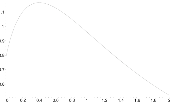
Figure 2: Evolution of the growing mode for the density contrast when $c=4$. For mathematical convenience we take $w=2$.

and for $c=10$ by

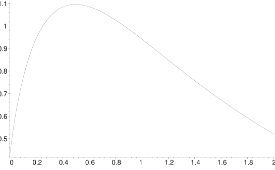
Figure 3: Evolution of the growing mode for the density contrast when $c=10$. For mathematical convenience we take $w=2$.

5 The reach of the non linear regime for the density contrast

In order to evaluate the time for the perturbation to reach the non-linear regime for the density contrast in our model, we use the Sachs-Wolf relation together with equation (48). Thus

$$\frac{\delta T}{T}\propto\frac{\delta\rho}{\rho}$$ (48)

is applicable for the considered models.

It is known that [20]

$$(\frac{\delta\rho}{\rho})_{dec}\leq O(10^{-2}-10^{-3}).$$ (49)

If we insert these values in our model, that is, in expression (48) one gets for $\tau$ the following

$$\tau_{dec}\sim O(10^{-4}-10^{-5})\,,$$ (50)

where $\tau_{dec}$ corresponds to the parameter at the decoupling time.

It seems reasonable to suppose that the present strong condensations grew out of small disturbances so that a necessary (if perhaps not sufficient) condition for their formation is that the perturbation, $\delta_{+}$ , calculated in linear stability should have become of order unity at some time before the present [21].

Consequently $\delta_{+}\sim 1$ implies that

$$\tau_{RL}\sim 10^{-1}$$ (51)

in our model.

We construct the quocient

$$Q=\frac{\tau_{RL}}{\tau_{dec}}=\frac{t_{RL}}{t_{dec}}\,$$ (52)

for to determinate the time for the perturbations reach the non linear regime ($t_{RL}$). Using (53) and (54) we obtain

$$Q=\frac{\tau_{RL}}{\tau_{dec}}\sim O(10^{3}-10^{4})\,.$$ (53)

If we insert these values into (54) and take in account that the decoupling occurred at $t\sim 10^{6}ys$ one finds

$$t_{RL}\sim O(10^{9}-10^{10})\,.$$ (54)

6 The horizon problem

Another crucial problem is to verify the horizon problem for Prigogine’s model. To this end, one should point out the distinction between the cosmological particle horizon and the Hubble sphere, or speed of light sphere, $R_{c}$, which is simply defined to be the distance from $\bf{O}$ of an object moving with the cosmological expansion and the velocity of light with respect to $\bf{O}$ . This can be seen very easily to be

$$R_{c}=\frac{R}{\dot{R}}=\frac{3}{4}\{\frac{1+c(e^{2\tau}-1)}{ce^{2\tau}}\}\,\,.$$ (55)

The cosmological particle horizon at time $t$ is given by

$$R_{H}=R(t)\int_{0}^{t}{R(t^{{}^{\prime}})^{-1}dt^{{}^{\prime}}}\,\,.$$ (56)

For our model, this is given by

$$R_{H} = \frac{1}{4}(b-U)^{\frac{2}{3}}[\ln{\frac{(U^{\frac{1}{3}}+b^{\frac{1}{3}})(1-b^{\frac{1}{3}}+b^{\frac{2}{3}})}{(U^{\frac{2}{3}}-(bU)^{\frac{1}{3}}+b^{\frac{2}{3}})(1+b^{\frac{1}{3}})^{2}}}-2\sqrt{3}\arctan{\frac{\sqrt{3}}{3}(\frac{-2U^{\frac{1}{3}}+b^{\frac{1}{3}}}{b^{\frac{1}{3}}})}+$$ (57)

$$+ 2\sqrt{3}\arctan{\frac{\sqrt{3}}{3}(\frac{b^{\frac{1}{3}}-2}{b^{\frac{1}{3}}})}\,.$$

$U$ is given by (36), $b=c-1$ and c is given by (14). Due to the analytical difficulties of comparing $R_{c}$ and $R_{H}$ we plot their graphs (fig.4). The horizon problem is solved when $c$ is large (that is when the initial number of particles per volume is large).

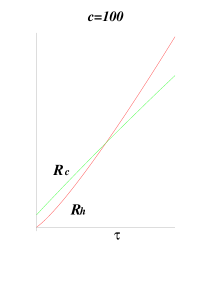
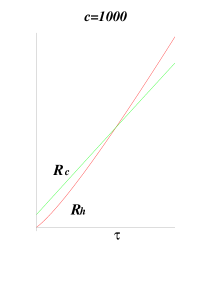
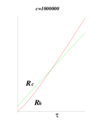
Figure 4: Cosmological particle horizon(red) and Hubble sphere(green) vs. $\tau$ for various values of $c$. The particle horizon intercept the Hubble sphere for: $c=2\rightarrow\tau\sim 0.38$; $c=4\rightarrow\tau\sim 0.27$; $c=10\rightarrow\tau\sim 0.16$; $c=100\rightarrow\tau\sim 3*10^{-2}$; $c=1000\rightarrow\tau\sim 3*10^{-3}$; $c=1000000\rightarrow\tau\sim 3*10^{-6}$   .

7 The Age of the universe

We now turn our attention to evaluate the characteristic time scale for the age of the universe with the ultimate aim of determining $t_{p}$, the time that elapsed from the beginning of the universe until now.

The recent results from the Cosmic Background Explorer (COBE) strongly supports the gravitational instability theory of structure formation and can be interpreted as providing evidence for the existence of small inhomogeneities generated in the early era. For the Priogogine’s model the perturbation is given by

$$\delta_{+}=\frac{R(t)}{e^{\beta t}}\,,$$ (58)

where

$$\beta=\frac{\alpha kM}{6}\,.$$ (59)

With the aid of equation (60) it can be written as

$$\frac{\delta_{+}(t_{p},\beta)}{\delta_{+}(t_{dec},\beta)}=(1+Z_{dec})e^{-\beta(t_{p}-t_{dec})}\,,$$ (60)

where $Z_{dec}$ is the decoupling redshift.

By assuming that during the matter dominated era particle production are restricted to non relativistic ones and its amplitude is fixed at decoupling time (COBE roughly fix this amplitude), we have

$$\frac{\delta_{+}(t_{p},\beta)}{\delta_{+}(t_{p},\beta=0)}=e^{-\beta(t_{p}-t_{dec})}=\frac{\sigma_{8}(\beta)}{\sigma_{8}(\beta=0)}$$ (61)

and

$$\delta_{+}(t_{dec},\beta)=\delta_{+}(t_{dec},\beta=0)\,,$$ (62)

where $\sigma_{8}(\rho)$ is the root-mean-square mass fluctuation in sphere of radius $8h^{-1}MPc$. The recent COBE measurements indicate that $\sigma_{8}(\beta=0)\sim 1$ for the standard cold dark matter [Liddle].

By requiring that structures form not to late, it is safe to assume $\sigma_{8}(\beta)\geq\frac{1}{3}$ [22]. Using this condition into equation (63) implies that

$$e^{-\beta(t_{p}-t_{dec})}\geq\frac{1}{3}\,.$$ (63)

If we assume that $t_{p}>>t_{dec}$, a superior limit for the age of the universe may be presented as

$$t_{p}\leq\frac{6.6}{\alpha kM}\,,$$ (64)

which becomes in term of the parameter $\tau$, using (49), as

$$\tau_{p}\leq 0.55\,.$$ (65)

In order to give a better idea on the superior limit of the age of the universe, we follow the same procedure used in the last section. We construct the quotient

$$\tilde{Q}=\frac{\tau_{p}}{\tau_{dec}}\,.$$ (66)

Fixing $\tau_{p}\sim 0.55$ and $\tau_{dec}\sim 10^{-4}-10^{-5}$, one gets

$$\tilde{Q}\sim O(10^{4}-10^{5})\,.$$ (67)

Once again if we take for the decoupling time $t_{p}\sim 10^{6}$ ys one has then

$$t_{p}\sim(10^{10}-10^{11})\,\,ys\,.$$ (68)

This result indicates that for the Prigogine’s model, the age of the universe is superior to the age of the structure formation and have an interval which agrees with the actual estimation.

8 Conclusions

In summary, in this paper we analyze the growth of density perturbation in Newtonian cosmological model for Prigogine’s type model to find a class of hypergeometric solutions.

A special case is studied to obtain an increasing and a decreasing mode analogous to Friedman model.

An estimate of the time interval for the perturbation to reach the non-linear regime is obtained.

An upper limit of the age of the universe is obtained by making use of Cobes’ data.

The horizon problem was carefully explained to show that for big values of the parameter $c$ the space-time is connected casually.

References

- [1] G.Gamow, Phys.Rev 74 , 505 (1948).
- [2] F.Hoyle, ApJ 118 , 513 (1953).
- [3] W.B.Bonnor, MNRAS 117 , 104 (1957).
- [4] G.B. van Albada, Bull. Astron. Inst. Netherlands 15 , 165 (1960).
- [5] G.B. van Albada, ApJ 66 , 590 (1961).
- [6] C.Hunter, ApJ 136 , 594 (1962).
- [7] M.P. Savedoff and S. Vila, ApJ 136 , 609 (1962).
- [8] D. Layzer, ApJ 137 , 351 (1963).
- [9] I.R. Gilbert, ApJ 144 , 233 (1966).
- [10] T.T. Arny, ApJ 145 , 572 (1966).
- [11] E.R. Harrison, Rev. Mod. Phys. 39 , 862 (1967).
- [12] M.de Campos and N.Tomimura, astro-ph/9911248 (1998).
- [13] I.Prigogine, J.Geheniau, E. Gunzig and P. Nardone, GRG 21, 767 (1989).
- [14] Joshua A. Frieman, astro-ph/9404040 (1994)
- [15] A. G.Riess et al, Astrop. J. 116, 1009 (1998).
- [16] S.Pelmuter et al.,preprint astro-ph/912473/9812133
- [17] L.R.W. Abramo and J.A.S.Lima, Class. Quantum Grav. 13(1996) 2953.
- [18] R. C. Arcuri and I. Waga, Phys. Rev. D 50, 2928 (1996)
- [19] P.J.E. Peebles, (Princeton University Press, Princeton, 1980)
- [20] E.W.Kolb and M.S. Turner, (Addison-Wesley, Redwood City, California, 1990)
- [21] S.Weinberg., Gravitation and Cosmology: Principles and Applications of the General Theory of Relativity (Jonh Wiley & Sons, New York, 1972)
- [22] A.R.Liddle and D.H.Lyth, Phys. Rep.231 ,1, (1993)