The Effect of the Outer Lindblad Resonance of the Galactic Bar
on the Local Stellar Velocity Distribution

Abstract

Hydro-dynamical modeling of the inner Galaxy suggest that the radius of the outer Lindblad resonance (OLR) of the Galactic bar lies in the vicinity of the Sun. How does this resonance affect the distribution function in the outer parts of a barred disk, and can we identify any effect of the resonance in the velocity distribution actually observed in the solar neighborhood? To answer these questions, detailed simulations of the velocity distribution, $f(\mbox{\boldmath$v$})$, in the outer parts of an exponential stellar disk with nearly flat rotation curve and a rotating central bar have been performed. For a model resembling the old stellar disk, the OLR causes a distinct feature in $f(\mbox{\boldmath$v$})$ over a significant fraction of the outer disk. For positions up to 2 kpc outside the OLR radius and at bar angles of $\sim$10-70 degrees, this feature takes the form of a bi-modality between the dominant mode of low-velocity stars centred on the local standard of rest (LSR) and a secondary mode of stars predominantly moving outward and rotating more slowly than the LSR.

Such a bi-modality is indeed present in $f(\mbox{\boldmath$v$})$ inferred from the Hipparcos data for late-type stars in the solar neighborhood. If one interpretes this observed bi-modality as induced by the OLR – and there are hardly any viable alternatives – then one is forced to deduce that the OLR radius is slightly smaller than $R_{0}$. Moreover, by a quantitative comparison of the observed with the simulated distributions one finds that the pattern speed of the bar is $1.85\pm 0.15$ times the local circular frequency, where the error is dominated by the uncertainty in bar angle and local circular speed.

Also other, less prominent but still significant, features in the observed $f(\mbox{\boldmath$v$})$ resemble properties of the simulated velocity distributions, in particular a ripple caused by orbits trapped in the outer 1:1 resonance.

1 INTRODUCTION

The fact that the Milky Way is barred has been established first of all by the interpretation of the gas velocities observed in the inner Galaxy ([de Vaucouleurs 1964]; [Peters 1975]; [Cohen & Few 1976]; [Liszt & Burton 1980]; [Gerhard & Vietri 1986]; [Mulder & Liem 1986]; [Binney et al. 1991]) and later confirmed by infrared photometry ([Blitz & Spergel 1991]; [Weiland et al. 1994]; [Dwek et al. 1995]; [Binney, Gerhard & Spergel 1997]) and asymmetries in the distribution or magnitude of stars ([Nakada et al. 1991]; [Whitelock & Catchpole 1992]; [Weinberg 1992]; [Nikolaev & Weinberg 1997]; [Stanek 1995]; [Sevenster 1996]; [Stanek et al. 1997]). However, there is still substantial debate on the structure and morphology of the bar, its orientation with respect to the Sun, and the rotation rate, usually referred to as pattern speed. Recent hydro-dynamical investigations of Englmaier & Gerhard (1999) and Weiner & Sellwood (1999) and the combined stellar- and gas-dynamical models of Fux (1999a) suggest that the bar rotates fast, i.e. that corotation occurs somewhere between 3.5 and 5 kpc (for $R_{0}=8\mbox{\,kpc}$) not much beyond the end of the bar. Moreover, the bar angle, the azimuth of the Sun with respect to the bar’s major axis, is restricted both by photometry and kinematics to lie in the range between about $10^{\circ}$ and $45^{\circ}$.

Apart from the corotation resonance (CR), a rotating bi-symmetric bar creates two other fundamental resonances, the inner (ILR) and outer (OLR) Lindblad resonances, which occur when

$$\Omega_{\rm b}=\omega_{\phi}\mp\case{1}{2}\omega_{R}.$$ (1)

Here, $\omega_{\phi}$ and $\omega_{R}$ are the azimuthal and radial orbital frequencies, while $\Omega_{\rm b}$ is the pattern speed of the bar. An orbit for which relation (1) is satisfied is in phase with the bar, i.e. after each completion of one radial lobe the orbit is at the same position with respect to the bar. Thus, a star on a resonant orbit is always pushed in the same direction, and thus forced into another orbit.

For circular orbits, $\omega_{\phi}=\Omega(R)$ (circular frequency) and $\omega_{R}=\kappa(R)$ (epicycle frequency) and each resonance can be mapped uniquely to the radius of the resonant circular orbit; hereafter $R_{\rm\scriptscriptstyle OLR}$ and $R_{\rm\scriptscriptstyle CR}$ denote the radii where circular orbits are in outer Lindblad and corotation resonance. For a nearly flat Galactic rotation curve, $R_{\rm\scriptscriptstyle OLR}\approx 1.7R_{\rm\scriptscriptstyle CR}$ and, from the aforementioned estimates for $R_{\rm\scriptscriptstyle CR}$, we find $R_{\rm\scriptscriptstyle OLR}\sim 6$-9 kpc. Thus, we expect the OLR of the Galactic bar to be located in our immediate Galactic surrounding. The goal of this paper is to answer the question whether and how this proximity of the resonance affects the stellar kinematics observable in the solar neighborhood.

Stellar Dynamics Near the OLR

Using linear perturbation theory for near-circular orbits (cf. Binney & Tremaine 1987, p. 146-151), one finds that closed orbits in a barred potential are elongated either parallel or perpendicular to the bar. The orientation changes at each of the fundamental resonances: inside ILR orbits are anti-aligned (so-called x₂ orbits), between the ILR and CR they are aligned (x₁ orbits), while between CR and OLR the orbits are anti-aligned, until they align again beyond the OLR.

fig:olr

Figure 1: Closed orbits (solid) just inside and outside the OLR of a rotating central bar (shaded ellipse). The circles (dotted) depict the positions of the ILR, CR, and OLR (from inside out) for circular orbits. Note the change of the orbits’ orientation at the OLR, resulting in the crossing of closed orbits at four azimuths. A possible position of the Sun is shown as filled circle. The bar angle $\phi$ is indicated for the case of a clockwise rotating bar.

The situation at the OLR is sketched in Figure 1, which shows two closed orbits (solid curves) just in- and outside the OLR as they appear in a frame of reference corotating with the bar. In this frame, the orbits near OLR rotate counter-clockwise for a clockwise rotating bar, like that of the Milky Way. Thus, at bar angles $\phi$ between $0^{\circ}$ and $90^{\circ}$, the closed orbits inside OLR move slightly outwards, while those outside OLR move inwards. Clearly, if all disk stars moved on closed orbits, the stellar kinematics would deviate from that of a non-barred galaxy only at positions very close to $R_{\rm\scriptscriptstyle OLR}$, where the closed orbits are significantly non-circular. In particular, at azimuths where the closed orbits from either side of the OLR cross, one would expect two stellar streams, one moving inwards and the other outwards.

However, in general stellar orbits are not closed, but exhibit radial oscillations. Many of these orbits are trapped into resonance ([Weinberg 1994]), and may be described, to lowest order in their eccentricity, as epicyclic oscillations around a closed parent orbit. This means in particular, that such trapped eccentric orbits from inside the OLR, i.e. with $\Omega_{\rm b}<\omega_{\phi}+\case{1}{2}\omega_{R}$, can visit locations outside $R_{\rm\scriptscriptstyle OLR}$, and vice versa. Thus, the stellar velocity distribution observable in the solar neighborhood, $f_{0}(\mbox{\boldmath$v$})$, shall be affected by the OLR whenever near-resonant orbits pass near the Sun and are sufficiently populated. We may estimate, using the epicycle approximation in a back-of-the-envelope calculation, that for late-type disk stars this condition is satisfied for $R_{\rm\scriptscriptstyle OLR}$ in the range from 6 to 9 kpc (for $R_{0}=8\mbox{\,kpc}$). This coincides with the above estimate for $R_{\rm\scriptscriptstyle OLR}$. Thus, we expect the OLR of the Galactic bar to affect the velocity distribution observable locally for late-type stars. Based on the properties of the closed orbits, one would expect also for stars moving on non-closed orbits different typical velocities depending whether they originate from in- or outside the OLR. Thus, the expected effect on $f_{0}(\mbox{\boldmath$v$})$ is a bi-modality.

Weinberg (1994) has studied the orbital response to a rotating bar using epicycle theory and assuming a flat rotation curve. He found indeed that different orbital families may overlap creating a bi-modality in the velocity distribution (though he only considered the resulting increase in the velocity dispersions). Weinberg also considered a slowly decreasing pattern speed, which affects the relative number of stars trapped into resonance with the bar, but leaves the final phase-space position of the resonance, and hence the velocity of possible modes in $f_{0}(\mbox{\boldmath$v$})$, unchanged.

In order to verify and quantify these estimates and expectations of the response of a warm stellar disk to a stirring bar and its OLR, I performed numerical simulations, presented in Section 2. In Section 3, I discuss the closed orbits in the outer part of a barred disk galaxy and their relation to the features apparent in the local $f(\mbox{\boldmath$v$})$, while Section 4 gives quantative estimates for the velocity of the secondary mode induced by the OLR. In Section 5, the velocity distribution observed in the solar neighborhood, which indeed shows a bi-modality, is compared both qualitatively and quantitatively to those emerging from the simulations. Finally, Section 6 concludes and sums up.

Throughout this paper, I will use units of kpc and km s^-1 for radii and velocities, while frequencies and proper motions are given in km s^-1 kpc^-1.

2 THE SIMULATIONS

In order to investigate the typical structure of a dynamically warm stellar disk in the presence of a rotating bar, we simulate the slow growth of a central bar with constant rotation frequency in an initially axisymmetric equilibrium representing a warm stellar disk. Clearly, this does not simulate the true evolution of the Galaxy, since the stellar disk was hardly dynamically warm already when the bar formed. Moreover, the bar has presumably developed too, both in strength and in pattern speed. However, we are not aiming at simulating the formation of the Milky Way, but at answering the question for the effect of the OLR, which significantly alters the phase-space structure, independently of the formation history of the Galaxy.

2.1 The Simulation Technique

Currently, traditional $N$-body simulations are not suitable for studying the influence of the central bar on a stellar disk at high resolution: the required number of particles exceeds $10^{8}$ already for merely two-dimensional simulations, which makes them very CPU-time intensive and aggravates any investigation of the parameter space. However, $N$-body simulations are unnecessary luxury, as they provide dynamical self-consistency and model the whole system, both of which is not required in this study. Instead, we (i) assume the growth of a central bar, rather than simulate a bar-instability self-consistently, and (ii) only integrate trajectories which are crucial to the local velocity distribution, rather than those for the whole system. Moreover, Poisson noise is avoided by placing the trajectories on a regular grid in the observables and integrate backward in time (see Section 2.1.3 for details).

This technique, which may be called backward integrating restricted $N$-body method, is similar in spirit to that used in the method of perturbation particles ([Leeuwin, Combes & Binney 1993]), and has first been used by Vauterin & Dejonghe (1997, 1998), who studied the non-linear evolution of the stellar distribution function (DF) in the inner parts of a bar-unstable model, whereby using the analytic potential due to the dominant linear bar mode.

Because we are only interested in the effects on the planar motions in the outer disk, our modeling is two-dimensional, and we do not care much about the details of the inner Galaxy.

2.1.1 The Initial Equilibrium

Since we are interested only in near-circular trajectories passing through a point in the outer parts of the disk, a possible inadequateness of our model potential in describing the inner parts of the Galaxy is unimportant. Therefore, we take a simple power-law rotation curve

$$v_{\rm c}=v_{0}\,(R/R_{0})^{\beta}$$ (2)

as our initial axisymmetric model. Here, $R_{0}$ denotes the Sun’s distance from the Galactic center and $v_{0}$ the local circular speed. The corresponding underlying potential,

$$\Phi_{0}(R)=v_{0}^{2}\times\left\{\begin{array}[]{l@{$\quad$}l}\displaystyle(2\beta)^{-1}\,(R/R_{0})^{2\beta}&{\rm for\;}\beta\neq 0\\[4.30554pt] \displaystyle\ln(R/R_{0})&{\rm for\;}\beta=0,\end{array}\right.$$ (3)

is meant to originate partly from the gaseous and stellar components (disk, bulge/bar, halo) and partly from dark matter. In restricting our model to two dimensions, we make no assumptions about the vertical distribution of the matter generating the potential (3).

The dynamical equilibrium of the stellar disk is described by a simple DF, $f=F(E,L_{z})$, which depends on energy $E$ and angular momentum $L_{z}$ of the stars, and is given by equation (10) of Dehnen (1999b). The parameters of the DF are set such that it generates, to very good approximation, an exponential disk with scale length $R_{s}$ and an exponential velocity-dispersion profile with scale length $R_{\sigma}$ and local radial velocity dispersion $\sigma_{0}\equiv\sigma_{R}(R_{0})$.

2.1.2 The Bar Potential

The contribution of the bar to the potential in the outer disk is dominated by the quadrupole, and we neglect higher-order multipoles for simplicity. Some orbits visiting the outer disk may have passed through the inner disk and bar region. Therefore, we will use a slightly more elaborate model for the bar potential than that resulting from just a constant quadrupole moment:

$$\Phi_{\rm b}=A_{\rm b}\,\cos\left(2[\phi-\Omega_{\rm b}t]\right)\,\times\left\{\begin{array}[]{l@{$\quad$}l}-(R_{\rm b}/R)^{3}&{\rm if}\;R\geq R_{\rm b},\\[8.61108pt] (R/R_{\rm b})^{3}-2&{\rm if}\;R\leq R_{\rm b},\end{array}\right.$$ (4)

where $R_{\rm b}$ and $\Omega_{\rm b}$ are the size and pattern speed of the bar. The amplitude $A_{\rm b}$ of the quadrupole is switched on smoothly. It is zero before $t=0$, grows with time at $0<t<t_{1}$ as

$$A_{\rm b}=A_{\rm f}\left({3\over 16}\xi^{5}-{5\over 8}\xi^{3}+{15\over 16}\xi+{1\over 2}\right),\quad\xi\equiv 2{t\over t_{1}}-1,$$ (5)

and stays constant at $A_{\rm b}=A_{\rm f}$ after $t_{1}$. Thus, the amplitude and its first and second time derivative behave continuously for all $t$, guaranteeing a smooth transition from the non-barred to the barred state.

2.1.3 The Time Integration

The collisionless Boltzmann equation tells us that the DF remains constant along stellar trajectories. Thus, the value $f(\mbox{\boldmath$w$},t_{2})$ of the DF at some phase-space point $\mbox{\boldmath$w$}\equiv(\mbox{\boldmath$x$},\mbox{\boldmath$v$})$ and time $t_{2}$ is equal to $f(\mbox{\boldmath$w$}_{0},0)$ if $w$ originates from integrating $\mbox{\boldmath$w$}_{0}$ from $t=0$ to $t=t_{2}$. In our case and in contrast to $N$-body simulations, the potential as function of space and time is known a priori. Therefore, we can obtain $\mbox{\boldmath$w$}_{0}$ just by integrating the orbit passing through $w$ at $t_{2}$ backward in time until $t=0$.

In practice, we specify the final time $t_{2}$ and choose the phase-space points $w$ from a grid in planar velocities at a position $(R_{0},\phi)$ in the Galactic plane. Each of the resulting orbits is integrated backward until $t=0$, and the initial energy $E$ and angular momentum $L_{z}$ are remembered. From these, the value $f(\mbox{\boldmath$w$},t_{2})=f(\mbox{\boldmath$w$}_{0},0)\equiv F(E,L_{z})$ can be computed for any initially axisymmetric equilibrium DF $F$.

2.2 The Parameters

Some of the parameters arising in the simulations are unimportant for our purposes. For instance, the size $R_{\rm b}$ of the bar, which, in agreement with the findings mentioned in Section 1, we fix to be 80% of the corotation radius. For our model, the latter is given by

$$R_{\rm\scriptscriptstyle CR}\equiv R_{0}\,(\Omega_{\rm b}/\Omega_{0})^{1/(\beta-1)},$$ (6)

where $\Omega_{0}\equiv v_{0}/R_{0}$ denotes the local circular frequency.

Since our simulations are not self-consistent, the parameters of the DF are unimportant for the dynamics of the stellar orbits, but crucial for their population with stars. In this study, we will use a DF designed to resemble the old stellar disk. The exponential surface density has scale length $R_{s}=0.33R_{0}$, the exponential velocity dispersion is normalized to $\sigma_{R}(R_{0})=0.2v_{0}$ and has scale length $R_{\sigma}=R_{0}$. I also experimented with $R_{\sigma}=0.66R_{0}$, corresponding to $\sigma_{R}^{2}\propto\Sigma$, and found very similar results.

2.2.1 The Time Scales

It turns out that the time $t_{1}$, determining how smoothly the bar is switched on, is not very important for the outcome of the simulations. However, the total integration time under influence of the bar, i.e. $\approx t_{2}-t_{1}/2$, has a significant impact on the details of the resulting velocity distributions. We will use $t_{2}=2t_{1}$ and consider various values for $t_{1}$ in units of the bar rotation period $T_{\rm b}\equiv 2\pi/\Omega_{\rm b}$.

2.2.2 The Solar Position

The relative distance of the Sun from the bar is conviently parametrized by the ratio $R_{\rm\scriptscriptstyle OLR}/R_{0}$, where for the power-law models (2.1.1)

$$R_{\rm\scriptscriptstyle OLR}=R_{0}\left({\Omega_{0}\over\Omega_{\rm b}}\,\left[1+\sqrt{1+\beta\over 2}\right]\right)^{1/(1-\beta)}.$$ (7)

Another important parameter is the bar angle $\phi$, the angle by which the Sun is behind the bar’s major axis (cf. Fig. 1).

2.2.3 The Rotation Curve

The shape of the rotation curve, parametrized by the power $\beta$ (see equation [2]), dictates the energy dependence of the orbital frequencies. We use a flat rotation curve ($\beta=0$) as default but will also consider slightly rising or falling rotation curves.

Changing the local circular speed $v_{0}$, or equivalently the frequency $\Omega_{0}$, at fixed $R_{\rm\scriptscriptstyle OLR}/R_{0}$ corresponds to a change of the pattern speed $\Omega_{\rm b}$ by the same factor. Such a change is essentially a re-scaling of the model and does not require any additional simulations.

2.2.4 The Bar Strength

The strength of the bar is best measured in a way that is independent of such re-scaling. We will use as parameter the dimensionless quantity

$$\alpha\equiv 3\,{A_{\rm f}\over v_{0}^{2}}\,\left({R_{\rm b}\over R_{0}}\right)^{3},$$ (8)

which is the ratio of the forces due to the bar’s quadrupole and the axisymmetric power-law background at galactocentric radius $R_{0}$ on the bar’s major axis.

2.3 Scanning the Parameter Space

Simulations have been performed for $R_{\rm\scriptscriptstyle OLR}/R_{0}$ between 0.8 and 1.2 at steps of 0.05, nine values of $\beta$ at steps of $0.05$ between $-0.2$ and $0.2$, and bar angles $\phi$ at $5^{\circ}$ intervals between $10^{\circ}$ and $50^{\circ}$. Additionally, the integration time and bar strength have been varied. In the figures below, unless stated otherwise, all the parameters but one are fixed to the default values listed in Table 2.3, in order to show the effect of one parameter alone. These default parameters correspond to an OLR less than 1 kpc inside the solar circle, a bar angle of 25^∘ as discussed from studies of the gas motions, and a flat rotation curve.

In order to ease a comparison with the observations, the velocity distributions arising from the simulations are displayed in the $u$ and $v$, defined, respectively, as the velocity towards the Galactic center and in direction of rotation, both relative to the circular orbit passing through the position of the Sun in absence of any bar.

tab:default

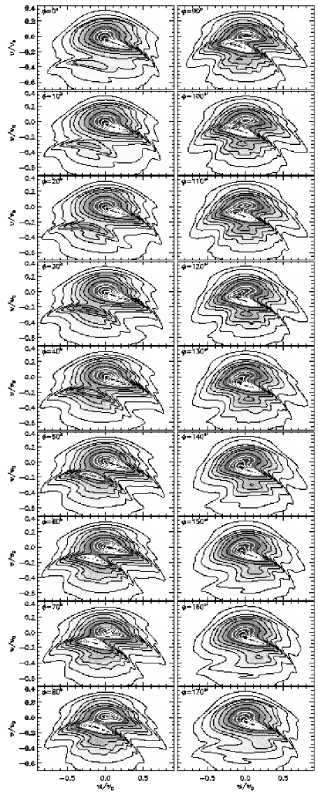
Figure 2: Simulated velocity distributions $f_{0}(u,v)$: variation with bar angle. The remaining parameters are fixed at their default values in Table 2.3.

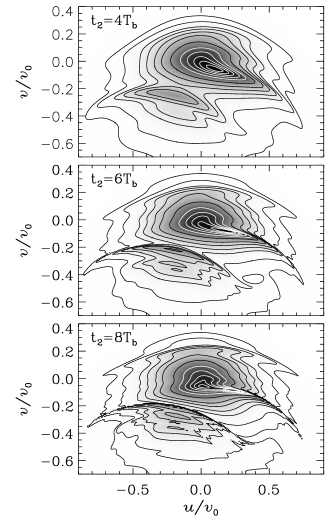
Figure 3: Simulated velocity distributions $f_{0}(u,v)$: variation with integration time $t_{2}$ ($T_{b}$ denotes the bar rotation period). The bar-growth time is set to $t_{1}=0.5t_{2}$.

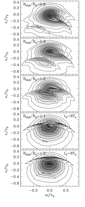
Figure 4: Simulated velocity distributions $f_{0}(u,v)$: variation with $R_{\rm\scriptscriptstyle OLR}/R_{0}$.

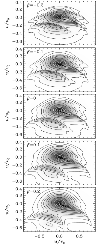
Figure 5: Simulated velocity distributions $f_{0}(u,v)$: variation with $\beta$, parameterizing the shape of the rotation curve.

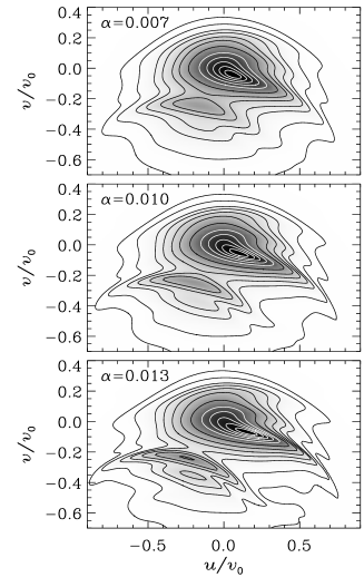
Figure 6: Simulated velocity distributions $f_{0}(u,v)$: variation with bar strength, parameterized by $\alpha$.

Table 1

Default values for the simulation parameters parameters to be varied default value shape of rotation curve $\beta$ 0 bar angle $\phi$ 25 $\!\!{}^{\circ}$ position w.r.t. OLR $R_{\rm\scriptscriptstyle OLR}/R_{0}$ 0 . 9 bar strength $\alpha$ 0 . 01 integration time $t_{2}$ 4 $T_{\rm b}$ parameters kept fixed default value bar size $R_{\rm b}/R_{\rm\scriptscriptstyle CR}$ 0 . 8 disk scale length $R_{s}/R_{0}$ 0 . 33 local velocity dispersion $\sigma_{R}(R_{0})/v_{0}$ 0 . 2 $\sigma_{R}$ scale length $R_{\sigma}/R_{0}$ 1 bar growth time $t_{1}$ 0 . 5 $t_{2}$

2.3.1 Variations with Bar Angle

Figure 2 plots $f_{0}(u,v)$ at intervals of $10^{\circ}$ in $\phi$ (note that the situation is bi-symmetric, so that $\phi$ and $\phi+180^{\circ}$ are identical) after the growth of a central bar. A bi-modality is clearly visible for bar angles in the first quadrant. As judged from these simulations, the existence of the bi-modality in $f_{0}$ seems not to depend critically on the bar angle.

When increasing the bar angle, the depression between the two modes, hereafter ‘LSR mode’ (at $\mbox{\boldmath$v$}\sim 0$) and ‘OLR mode’ (at $u,v<0$), is shifted towards higher $v$, while the OLR mode, which consists of stars originating from inside the OLR, becomes more prominent. However, the latter effect is hard to compare quantitatively with the observed $f_{0}(u,v)$, because the relative strength of the modes is likely to be affected both by the parameters of the DF and changes of the bar’s pattern speed during the past ([Weinberg 1994]). In $u$, the OLR mode ranges from about $-0.6$ to 0.2 in units of $v_{0}$.

There is also a clear distortion of the LSR mode, which, for bar angles relevant to our position in the Milky Way, has the form of an extension to positive $u$ velocities at $v$ comparable to that of the OLR mode.

2.3.2 Variations with Integration Time

Figure 3 plots $f_{0}(u,v)$ for three different choices of $t_{2}$ (with $t_{1}=0.5t_{2}$). Obviously, the longer integration times lead to more prominent resonant features, not only due to the OLR but also the resonance $\Omega_{\rm b}=\omega_{\phi}+\omega_{R}$, which is responsible for the ripple at $v_{0}\approx 0.2$. Clearly, the longer the action of non-axisymmetric forces, the stronger their imprints and the more detailed the resulting structures in stellar velocities. Other effects of longer integration times are a slight shift of the peak $v$ velocity of the OLR mode towards lower values and a change in the structure of the LSR mode. However, the velocity of the minimum between the two modes hardly changes, justifying the use of $t_{2}=4T_{b}$ as default.

These simulations, assuming a constant pattern speed and a completely flat rotation curve without any substructures like spiral arms, will certainly create much more such fine resonant features in $f_{0}(u,v)$ than the more noisy and less constant force field of a real galaxy would produce. However, the locus of the resonance itself is not such a detail and we can safely assume that the $v$-velocity of the division line between the modes is not subject to artefacts due to the idealizations made.

2.3.3 Variations with Radius

Figure 4 plots $f_{0}(u,v)$ for five different choices of the observers distance from the OLR, where for $R_{\rm\scriptscriptstyle OLR}/R_{0}=1.1$ and 1.2, the integration time is taken to be $t_{1}=8T_{b}$ in order to strengthen any possible resonant features. The bi-modality is clearly visible at $0.8\ga R_{\rm\scriptscriptstyle OLR}/R_{0}\ga 1.05$ – note, however, that this ‘visibility’ depends on the parameters of the DF and the bar angle $\phi$, cf. Fig. 2.

For $R_{\rm\scriptscriptstyle OLR}/R_{0}\ga 1.05$, the OLR does not create a clear bi-modality (at least not at $\phi=25^{\circ}$) but a distortion in $f_{0}(u,v)$ in form of a ripple at roughly constant energy (curves of constant energy in the $uv$ plane are circles centred on $u=0$, $v=-v_{0}$). For $R_{\rm\scriptscriptstyle OLR}/R_{0}=1.2$, most stars are on orbits between corotation and outer Lindblad resonance. Despite this proximity to two fundamental resonances, the resulting $f_{0}(u,v)$ is remarkably regular: apart from the ripple caused by the OLR, it forms a nice elliptical distribution (bottom panel of Fig. 4).

2.3.4 Variations with Rotation-Curve Shape

Figure 5 plots $f_{0}(u,v)$ for five different choices of $\beta$, which determines the shape of the rotation curve (2). Changing $\beta$ affects the orbital frequencies, in the sense that they fall off more steeply with energy for a falling rotation curve ($\beta<0$) than for a rising one ($\beta>0$). For a fixed difference in frequencies, a steeper fall-off results in a smaller energy difference, which at fixed position yields a smaller velocity distance. Therefore, reducing $\beta$ squashes the structures of the velocity distribution in $v$: the extent in $v$ of the OLR mode shrinks and its peak $v$ velocity becomes less negative (the opposite happens when increasing $\beta$). Similarly, the distance in $v$ between the OLR and higher-order resonances (responsible for the ripples at $v>0$) decreases with decreasing $\beta$

2.3.5 Variations with Bar Strength

Figure 6 plots $f_{0}(u,v)$ for three different bar strengths, parameterized by the force ratio $\alpha$ equation [8]. Apparently, stronger bars lead to more pronounced OLR (as well as other resonant) features in $f_{0}(u,v)$: the OLR mode contains more stars and extends over a larger range in $u$ velocity.

The $v$ velocity dividing the LSR and OLR modes is hardly changed. This is not what one would naively expect from linear theory, in which the amplitude of the orbital changes is proportional to the amplitude of the perturbation. However, large-amplitude orbital changes are not suitably described by linear theory, but result, in the case of the OLR, in orbits that are detuned by the non-linearity and thus leave the near-resonant region of phase space. Thus, the OLR mode is made from orbits which are shifted by similar amplitudes largely independent of the strength of the bar perturbation.

Figure 7: Characteristic diagram (plot of $R$ vs. $L$ on the bar’s minor axis) of the stable (solid) and unstable (dotted) closed orbits in the outer parts of the model with default settings. Orbits corresponding to high-order resonances ($n<-2$) are not displayed. The dashed line corresponds to the circular orbits in the unbarred model with the square indicating the OLR.

Figure 8: Closed orbits of the families also displayed in Fig. 7. The OLR is indicated by the bold circle. Solid and dotted curves refer to stable and unstable orbits, respectively. The x₁(1) orbits extend to larger radii, while for the other four orbital families the innermost and outermost orbit is shown (note the difference in scale). The 1:1 resonant orbits (d & e) also exist as reflected versions, such that each family as a whole is bi-symmetric.

3 RELATION TO CLOSED ORBITS

When a bar is slowly grown, the initially circular orbits will be mapped into (nearly) closed, but no longer circular, orbits in the barred potential. These are also the orbits on which gas is supposed to move, since encounters are avoided. Thus, we expect most stars in a barred galaxy to move on nearly closed orbits. Consequently, the properties of the velocity distributions are better understood in light of the properties of the closed orbits that exist in the outer parts of a barred disk.

3.1 Closed Orbits in the Outer Disks of Barred Galaxy

The only literature on this topic appears to be a review by Contopoulos & Grosbøl (1989), who consider closed orbits in the inner and outer parts of disks with bars or spiral structure.

Outside of corotation, the main family of closed orbits are the near-circular x₁ orbits. At each integer value of the rotation number

$$n={\omega_{R}\over\omega_{\phi}-\Omega_{\rm b}},$$ (9)

however, this family is modified by a resonance. At resonances with even $n$ (as e.g. the OLR, which has $n=-2$), this modification takes the form of a gap with a distinct change in properties, such as shape, between the orbits on either side of the resonance. At resonances with odd $n$, two families of orbits, one symmetric and one anti-symmetric with respect to the bar’s minor axis, branch off the main x₁ family. Immediately outside corotation, the denominator in equation (9) scans through all small negative numbers, resulting in a whole host of high-order resonances with $-\infty<n<-2$. Figure 7 shows the characteristics of the orbit families with $n\geq-2$ in the model with the default parameters of Section 2.

fig:char fig:orbits

At $n=-2$ (OLR) we have the typical change, already mentioned in the introduction, from orbits inside OLR, which anti-align with the bar and are called x₁(2) orbits by Contopoulos & Grosbøl, to orbits outside OLR, called x₁(1) and aligning with the bar. The first subfamiliy, x₁(2), extends to unstable orbits, called x${}_{1}^{\star}$(2), at larger radii. Some orbits of these families are shown in the upper three panels of Figure 8. The innermost x₁(2) orbit clearly shows the effect of the $n=-4$ resonance.

The resonance with $n=-1$, also called –1:1 or outer 1:1 resonance, creates a pair of orbit families (Fig. 8 d&e), each of which exists in two versions, which are reflection symmetric to each other. The family which is symmetric with respect to the bar’s minor axis consists of stable orbits, while the antisymmetric family contains only unstable orbits. At large radii, both these family develop inner loops, which may penetrate right into the central bar.

3.2 Closed Orbits and $f_{0}$

All of the orbital subfamilies in Figure 8 pass through positions with $R\sim R_{\rm\scriptscriptstyle OLR}$, but there is no position $(R,\phi)$ which is visited by orbits from all five families. Thus, the accessibility by closed and nearly closed orbits changes between different positions in the outer Galaxy. Since each stable family (and non-closed orbits trapped around it) will create a distinct feature in the velocity distribution, we expect that $f_{0}(u,v)$ changes almost discontinuously between different positions, depending on the closed orbits families passing through that position.

3.2.1 The Position $R_{\rm\scriptscriptstyle OLR}/R_{0}=0.9$ and $\phi=25^{\circ}$

Let us firts consider the case of the simulation with default parameters, cf. the middle panels of Figs. 5 and 6. There are three closed orbits reaching this position: two x₁(1) orbits and one x${}_{1}^{\star}$(2) orbit.

The first of the x₁(1) orbits has $(u,v)=(0.02,-0.015)v_{0}$, while for the second $(u,v)=(0.09,-0.1)v_{0}$. This latter orbit originates from very close to the OLR, resulting in a large pertubation, which enables its visit at $R_{0}$. Both these velocities lie within the LSR mode, but while the first is very close to the undisturbed circular orbit, the local velocity of the latter is related to the extension towards $u>0$. Thus, we can understand these extensions of the LSR modes as caused by stars on nearly closed, hence strongly populated, and nearly OL-resonant, hence highly disturbed, orbits.

The third orbit reaching $(R_{0},\phi)$ is unstable and has $(u,v)=(-0.38,-0.19)v_{0}$. This velocity is exactly in the valley between the two modes. Thus, it seems that this valley is caused by unstable, i.e. chaotic, orbits.

3.2.2 Varying the Radius

Let us now consider what happens if we change the distance from the OLR. For $0.7\la R_{\rm\scriptscriptstyle OLR}/R_{0}\la 1$, there is an unstable x${}_{1}^{\star}$(2) orbit passing through, and we therefore expect a depression (a valley or a truncation) in $f_{0}$.

For $R_{\rm\scriptscriptstyle OLR}/R_{0}\ga 1$ (the detailed value depends on $\phi$), there is a fundamental change, as then (i) no stable closed x₁(1) orbits passes through, but (ii) a stable x₁(2) instead of an unstable x${}_{1}^{\star}$(2) orbit. These two changes are certainly related to the rather abrupt change of the morphology of $f_{0}(u,v)$ apparent in Figure 4, from a clear bi-modality to a mere density enhancement at roughly constant energy.

3.2.3 Varying the Azimuth

If we change the bar angle $\phi$ at fixed $R_{\rm\scriptscriptstyle OLR}/R_{0}$, the families of closed orbit passing through $(R_{0},\phi)$ change as well. In particular for $R_{\rm\scriptscriptstyle OLR}/R_{0}\sim 1$, the stable x₁(2) orbits appear for $\phi\ga 40^{\circ}$, which in Fig. 2 leads to a stronger OLR mode for $\phi\sim 90^{\circ}$ than for $\phi\sim 0^{\circ}$.

On the other hand, when increasing $\phi$, the second stable x₁(1) orbits disappear with the consequence that the extension of the LSR modes towards $u>0$ weakens as one moves from the bar’s major axis to its minor axis in Fig. 2.

3.2.4 The Outer 1:1 Resonance

Even though the stable 1:1 resonant closed orbits do not pass through positions near the OLR with $|\phi|\la 40^{\circ}$, there is a clear resonant feature in the velocity distributions at these positions. Hence, this feature, which takes the form of a density enhancement at certain velocities, must be due to related non-closed resonant orbits. The density enhancement is likely caused by the intersection of the various orbits of this family at $0^{\circ}\la\phi\la 180^{\circ}$.

4 QUANTIVYING THE OLR FEATURE

In order to allow for a quantitative comparison of the OLR feature in the simulated $f_{0}(u,v)$ with the observations in the next section, we need to use a well-defined quantity that is easy to measure and likely to be stable under deviations from the idealized conditions assumed in the simulations. Here, I will only use the $v$-velocity of the saddle point between the LSR and OLR mode. This velocity, hereafter denoted $v_{\rm\scriptscriptstyle OLR}$, is essentially independent of the details of the stellar DF and even the strength of the bar.

4.1 An Axisymmetric Estimate

We may first neglect the effect of the bar potential and estimate the velocities (at $R_{0}$) of the orbits that would become exactly resonant in the presence of a bar with pattern speed $\Omega_{\rm b}$. For power-law potentials, the orbital frequencies are well approximated by the corresponding frequencies of the circular orbit with the same energy ([Dehnen 1999a]). Using this approximation and the relations for power-law potentials (cf. Appendix B of Dehnen 1999a) and neglecting terms ${\cal O}(\mbox{\boldmath$v$}^{3}/v_{0}^{3})$, we may estimate that the local velocities of orbits that are in OLR satisfy

$$v+{u^{2}\over 2v_{0}}\cong\tilde{v}_{\rm\scriptscriptstyle OLR}\equiv v_{0}\,{1+\beta\over 1-\beta}\left[1-{\Omega_{\rm b}/\Omega_{0}\over 1+\sqrt{(1+\beta)/2}}\right].$$ (10)

Thus, the local velocities of resonant orbits form a parabola whose maximal $v$ occurs at $u=0$ and depends on the distance from the OLR and the shape of the rotation curve. Note that the valleys between the two modes in the simulated $f_{0}(u,v)$ are actually nearly parabolic. They are, however, displaced from the $u=0$ axis and also in $v$. These displacements must be due to the quadrupole forces of the bar, neglected in the above estimate.

4.2 Quantifying the Local OLR Velocity

The value for the velocity $v_{\rm\scriptscriptstyle OLR}$ is sensitive mainly to four parameters: the bar angle $\phi$, the relative distance $R_{\rm\scriptscriptstyle OLR}/R_{0}$ of the OLR, the normalization $v_{0}$ of the rotation curve, and its shape, parameterized by $\beta$. The dependence on $v_{0}$ is a simple scaling, while that on the other three parameters is less trivial.

We might hope that the dependence on $R_{\rm\scriptscriptstyle OLR}/R_{0}$ and $\beta$ is already largely described by $\tilde{v}_{\rm\scriptscriptstyle OLR}$ defined in equation (10). Indeed, from plotting $v_{\rm\scriptscriptstyle OLR}$ at fixed bar angle versus $\tilde{v}_{\rm\scriptscriptstyle OLR}$, we find that to good accuracy the dependence on $R_{\rm\scriptscriptstyle OLR}/R_{0}$ and $\beta$ is described by a linear function of the form

$$v_{\rm\scriptscriptstyle OLR}\approx a\,\tilde{v}_{\rm\scriptscriptstyle OLR}-(b+c\,\beta)\,v_{0}.$$ (11)

For bar angles $\phi\in[15^{\circ},50^{\circ}]$, Table 4.2 lists the best-fit values for $a$, $b$, and $c$ obtained from fitting $v_{\rm\scriptscriptstyle OLR}$ for $R_{\rm\scriptscriptstyle OLR}/R_{0}$ in the range from 0.8 to 0.95. Note that the values for $b$ and $c$ are always small, i.e. $v_{\rm\scriptscriptstyle OLR}$ is largely given by $a\,\tilde{v}_{\rm\scriptscriptstyle OLR}$. The rms error made by this approximation is $0.0035v_{0}$, while the maximal error is $0.013v_{0}$ (occuring for $R_{\rm\scriptscriptstyle OLR}/R_{0}=0.95$, $\beta=0.2$, $\phi=15^{\circ}$).

tab:fit

Table 2

Best-fit values for $(a,b,c)$ in equation (11) $\phi$ $a$ $b$ $c$ 15^∘ 1.3549 0.0761 0.1362 20^∘ 1.2686 0.0642 0.1120 25^∘ 1.2003 0.0526 0.0892 30^∘ 1.1424 0.0406 0.0711 35^∘ 1.0895 0.0298 0.0538 40^∘ 1.0420 0.0200 0.0423 45^∘ 1.0012 0.0103 0.0316 50^∘ 0.9653 0.0012 0.0238

5 COMPARISON WITH THE OBSERVED
VELOCITY DISTRIBUTION

Figure 9 shows the distribution $f_{0}(u,v)$ for late-type stars in the solar neighborhood (note that the volume sampled by these stars corresponds to the size of the dot in Fig. 1 referring to a possible solar position). Here, the velocities $u$ and $v$ are relative to the local standard of rest (LSR) as measured by Dehnen & Binney (1998) from a sample of about 14 000 stars in the Hipparcos catalogue (ESA 1997). This sample was constructed to be essentially magnitude limited in order to avoid any kinematic biases. The distribution shown in Figure 9 has been inferred statistically ([Dehnen 1998]) from the tangential velocities of about 6000 late-type main-sequence stars ($B-V>0.6\,$mag) and giants in Dehnen & Binney’s sample.

The distribution $f_{0}(u,v)$ has been inferred by maximizing the log-likelihood plus some penalty function which measures the roughness of $f$ (see Dehnen 1998 for more details). The latter ensures a smooth distribution and suppresses the amplification of shot noise. Error estimates using the boot strap method (cf. [Press et al. 1992]) indicate that the contours have an uncertainty of about 0.3-3 km s^-1. The two outermost contours are affected by the way the smoothing is introduced, and hence are less reliable. All features discussed in this section are of high significance.

5.1 The OLR Induced Bi-Modality

The distribution in Figure 9 shows a lot of structures. One of the most obvious is the bi-modality between a low-velocity component centred on the LSR motion (solid ellipse) and an intermediate-velocity component at $v\la-30$ and predominantly negative $u$ (broken ellipse), which contains about a every sixth late-type star near the Sun. This clear bi-modality was, to the best of my knowledge, not known from pre-Hipparcos data; the corresponding mean outward motion of stars with $v\la-30$ was called ‘$u$-anomaly’. The bi-modality is hardly present in samples of early-type stars, which almost exclusively populate the moving groups (sub-peaks) in the low-velocity region ([Dehnen 1998]; [Chereul, Creze & Bienayme 1998]; [Asiain et al. 1999]; [Skuljan, Hearnshaw & Cottrell 1999]).

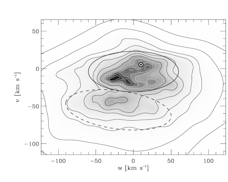
Figure 9: The velocity distribution $f_{0}(u,v)$ inferred from Hipparcos data for 3 527 main-sequence stars with $\bv\geq 0.6$ and 2 491 mainly late-type non-main-sequence stars, high-velocity stars excluded, in the solar neighborhood ([Dehnen 1998]). The symbol $\odot$ indicates the solar velocity. Samples of early-type stars contribute almost exclusively to the low-velocity region (solid ellipse), which contains the most prominent moving groups. The region of intermediate velocities (broken ellipse) is mainly represented by late-type stars, of which $\sim 15\%$ fall into this region. Gray scales are linear in $f_{0}$ and the contours contain, from inside out, 2, 6, 12, 21, 33, 50, 68, 80, 90, 95, 99, and 99.9 percent of all stars. The 1-$\sigma$ uncertainty in the contour lines is between 0.3 and 3 km s^-1.

5.1.1 Is the Bi-Modality due to the OLR?

The bi-modality present in the locally observed $f_{0}(u,v)$ (Fig. 9) is indeed very similar to those emerging from the simulations in Section 2. Moreover, since we expect, from our previous knowledge of the bar and its estimated pattern speed, that $R_{\rm\scriptscriptstyle OLR}\sim R_{0}$ (cf. Section 1), it is only natural to identify the observed bi-modality as the OLR feature of the Galactic bar. However, this may be premature to do and we must first check if there are viable alternative explanations.

First, can the intermediate-velocity mode at $v\approx-45$ be the relic of a dispersed stellar (open) cluster or association (the standard explanation for the formation of moving groups)? The strongest argument against this hypothesis comes from the age of the participating stars, which from the absence of early-type stars with intermediate velocities may be inferred to be $\ga 8$Gyr ([Dehnen 1998]). This high age, corresponding to $\ga 40$ orbital times, makes it very unlikely for any initial moving group to survive Galactic scattering processes. Moreover, the number of stars in the secondary mode is significantly higher than that in the low-velocity moving groups, such as the Hyades and Sirius streams.

Second, could this secondary mode be the result of a merger with a globular cluster or satellite galaxy? This again can be ruled out, since such a scenario is highly unlikely to produce a feature with disk-like kinematics (a velocity deviating from the LSR motion by only $\sim 15\%$ instead of an expected 100%; a vertical velocity distribution like that of low-velocity stars). Moreover, Raboud et al. (1998) have reported that the $u$-anomaly is caused by intermediate to high-metallicity stars, while a merger would involve rather metal poor stars.

Third, could the bi-modality be caused by any other, possibly resonant, scattering process, e.g. due to spiral arm structure? While this possibility is harder to exclude than the first two, it seems rather unlikely. Spiral structure should mainly affect stars with epicycles smaller than the inter-arm separation, while the bi-modality is created by stars with epicycles comparable or larger than 3 kpc. The possibility of inner Lindblad resonant scattering by some unknown agent corotating at $\sim 25\mbox{\,kpc}$, e.g. a slowly rotating halo or a satellite galaxy (note, however, that the magellanic clouds are too far out and have polar orbits, which disqualifies them as potential agents) was shown by Weinberg (1994) to be inconsistent with velocity dispersion data.

So, we can conclude that outer Lindblad resonant scattering off the Galactic bar is presently the only viable explanation that can explain the bi-modality observed in $f_{0}(u,v)$ of late-type disk stars and its absence in early-type stars.

Based on Fux’s (1997) $N$-body simulations of the Milky Way, Raboud et al. (1998) and Fux (1999b) also attributed the $u$-anomaly to the influence of the Galactic bar, but were unable to investigate the parameter space and to achieve a resolution, both spatially and in velocity, comparable to that in the observed distribution (a general problem with $N$-body simulations, see my remarks at the beginning of Section 2.1).

Figure 10: The ratio $\Omega_{\rm b}/\Omega_{0}$ that follows from the new constraint for given rotation curve parameters $v_{0}$, $\beta$, and bar angle $\phi$. The typical error in $\Omega_{\rm b}/\Omega_{0}$ due to the uncertainty in the measured $v_{\rm\scriptscriptstyle OLR}$ is about 1%, i.e. two small ticks on the $y$-axis. A small systematic error due to the $v$ motion of the LSR is likely to lead to an over-estimation of $\Omega_{\rm b}/\Omega_{0}$ by up to a few % for $\phi<45^{\circ}$ (see text).

5.1.2 Implications for the Inner Galaxy

A quick comparison with the simulations shows that (i) the OLR must be inside the solar circle, i.e. $R_{\rm\scriptscriptstyle OLR}<R_{0}$, and (ii) the bar angle $\phi$ in the range $10^{\circ}$ to $70^{\circ}$. We may even go further and make a quantitative comparison of the $v$-velocity

$$v_{\rm\scriptscriptstyle OLR}=(-31\pm 3)\mbox{\,km\,s${}^{-1}$},$$ (12)

of the valley between LSR and OLR mode with the corresponding velocity measured in the simulated $f_{0}(u,v)$. In Figure 10, the ratio of the bar’s pattern speed over the local circular frequency that is implied by the new constraint via the approximation (11) is plotted for various possible choices for the local run of the rotation curve (as given by $v_{0}$ and $\beta$) and the bar angle $\phi$.

fig:ObOz

The estimate in Fig. 10 is subject to some small systematic errors. In particular, while in the simulations $v_{\rm\scriptscriptstyle OLR}$ is defined relative to the circular speed $v_{0}$ in the absence of any bar, the value (12) obtained from the observed $f_{0}(u,v)$ has been measured relative to the LSR, which shall deviate from an exactly circular orbit. From the simulations, it is simple to estimate the size of this deviation caused by the bar itself (for which it is small, especially if $\phi\sim 45^{\circ}$), but this is not very meaningful as the LSR, being defined by low-eccentricity orbits, may well be affected by local spiral structure, not considered in the simulations. However, even if the azimuthal LSR motion as large as 10 km s^-1, it would introduce a systematic error of only by 3% for $\Omega_{\rm b}/\Omega_{0}$, i.e. an amount that is still smaller than the uncertainty due to the unknown bar angle $\phi$.

An IAU standard value of $v_{0}=220\mbox{\,km\,s${}^{-1}$}$ and a flat rotation curve yield $\Omega_{\rm b}$ between 1.8 and 1.9 times $\Omega_{0}$. When using the observed proper motion for the radio source Sgr A${}^{\!\star}$, which is thought to be associated with a supermassive black hole ([Eckart & Genzel 1997], [Ghez et al. 1998]), to constrain the value of the local circular frequency, one finds $\Omega_{0}\sim 28.5\mbox{\,km\,s${}^{-1}$\,kpc${}^{-1}$}$ ([Reid et al. 1999]; [Backer & Sramek 1999]), and thus $\Omega_{\rm b}\sim 51$ to $54\mbox{\,km\,s${}^{-1}$\,kpc${}^{-1}$}$.

See Dehnen (1999c) for a more detailled analysis of the consequences for the value of $\Omega_{\rm b}$, when additionally to the proper motion of Sgr A${}^{\!\star}$ the terminal gas velocities are used to constrain the run of the rotation curve. The main result from that study is that the value for $\Omega_{\rm b}$ depends only weakly on the assumed $R_{0}$ and $\phi$ (as long as they take reasonable values) and is thus rather narrowly constraint to be between 50 and 56 km s^-1 kpc^-1. Another result from that study is that corotation of the bar occurs at $R_{\rm\scriptscriptstyle CR}/R_{0}\approx 0.5$ to 0.6. This can be compared to the results from stellar- and hydro-dynamical modeling of the inner Galaxy: Weiner & Sellwood (1999) and Fux (1999a) report values in the same range, while Englmaier & Gerhard (1999) obtain an upper limit of $0.5$ for $R_{\rm\scriptscriptstyle CR}/R_{0}$, i.e. slightly discrepant with the new value.

5.2 More Similarities with the Simulations

Apart from the low- vs. intermediate-velocity bi-modality, the observed velocity distribution in Figure 9 has also other features in common with the distributions obtained in the simulations of Section 2.

5.2.1 The Structure of the LSR Mode

The structure of the main mode centred on the LSR, in particular the extension to $u>0$ at $v\approx-0.1v_{0}\sim-20\mbox{\,km\,s${}^{-1}$}$, is at least qualitatively similar, apart, of course, from the prominent moving groups. In the simulations, this extension is caused by stars on orbits that are nearly closed and have large perturbative amplitudes. These orbits originate from near the OLR and therefore have large deviations from circularity such that they may nonetheless visit the solar neighborhood.

However, since these orbits are nearly closed, they are liklely to be affected by spiral stucture and other local deviations from a smooth force field. As such effects have not been considered in the simulations of Section 2, it is not surprising that simulations and observations do not agree in detail.

5.2.2 Features due to the outer $1:1$ Resonance

The ripples at $(u,v)\approx(-80,-5)$ and $(40,5)$ are reminiscent of the ripples, for instance in Fig. 3, caused by the outer 1:1 resonance. This similarity persists even into details, which is more clearly recognizable when comparing to simulations with longer integration times, for instance, the middle panel of Fig. 3. Here, the $u<0$ side of the ripple is at smaller $v$ than the $u>0$ side, in agreement with the corresponding features in the observed $f_{0}(u,v)$. Moreover, there is a small excess of stars towards larger $v$ at $|u|<0.4v_{0}$, which may be compared to the ‘bump’ in the third and fourth contour (from outside) at $|u|<20\mbox{\,km\,s${}^{-1}$}$ and $v>20\mbox{\,km\,s${}^{-1}$}$ in Fig. 9. This bump is presumably caused by stars from outside the outer 1:1 resonance.

6 DISCUSSION AND CONCLUSION

The simulations presented in Section 2 showed how a rotating bar affects the distribution function of a surrounding stellar disk. Since the non-axisymmetric component of the bar-induced forces falls off steeply with radius ($\propto r^{-4}$ for the quadrupole) reaching about 1% of the total force at $R_{0}$, the influence of the bar is restricted to orbits which are nearly in resonance with it. This influence is strongest for the outer Lindblad resonance (OLR), which occurs for orbits whose radial and azimuthal frequencies obey the relation $\Omega_{\rm b}=\omega_{\phi}+\case{1}{2}\omega_{R}$, where $\Omega_{\rm b}$ is the bar’s rotation rate (pattern speed). At orbits that are nearly in OLR, an otherwise smooth stellar distribution function becomes distorted. At any given position in the disk, this distortion is visible in the observable stellar velocity distribution $f(u,v)$ if near-resonant orbits (i) pass through this position and (ii) are sufficiently populated. For a distribution function designed to resemble the old stellar disk of the Milky Way, the OLR leaves its imprint in the velocity distribution over a wide range of possible position in the disk.

For positions $(R_{0},\phi$) orientated relative to the bar at angles $\phi\in[10^{\circ},70^{\circ}]$ and situated outside the radius $R_{\rm\scriptscriptstyle OLR}$ where circular orbits are in OLR, the resulting feature in $f(u,v)$ is a clear bi-modality: apart from the dominant stellar component with velocities similar to the local standard of rest (LSR), there is a secondary mode at $u,v<0$. This OLR mode consists of stars with mean outward motion and slower rotation velocities than the LSR. For $R_{0}<R_{\rm\scriptscriptstyle OLR}$, the OLR induced feature occurs at higher rotation velocities than the LSR and no longer takes the form of a clear bi-modality. As has been demonstrated in Section 3, all these changes in the behaviour of $f_{0}(u,v)$ can be well understood from the properties of the closed orbits in the outer parts of a barred galaxy.

Extensive simulations showed that the precise velocity of the OLR-induced feature depends mainly on four parameters: the normalization and shape of the underlying circular speed curve, $v_{\rm c}(R)$, the observer’s relative position with respect to the OLR, $R_{\rm\scriptscriptstyle OLR}/R_{0}$, and their orientation relative to the bar, measured by the bar angle $\phi$. Note that the dependence on $v_{\rm c}(R)$ is restricted to its run in the region visited by near-resonant slightly eccentric orbits, i.e. between about $0.7R_{0}$ and $R_{0}$ for $R_{\rm\scriptscriptstyle OLR}=0.9R_{0}$. These dependences are such that the (negative) $v$-velocity, $v_{\rm\scriptscriptstyle OLR}$, separating the OLR mode from the LSR mode of $f_{0}$, increases (becomes smaller in modulus) with increasing bar angle $\phi$, decreasing ratio $R_{\rm\scriptscriptstyle OLR}/R_{0}$, $v_{0}\equiv v_{\rm c}(R_{0})$, and $\beta\equiv{\rm d}\ln v_{\rm c}/{\rm d}\ln R$.

The velocity distribution $f(u,v)$ actually observed for late-type stars in the solar neighborhood (Fig. 9) shows indeed a secondary mode at $u,v<0$, which is very similar to the OLR modes emerging in the simulations. As I have argued in Section 5.1.1, there exists no satisfying explanation of this seeming anomaly other than being the feature induced by the OLR of the Galactic bar. Interestingly, the observed $f_{0}(u,v)$ has also other features in common with the simulated distributions. Firstly, extensions towards high $u$ (inward moving) at slightly negative $v$ may be related to a ridge in Fig. 9 at $v\approx{-}20\mbox{\,km\,s${}^{-1}$}$ connecting the Hyades and Pleiades stream and reaching at least to $u\approx 60\mbox{\,km\,s${}^{-1}$}$. Secondly, ripples due to the outer 1:1 resonance seen in the simulated $f(u,v)$ at $v\geq 0$ and large $|u|$ may be related to the features in Fig. 9 at $(u,v)=(-80,-5)$ and $(40,5)\mbox{\,km\,s${}^{-1}$}$.

First of all, this means that the structure of the local velocity distrubution for late-type stars provides a clear evidence for the existence of the Galactic bar, completely independent of any observation of the inner Galaxy itself. Moreover, this structure implies that the Sun is situated slightly outside of the radius $R_{\rm\scriptscriptstyle OLR}$ and at bar angles $\phi$ between about $10^{\circ}$ and $70^{\circ}$. One may even use the observed value, $v_{\rm\scriptscriptstyle OLR}$, for the $v$-velocity seperating the OLR and LSR mode in order to deduce that the ratio between the bar’s pattern speed $\Omega_{\rm b}$ and the local circular speed $\Omega_{0}$ is between 1.75 and 2. The uncertainty here is dominated by the uncertainty in the bar angle $\phi$, which according to other evidence must lie somewhere in the range 20 to 45 degrees. Combining this result with the value $\Omega_{0}\approx 28.5\mbox{\,km\,s${}^{-1}$\,kpc${}^{-1}$}$ derived from the proper motion of the radio source Sgr A${}^{\!\star}$ at the Galactic centre ([Backer & Sramek 1999]; [Reid et al. 1999]) yields $\Omega_{\rm b}=(53\pm 3)\mbox{\,km\,s${}^{-1}$\,kpc${}^{-1}$}$.

Clearly, the conclusion on the precise value of $\Omega_{\rm b}$ drawn on the basis of the simulations of Section 2 is subject to (presumably small) systematic errors, originating from the simplifications made in the simulations and from the unknown $v$ motion of the LSR. To improve on this, one needs to (i) use a more realistic model for the Galactic potential, (ii) compare not only $v_{\rm\scriptscriptstyle OLR}$ of the simulated $f_{0}(u,v)$ but also the feature of the 1:1 resonance (to reduce systematic errors due to the unknown LSR azimuthal motion), and (iii) combine this with hydro-dynamical simulations, which can be compared directly to the gas velocities observed in the entire inner Galaxy, constraining both the bar parameters and the rotation curve. Such simulations, in conjunction with the constraint set by the proper motion of Sgr A${}^{\!\star}$, are likely to determine the pattern speed, orientation, and structure of the bar as well as the rotation curve and hence mass distribution of the inner Galaxy. In such an analysis, the constraints set by the local $f_{0}(u,v)$ constitute important new ingredients as they largely reduce the freedom for the pattern speed $\Omega_{\rm b}$, which is not very well constraint by modeling of the inner Galaxy as is apparent from the diverging results obtained in the past by different modellers.

Thus, the velocity distribution observed locally imposes important new constraints for the structure of the inner Galaxy independent of and complementary to the photometry and kinematics, both stellar and gaseous, of that region itself.