M31 Globular Clusters: Colors and Metallicities

Abstract

We present a new catalog of photometric and spectroscopic data on M31 globular clusters. The catalog includes new optical and near-infrared photometry for a substantial fraction of the 435 clusters and cluster candidates. We use these data to determine the reddening and intrinsic colors of individual clusters, and find that the extinction laws in the Galaxy and M31 are not significantly different. There are significant (up to $0.2^{m}$ in $V\!-\!K$) offsets between the clusters’ intrinsic colors and simple stellar population colors predicted by population synthesis models; we suggest that these are due to systematic errors in the models. The distributions of M31 clusters’ metallicities and metallicity-sensitive colors are bimodal, with peaks at ${\rm[Fe/H]}\approx-1.4$ and $-0.6$. The distribution of $V\!-\!I$ is often bimodal in elliptical galaxies’ globular cluster systems, but is not sensitive enough to metallicity to show bimodality in M31 and Galactic cluster systems. The radial distribution and kinematics of the two M31 metallicity groups imply that they are analogs of the Galactic ‘halo’ and ‘disk/bulge’ cluster systems. The globular clusters in M31 have a small radial metallicity gradient, suggesting that some dissipation occurred during the GCS formation. The lack of correlation between cluster luminosity and metallicity in M31 GCs shows that self-enrichment is not important in GC formation.

1 Introduction

The study of the Andromeda Galaxy (M31) has been, and continues to be, a keystone of extragalactic astronomy. The recognition of M31 as an external galaxy by Hubble marked the beginning of the field of extragalactic astronomy, and the recognition of Populations I and II in M31 by Baade began the study of stellar populations. M31 is the nearest large galaxy to our own, and as such has provided a wealth of information on stellar populations, kinematics, and dynamics (cf. Hodge, 1992). The results from the study of M31 provide an important benchmark for comparison with more detailed results from the study of the Galaxy.

Globular clusters (GCs) are fossils of the earliest stages of galaxy formation. They are bright, easily-recognized packages comprising a stellar population with a single age and abundance. As such, their integrated properties of location, abundance and kinematics provide valuable clues to the nature and duration of galaxy formation. If galaxies form in a rapid monolithic dissipative collapse in which the enrichment timescale is shorter than the collapse time, the halo stars and globular clusters should show a radial metallicity gradient. If galaxies are assembled from smaller, pre-enriched fragments there should be no such gradient (Searle & Zinn, 1978). Elliptical galaxies generally have more globular clusters per unit luminosity (or unit mass) than spiral galaxies, and the ellipticals’ globular cluster systems (GCSs) are on average more metal-rich (Harris, 1991). The GCSs of many elliptical galaxies show multi-modal metallicity distributions, suggesting multiple star formation episodes or locations (Zepf & Ashman, 1993). Some giant ellipticals, mostly in rich clusters, also have many more GCs than average for their luminosity. Several models have been proposed to account for these ‘extra’ clusters: accretion of GCs from smaller galaxies by capture or tidal stripping (Côté et al., 1998), cluster formation in (spiral $+$ spiral $=$ elliptical) mergers (Ashman & Zepf, 1992; Zepf & Ashman, 1993), or a two-phase scenario where the metal-poor clusters form (in the galaxy cluster potential) early in the galaxy collapse and the metal-rich clusters form later with the galaxy stars (Forbes et al., 1997a). The tidal stripping and two-phase models show better agreement with observations in that they predict that the metal-poor GCs should be more numerous than the metal-rich ones, while the merger model predicts the reverse. Multiple populations of GCs have also been identified in the Galaxy and M31 (the only well-studied spiral galaxies GCSs); these have usually been associated with the Population I and II stars, without further attempt to explain the GCS formation specifically.

M31’s globular clusters were first recognized by Hubble (1932). The M31 globular cluster system has a unique place in the study of globular cluster systems: it is the most populous GCS in the Local Group, with about 800 proposed cluster candidates. Over 200 of these objects have been confirmed as clusters, 200 have been shown not to be clusters, and the nature of the remaining objects is unknown. The study of the M31 GCS provides a bridge between the study of the Galactic globular clusters, where most observations are of individual stellar properties, and the study of most extragalactic clusters, where integrated properties are the only observables. In M31, most data are on integrated properties, but the advent of HST has made individual stellar properties available in the form of color-magnitude diagrams (e.g. Ajhar et al., 1996), and ground-based adaptive optics systems will continue this trend. The same technological advances also extend the distance to which individual GCs can be observed: for example, Baum et al. (1997) detect globular clusters around the Coma cluster galaxy IC 4051. The M31 GCS will be important as a comparison in the study of the integrated properties of these distant cluster systems.

Studies of the M31 globular cluster system are numerous: some of the major attempts to catalog the system include Vetešnik (1962), Sargent et al. (1977), Battistini et al. (1980, 1987, 1993) and Crampton et al. (1985). We attempt to combine the existing catalogs of M31 GCs to make a comprehensive catalog of confirmed clusters and good cluster candidates, and a complete list of definitive non-clusters. We bring together the published spectroscopic and photometric information along with substantial amount of new photometry in the optical and near-infrared, made possible by large-area mosaic CCD cameras and IR array detectors. We determine the reddening for individual clusters, and use these data to examine the extinction in M31 as a whole and the intrinsic colors of the clusters. We use the information to examine the use of colors both to identify clusters and as metallicity indicators. This is an important issue for distant GCSs, where obtaining spectroscopic information is not feasible. The combination of spectroscopic and photometric information allows us to search for multiple populations of globular clusters in M31 and determine those populations’ characteristics.

2 Catalog preparation

A study of the M31 cluster system requires a catalog that is as complete and uncontaminated as possible, to avoid selection biases and interlopers. Our catalog is based on the work of several previous authors, of which the catalog of Battistini et al. (1987) is the most comprehensive. To this we added the DAO catalog (Crampton et al., 1985) and a list of cluster candidates near the nucleus by Battistini et al. (1993). The Battistini et al. (1987) and DAO catalogs cover the entire galaxy in a fairly uniform manner. To avoid introducing biases in the azimuthal distribution of clusters, we did not include the new cluster candidates of Mochejska et al. (1998) in our catalog since their fields cover only a small portion of the galaxy. We pruned our catalog by removing objects which the Bologna group classified as class ‘C’, ‘D’, or ‘E’ (unlikely to be clusters), unless they had been observed by another group. We also compiled a complete list of candidates shown not to be clusters by high-resolution imaging or spectroscopy, and removed these objects from our ‘cluster’ catalog.

Naming the M31 globular clusters is complicated by the number of works that have attempted to catalog the system. The Bologna group’s catalogs are the most extensive, so we retained their numbering system. Following Huchra, Brodie, & Kent (1991) (hereafter HBK), we added the number of the object in the “next most significant” catalog to the Bologna numbers. These catalogs are the catalog of Sargent et al. (1977) (indicated without a letter after the dash), the ‘DAO’ objects of Crampton et al. (1985) (indicated with a D after the dash), and the catalog of Vetešnik (1962) (his Hubble or Baade numbers indicated with H or B). Objects not in the Bologna catalog have numbers beginning with ‘000-’ and objects appearing only in their catalog have numbers ending in ‘-000’. Of course, many objects appear in more than two catalogs, but we refer the reader to the original papers (Sargent et al., 1977; Battistini et al., 1987; Vetešnik, 1962) for further cross-identifications. Note that the Bologna group maintained a separate numbering system for their D-class objects, so 150D-000 is object #150 in the Battistini et al. (1987) list of D-class objects and 279-D068 is #279 in Battistini et al. (1987) and #68 in Crampton et al. (1985).

The finding charts in the Bologna group’s papers were extremely useful in correctly identifying the clusters and cluster candidates in the crowded M31 fields. However, we found several cases where the object identified on the finding charts did not match the coordinates in the table, considered relative to nearby objects. The coordinates in the Battistini et al. (1987) table are the same as those given in Sargent et al. (1977), so we take those to be the correct positions. The objects incorrectly shown on the finding charts and their correct positions are: 064-125 (about 1′  east of indication), 208-259 (1′ south and 20″  east), and 375-307 (15″  east, 25″  south). The object identified on the finding chart as 375-307 is actually 268D-D082.

The next step after constructing the object catalog was the construction of a photometry catalog; analyzing the color and color-metallicity distributions and determining the reddening required that we compile as much photometric information as possible, and that it be as accurate as possible. For our catalog, we attempted to find the “best” photometry for each object by searching the literature, in the following order of priority: (1) CCD photometry (Reed et al., 1992, 1994; Battistini et al., 1993; Mochejska et al., 1998), (2) photoelectric photometry (the series of papers by Sharov, Lyutyi, and collaborators, some of which are compilations of earlier photoelectric measurements), and (3) photometry from photographic plates (Buonanno et al., 1982; Crampton et al., 1985; Battistini et al., 1987). We did not include the photographic $r$-band data of Battistini et al. (1987) since these have a large zero-point offset from the standard Cousins $R$-band (Reed et al., 1992); we also did not include photometric data marked as uncertain (although we did compare these data with our photometry) or with given photometric errors $>0.1^{m}$. There is no overlap between the CCD photometry datasets (they cover different parts of the galaxy), so we did not need to choose between different observations of the same object. For duplicate observations in the photoelectric data, we used the most recent “average” value, which includes all of the observations by Sharov, Lyutyi, and collaborators of a given object. For duplicate instances of plate photometry, we used the most recent value. Because the photoelectric and photographic data are in $U\!BV$ or B V and the CCD data in subsets of $BV\!RI$, compiling data for each object in as many filters as possible resulted in many of the objects having photometry from multiple sources. Part of the motivation for our new observations was to produce a set of consistent photometry using the same identifications and aperture sizes for all objects.

In the near-infrared, there are fewer sources of photometry (Frogel et al., 1980; Sitko, 1984; Bònoli et al., 1987, 1992; Cohen & Matthews, 1994) and there is less overlap between them. We used the list of observations in Bònoli et al. (1992), which includes the earlier IR papers, and added the data reported in Cohen & Matthews (1994). Most observations of the same object by different groups agreed very well, and we used the Frogel et al. (1980) observations when these duplications occurred. There were a few cases where duplicate observations did not agree (317-041, 029-090, 403-348, 373-305), and for these we used the photometry with the smaller reported error. Table 1 contains the “best” photometry, with references, for all of the objects in our catalog. The comments section in this table indicates the existence of additional observational data not used in this study. These include high-resolution imaging (to confirm that objects are clusters), from Racine (1991) and Racine & Harris (1992); color-magnitude diagrams, from various authors; and high resolution spectroscopy, from Dubath & Grillmair (1997) or Djorgovski et al. (1997).

Our resulting catalog has a total of 435 objects. Prior to our new observations, all but 8 had at least estimated $V$ magnitudes, and 330 had at least $U\!BV$ photometry. 158 had been observed spectroscopically, and 106 had infrared photometry. Our catalog contains all the objects in the Battistini et al. (1993) “current best” and “extended” samples, except for a few objects shown to be non-clusters after 1993. About a dozen objects are possibly associated with NGC 205. Because this galaxy is located well within the M31 globular cluster halo, in both position and radial velocity, it is not obvious how to determine which clusters are actually associated with NGC 205 and which belong to the M31 halo; different authors have come to different conclusions on this subject (cf. Da Costa & Mould, 1988; Reed et al., 1992). We have flagged these possible NGC 205 clusters in Table 1. We retain them in our analysis of colors and color-metallicity relations, but omit them in studies of radial gradients and metallicity distribution.

We did not attempt to collect observational data for objects declared to be non-clusters, but we did retain a list of the classifications (star, galaxy, H II region) of the objects and the reference for this classification, given in Table 2.

3 Observations and Data Reduction

3.1 Optical photometry

All of the new optical photometry reported here was collected using the 4-Shooter CCD mosaic camera (Szentgyorgyi et al., 1999) on the 1.2 meter telescope of the Fred L. Whipple Observatory. Most of the observations were made in June 1998, with additional data taken in October 1998 and January 1999. The new data comprise 13 22-arcmin square fields in a grid centered on M31, with a pixel scale of 0.67″  per pixel. Data reduction, beginning with the usual CCD processing steps of bias subtraction and flat-fielding with dome flats, was performed in IRAF using the mscred, apphot, and photcal packages.

We performed photometric calibration of the M31 images using observations of Landolt (1992) standard fields. We chose positions for the fields to get standard stars on all four chips, and also observed some smaller fields sequentially on all chips in all five filters. We measured instrumental magnitudes of the standard stars in large apertures using apphot. To determine a photometric solution we fit data from all four chips simultaneously, with separate zeropoints and color terms for each chip, but only one airmass coefficient for each color. For our June 1998 observing run we averaged the color terms from the above procedure over all five nights, and redid the photometric solutions. The airmass coefficients varied by $\lesssim 0.02^{m}$ over the five nights (except in $U$ where the photometric solution was poorer and the variation was $\sim 0.2^{m}$), and the zeropoint difference between chips was $\lesssim 0.10^{m}$. We expected a small zeropoint difference since the dome flats remove most, but not all, of the overall quantum efficiency differences between the chips. The color term differences between chips were on the order of $0.05^{m}$; again, these differences were expected since the chips do not have exactly the same response curves. A few of our fields also had deeper observations taken in non-photometric conditions. We calibrated the photometry on the deeper images by comparing stellar magnitudes to determine a mean magnitude offset to the photometric images.

We identified the clusters and candidates by comparing our images with the finding charts in the Bologna group’s papers (Battistini et al., 1980, 1987, 1993). Clusters not on the finding charts (DAO clusters, etc.) were located by offsetting from the nearest cluster marked on the chart. Some clusters were difficult to identify, either because of high local background or confusion between nearby objects. These are marked with ‘ID’ in the comments to Table 4.

We did simple aperture photometry of the clusters using apphot; the results are in Table 4. To match the aperture sizes of previous photometry, we used an aperture of radius 12 pixels (8.0 arcsec) for most clusters. For the few clusters near bright stars, we measured the magnitude in a smaller aperture and corrected it to the larger aperture size, using average growth curves derived from other clusters in the same field. These growth curves also showed that the choice of aperture size was reasonable, as $\sim 94$% of the light from the clusters was contained within the 12 pixel radius. Clusters with aperture-corrected magnitudes are marked in the comments to Table 4.

Steep gradients in the galaxy light near the nucleus cause two problems in aperture photometry of clusters: inaccurate centering of the cluster in the aperture, and systematic errors in the background subtraction caused by steep gradients in the galaxy light. For fields near the nucleus of the galaxy we performed additional galaxy background removal. For each field, we subtracted an image of the smooth galaxy background produced using a ring median filter (Secker, 1995) and rescaled the resulting image to have the same mode as the original image. This produced very good galaxy subtraction to within $\sim 5$′  of the nucleus. Comparison of photometry on subtracted and non-subtracted images showed no changes in photometric scale or zeropoint, but (as hoped) the photometric errors were lower on the subtracted images because of lower sky background uncertainties.

Our 4-shooter fields in M31 overlap slightly. This provides an opportunity to determine the precision of our photometry and photometric calibration by comparing photometry of clusters which appear (always on different chips) in more than one field. The overlap regions are at the edges of the chips, where accurate flat-fielding is more difficult and the photometric precision is slightly lower. The RMS differences between measurements of the same objects near the edges of different chips should therefore provide an upper limit to our actual internal photometric uncertainties. There are about 45 objects in the overlap regions; comparison of their magnitudes and colors shows that the scatter in the $V$ magnitudes is approximately $0.05^{m}$, and the scatter in B V, V R, and $V\!-\!I$  colors is $\sim 0.08^{m}$. Our $U$ observations were not deep enough to produce reliable $U$ magnitudes for many clusters, so there are not enough duplicate observations to determine the scatter in U B . However, the scatter in U B is likely larger than that in the other colors and we estimate it to be $\sim 0.15^{m}$.

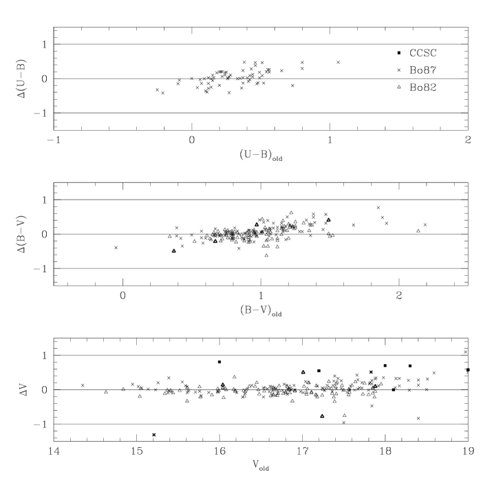
Figure 2: Comparison of new photometry to previous photographic results. CCSC: Crampton et al. (1985); Bo87: Battistini et al. (1987); Bo82: Buonanno et al. (1982). Bold symbols are objects for which another photometric method agrees better with our results.

We compared our optical photometry to published photometry, separating the previous work by method (photoelectric, photographic, or CCD). Figures 1, 2, and 3 and Table 3 show the comparisons, in the sense (previous photometry$-$this work), for the various colors and filters. As expected, the scatter increases with $V$ magnitude, but there is no evidence of a zeropoint offset or a varying slope, with the exception noted below. In many objects where there is a large discrepancy between one type of published photometry and our new work, our work agrees much better with one of the other types of published photometry. These points are marked with bold symbols in the figures. These large disagreements between the various photometry sources are disappointing but unsurprising; the last line of Table 3 shows that, while the photographic and photometric zeropoints agree well, there is a large RMS scatter between the data sets. Overall, we find that the published photometry is consistent with our new data.

There was one published data set with which our results show marked disagreement - the CCD photometry of bulge clusters from Battistini et al. (1993). Our B V colors are bluer and our V R colors redder than theirs, in each case by approximately 0.3^m. An obvious explanation, that our $V$ magnitudes were 0.3^m fainter, was not the case – our $V$ magnitudes agree well with theirs. The V R colors of Battistini et al. are bluer than those seen for most globulars in M31 or the Galaxy, so we suspect that there may be systematic problem in their photometry. Their B V colors are redder than those of the average Galactic globular, but this is not unreasonable since these clusters are near the M31 bulge and hence are more likely to be metal-rich (and intrinsically red). Other clusters in the same fields, although further from the galaxy nucleus, show no large offsets against previous photometry, and a check of magnitudes on our “raw” and “galaxy subtracted” CCD frames shows that the galaxy subtraction procedure did not substantially change the B V colors.

There also appears to be a small offset in our $V\!-\!I$ colors: most of this is due to a few clusters with large offsets, and the median offset is consistent with zero. For the clusters where we disagree with Mochejska et al. (1998) they note that their $I$ magnitudes are suspect due to nearby bad pixels. We have no explanation for the other large offsets, except to note that our galaxy subtraction procedure did not cause large changes in the $V\!-\!I$ colors. There is little comparison data for our V R and $V\!-\!I$ colors, so we made a second inspection of the photometric solutions in these colors. Our standard stars covered a wide range in colors, and we found no bias in the residuals as a function of color, so we are confident that any systematic errors affecting the $R$ and $I$ photometry are small.

3.2 Near-infrared photometry

Most of our new near-infrared data on the M31 clusters was taken with the SAO IR camera (Tollestrup & Willner, 1998) on the 1.2m telescope at FLWO, on 1998 Oct 27 and 28; conditions on both nights were photometric. This two-channel camera has a 5′  field of view, which required that we observe objects individually rather than attempting to map the entire galaxy. We observed the objects without published IR photometry in order of their $V$ magnitude, and collected photometry for 122 new objects. We also obtained photometry of four objects from the 2MASS (Skrutskie et al., 1997) scans of M31; these scans covered most of the galaxy but the short integration time of 6 seconds meant that only the brightest objects had acceptable signal-to-noise.

Our near-IR observations of objects and standard stars consisted of 5 to 9 dithered frames in each of $J$ and $K$ per object. Total integration times ranged from 140 to 240 seconds. Data reduction for the IR data consisted of the following steps: application of a non-linearity correction, dark subtraction, flat-fielding, sky-subtraction, registration, and co-addition. We made use of P. Hall’s phiirs package and a number of our own IRAF scripts.

Flat fields were constructed by median-combining about 100 M31 cluster frames which did not include the galaxy nucleus. Two sky-subtraction methods were used: for standard stars and objects far from the nucleus we used running skies (usually a median of the 8 frames nearest in time), and for each object near the nucleus we observed a separate sky position, median-combined those images to make a sky frame, and subtracted the sky from the object frames. We performed galaxy subtraction on some of the co-added object frames, again using the ring median filter.

We observed about a dozen Elias et al. (1982) standard stars per night, and fit a two-component (zeropoint and airmass coefficient) photometric solution using their measured aperture magnitudes. We tried including a color term in the solution, but this did not improve the fit. Others’ experience also indicates that the color term for this camera is negligible, so we did not use it in our final solution. Residuals from the photometric solution were $\lesssim 0.02^{m}$ for both nights and both filters.

We identified the clusters and candidates on the final coadded fields by visual comparison with the optical finding charts. In addition to the target objects, many fields contained brighter objects with published photometry and/or additional, fainter objects. We measured aperture magnitudes for all the identified objects, again using apphot. We constructed growth curves for the brightest clusters and found that a 12-arcsec diameter aperture contained $\sim 95$% of the M31 clusters’ light. This is comparable to the aperture sizes used in most previous IR photometry; the fact that a smaller aperture is required for IR than for optical photometry is a consequence of the better seeing in the IR.

Following the procedure used for the optical photometry, we performed both “internal” (night-to-night and frame-to-frame) and “external” (previously published) photometry comparisons. The within-night scatter is the standard deviation of the differences in magnitudes of the same object on different co-added images, and it is approximately $0.06^{m}$ in $J$ and $0.08^{m}$ in $K$. In both $J$ and $K$ this scatter is $\sim 0.02^{m}$ larger than the average photometric errors, a measure of how “photometric” the conditions were. The scatter between observations of the same object on adjacent nights is comparable to the within-night scatter.

Figure 4 shows the results of the external photometry comparison. Because the camera’s field of view is small compared to the size of M31, and because we observed objects without previous photometry, the number of comparison objects is small. For the 24 objects with published photometry, both offsets are consistent with zero: $\overline{\Delta K}=-0.014\pm 0.031$, $\overline{\Delta J}=+0.001\pm 0.019$. The standard deviations of the photometry differences ($\sim 0.15^{m}$ in $K$ and $\sim 0.10^{m}$ in $J$) are larger than is comfortable, but the small numbers make it difficult to tell if this is due to some systematic problem in our own photometry or in the previous work.

3.3 Spectroscopy

We acquired new spectra of 61 cluster candidates, most with the Keck LRIS spectrograph (Oke et al., 1995) in 1995 December and 1996 September, and a few with the MMT Blue Channel spectrograph in 1993 October. With LRIS we used a 600 line/mm grating, giving 1.2 Å/pixel dispersion from 3670-6200 Å and a resolution of 4-5Å. With the Blue Channel, we used a 300 line/mm grating, giving 3.2 Å/pixel dispersion, spectral coverage from 3400-7200 Å, and 9-11 Å resolution. Typical exposure times were 4 minutes with LRIS and 15 minutes with the Blue Channel. We performed the usual reduction steps for CCD spectra (bias subtraction, flat fielding, sky subtraction) using IRAF. The wavelength calibration used arc lamp spectra taken in temporal proximity to the object spectra, and the relative flux calibration used standard star spectra taken on the same or adjacent nights; both were also done in IRAF.

We used visual inspection of the spectra and radial velocity information to determine which objects were bona fide globular clusters. Objects with strong Na D lines, narrow line widths, continuum slope more appropriate to stars, and/or low radial velocities were classified as stars, while objects with large radial velocities were classified as galaxies. Both classifications are noted in Table 5. We determined velocities of the clusters by cross-correlating their spectra against spectra of template clusters with well-determined velocities (225-280, 163-217, 158-213), taken on the same night, using the xcsao cross-correlation package. The new velocities are in Table 5. Figure 5 shows examples of some of the new Keck spectra.

Several of the clusters with new spectra had spectra with large Balmer absorption lines, but with cross-correlation velocities too large for them to be likely Galactic A stars. Examining the archived spectra used by HBK, we identified several more clusters with similar spectra, bringing the total number to 15. We tentatively classify these objects as young globular clusters; other authors, including Sargent et al. (1977) and Elson & Walterbos (1988), have similarly classified some of these objects. We flag these objects as ‘young?’ in Table 5 and do not attempt to determine their metallicities. A detailed examination of these objects will follow in a subsequent paper.

We modified the iraf task sbands to compute absorption line indices according to the prescription of Brodie & Huchra (1990). We tested this modified task on the archived MMT spectra of HBK and found excellent agreement: our measurements differed from the published values (Huchra, 1996) by less than 0.01^m, on average, for all indices. We measured the indices on flux-calibrated versions of our new spectra and determined the index errors using non-fluxed versions of the same spectra, again according to the prescription given in Brodie & Huchra (1990). The measured indices were combined using the metallicity calibration defined in that paper to determine metallicities; the resulting metallicity measurements are in Table 5. It is clearly possible to do a more detailed metallicity analysis using the new Keck spectra, since they have better signal-to-noise than most of the MMT spectra used by HBK; however, since most of the spectroscopic data still come from that paper, we used its methods to maintain consistency across the cluster sample.

3.4 Data summary

We have compiled the results of our new photometry and spectroscopy with the existing data from the literature into a final catalog of M31 cluster data. Optical photometry is the only subset of the data where our new data significantly overlaps with published work; to keep this data set as uniform as possible, we used our photometry in preference to published data unless our photometric errors were larger than $0.10^{m}$. Of 435 clusters and cluster candidates, 268 have optical photometry in four or more filters, 224 have near-infrared photometry, 200 have velocities, and 188 have spectroscopic metallicities. This catalog is the basis for the analysis to follow in the next section and is, to our knowledge, the most comprehensive catalog of information available for M31 globular clusters and plausible cluster candidates. The catalog is available electronically at http://cfa-www.harvard.edu/~huchra/m31globs/. The electronic version contains additional information not given in this work, e.g. duplicate object names.

4 Analysis

Our classification of some M31 clusters as possibly young from their spectra made us suspect that the cluster catalog could be contaminated by other young objects. We checked this using B V as a rough age indicator, since this color is available for the largest number of objects. We found that most of the ‘young’ clusters were blue, with an average B V  of $0.37\pm 0.07$; the average B V for all objects in the catalog was $0.87\pm 0.02$. The two bluest Galactic globulars in the June 1999 version of the Harris (1996) catalog have $(B\!-\!V)_{0}=0.40$ and 0.42, but these are the most- and least-reddened clusters in the catalog (Terzan 5 has $E_{B-V}=2.37$ and NGC 7492 has $E_{B-V}=0.0$), so their colors are somewhat suspect. The next bluest clusters have $(B\!-\!V)_{0}=0.55$. It seems likely, then, that objects in M31 with $B\!-\!V<0.55$ are not true globular clusters. There are 49 such objects in our catalog, and their other colors are blue as well: for example, they lie along an extension of the sequence in B V vs. U B formed by the redder objects. We removed these blue objects and the remaining ‘young’ clusters (which might be reddened and thus have $B\!-\!V>0.55$) from our dataset before beginning the analysis. B V color is not a perfect selection criterion, of course: some objects do not have B V values, and some may have photometric errors which put them on the wrong side of the boundary. However, except for a few clusters with poor-quality spectra, all of the spectroscopically-observed clusters with $B\!-\!V<0.55$ had already been identified as young from their spectra. This suggests that our B V criterion is reasonable.

4.1 Reddening

Previous photometric studies of the M31 GCS have dealt with the problem of determining the cluster reddening in several ways. Frogel et al. (1980) (hereafter FPC) corrected the colors of 35 clusters for reddening, using the reddening-free parameter $Q_{K}$ from unpublished spectroscopic work by Searle. Crampton et al. (1985) used the intrinsic colors of the same 35 clusters to calibrate $(B\!-\!V)_{0}$ as a function of their spectroscopic slope parameter $S$. Numerous authors (e.g. Iye & Richter, 1985; Bajaja & Gergeley, 1977; Sharov, 1977) have used the globular clusters as reddening probes, often by assuming them to have a single intrinsic color. Most studies of the M31 GCLF (Reed et al., 1992, 1994; Secker, 1992; Kavelaars & Hanes, 1997; Gnedin, 1997) studied only clusters outside the ellipse used by Racine (1991) to define the outer boundary of the M31 disk. These authors assumed that only foreground Galactic extinction affected these ‘halo’ clusters.

For the disk clusters, there is almost certainly extinction due to dust in the disk of M31, so merely correcting for Galactic extinction is not sufficient. Determining the reddening from the total HI column density and dust-to-gas ratio is also not sufficient, since the clusters lie at different (and unknown) distances along the line of sight through the M31 disk. The assumption that the halo clusters suffer only foreground reddening may also be incorrect: recent far-infrared observations of spiral galaxies (Nelson et al., 1998; Alton et al., 1998) indicate that the dust is more extended than the starlight. It is important to test this by determining the reddening of the halo clusters.

With our larger database of multicolor photometry we attempted to determine the reddening for each individual cluster, using correlations between optical and infrared colors and metallicity, and by defining various ‘reddening-free’ parameters. To calibrate these methods we used the June 1999 version of the Harris (1996) database of Galactic GC parameters. This database contains colors from Peterson (1993) and Reed (1996), reddening values from multiple sources (mainly Reed et al. 1988,Webbink 1985, and Zinn 1985), and metallicities from multiple sources (mainly Zinn 1985 and Armandroff & Zinn 1988). We corrected the colors for reddening using the $R_{V}=3.1$ extinction curve of Cardelli et al. (1989). There are two major unavoidable assumptions in this procedure: that the extinction law and the globular cluster intrinsic colors are the same in the Galaxy and in M31. There is conflicting evidence on whether this first assumption is correct: Massey et al. (1995) find $E_{U-B}/E_{B-V}=0.4-0.5$, Iye & Richter (1985) found this ratio to be $1.01\pm 0.11$, and Walterbos & Kennicutt (1988) found it to be $0.6\pm 0.2$. Since there is no alternative optical-infrared extinction curve for M31, using the Galactic curve is the only option. We will show below that this is reasonable.

We performed linear regressions of intrinsic optical colors against metallicity for the 88 Galactic clusters with $E_{B-V}<0.5$. Colors used were $(B-V)_{0},(B-R)_{0},(B-I)_{0},(U-B)_{0},(U-V)_{0},(U-R)_{0},(V-R)_{0},(V-I)_{0},(J-K)_{0}$, and $(V-K)_{0}$. The correlation coefficients $r$ ranged from 0.91 for $(U-R)_{0}$ to 0.77 for $(V-R)_{0}$; $(V-R)_{0}$ is a poor metallicity indicator because of its small range and we do not consider it further. The color excess is determined from the observed color, the metallicity-derived intrinsic color, and the reddening ratio from Cardelli et al. (1989):

$$(X-Y)_{0}=a{\rm[Fe/H]}+b$$ (1)

$$E_{B-V}=\frac{E_{B-V}}{E_{X-Y}}[(X-Y)-(X-Y)_{0}]$$ (2)

We use $X-Y$ as generic notation to represent any color.

These color-metallicity relations allow us to check the assumption that the reddening laws in M31 and the Galaxy are the same. To do this, we used the colors of the ‘old’ M31 clusters with spectroscopic metallicities. For each cluster, we used the above linear regressions to determine the color excess in each color, then derived the various reddening ratios by dividing these color excesses by the color excess for B V, also determined from the intrinsic color-metallicity relation. Within the (admittedly large) uncertainties, the medians of these reddening ratios over all clusters were consistent with the Galactic values; see Table 6. This result validates our use of the Galactic extinction curve to determine the reddening. We must still show that the color-metallicity relations are the same for the two sets of clusters and we do so in the following section.

To estimate the reddening for objects without spectroscopic data, we also determined relationships between ‘reddening-free parameters’ and intrinsic colors. We derived all six possible reddening-free parameters (hereafter referred to as Q-parameters) from the same Galactic cluster $U\!BV\!RI$ data used to calibrate the color-metallicity relations. The Q-parameters are defined as:

$$Q_{XYZ}\equiv(X-Y)-\frac{E_{X-Y}}{E_{Y-Z}}(Y-Z)=(X-Y)_{0}-\frac{E_{X-Y}}{E_{Y-Z}}(Y-Z)_{0}$$ (3)

We then regressed these against the clusters’ intrinsic colors, and used the results to determine the color excess. Schematically:

$$Q_{XYZ}\Rightarrow(X-Y)_{0}\Rightarrow E_{B-V}$$ (4)

The correlation coefficients for the Q-parameters were poorer than those for the color-metallicity relations, ranging from 0.80 for $Q_{BVR}$ to 0.27 for $Q_{VRI}$. Since there is significant scatter in all of these correlations (due to age or ‘second parameter’ effects?) applying them will yield only a rough estimate of the individual cluster reddening, and we do not attempt to treat the results in a statistically rigorous manner.

Our final reddening determination used seven of the nine colors in Table 6 (we dropped U B and $J\!-\!K$, since these colors are not very sensitive to reddening) and all six Q-parameters. For each of the two methods we averaged the results over all colors or parameters to produce one value of $E_{B-V}$ per method. The standard deviations of these averages serve as an estimate of the precision of the methods. We tested the methods first on 25 heavily-reddened Galactic clusters not used for the calibration. The results were encouraging – the precision of both methods, defined as $\sigma_{E_{B-V}}/\overline{E_{B-V}}$, had a median value of $\sim 7$%. The two methods agreed quite well both with each other and with the color excesses from the Harris catalog: the average offset between $E_{B-V}$ from the Q-parameter method and the Harris value was $0.03\pm 0.03$; for the color-metallicity method the average offset was $0.00\pm 0.02$ (see Figure 6).

To determine the reddening for the M31 clusters we combined the results from the two methods, subtracting 0.03 from the Q-method results because of the offset noted in the previous paragraph. We examined the errors in the cluster reddenings from the two methods, and determined that the errors were the same when the error in [Fe/H] was approximately 0.4, and that the error in the metallicity-derived $E_{B-V}$ increased dramatically for ${\sigma}_{\rm[Fe/H]}>0.7$.

The $E_{B-V}$ and [Fe/H] errors are related by

$${\sigma}_{E(B-V)}=\left|\frac{\partial\overline{E_{B-V}}}{\partial{\rm[Fe/H]}}\right|{\sigma}_{\rm[Fe/H]}=\left(\frac{1}{N}\sum\frac{E_{B-V}}{E_{X-Y}}a_{X-Y}\right){\sigma}_{\rm[Fe/H]}$$ (5)

(where $N$ is the number of colors and $a$ is the same as in equation 2). We weighted the metallicity-derived $E_{B-V}$ by the inverse of the bracketed term in the above equation. The zeropoint of the weighting was set so that the weight of $E_{B-V}({\rm[Fe/H]})$ would be zero at ${\sigma}_{\rm[Fe/H]}=0.7$, and the weight for $E_{B-V}({\rm Q})$ was set to give the two methods equal weight at ${\sigma}_{\rm[Fe/H]}=0.4$.

To check our results, we compared our reddenings with the $E_{V-K}$ given for 34 clusters in FPC. A typical error in our values of $E_{B-V}$ for these clusters was 0.04. For 24 of these clusters FPC quote $E_{V-K}=0.28$, which corresponds to $E_{B-V}=0.10$, their value for the foreground reddening. For these clusters our $E_{B-V}$ ranges from 0.01 to 0.18 with a mean $E_{B-V}=0.13\pm 0.02$. For the 10 clusters with larger reddening, we find the median $E_{B-V}/E_{V-K}=2.7\pm 0.2$, which is consistent with the Cardelli et al. value of 2.75, or the FPC value of 2.8.

We also compared our results with the predicted $E_{B-V}$ from the Galactic dust maps of Schlegel et al. (1998), hereafter SFD. Since their map does not account for reddening internal to the M31 disk, we compared only reddening for objects in the halo, as defined by Racine (1991). We were able to determine a reddening for 60 of these clusters, with typical errors of 0.06 in $E_{B-V}$. The mean offset (SFD$-$our value) is $-0.02\pm 0.01$, consistent with zero. However, the standard deviation of the offset (0.08) is large, and, for low reddening, our values scatter between 0 and 0.2 and show little correlation with the SFD results (which have values between 0.05 and 0.1). The SFD maps show a large reddening for one cluster (462-000), and for it the agreement is fairly good: the SFD maps give $E_{B-V}=0.29$ and we find $E_{B-V}=0.28\pm 0.16$. From the comparisons with SFD and FPC, we estimate that our values of $E_{B-V}$ have total errors between 0.05 and 0.10. These are large errors, but we believe this method is preferable to the alternatives of correcting only for the foreground reddening or doing no reddening correction at all.

We estimated reddenings for all the M31 clusters with sufficient data, a total of 314 objects. Some values are more reliable than others: unreliable measurements are those with with no reddening errors (those with only one color-metallicity relation or Q-parameter) and those with large reddening errors (arbitrarily chosen as $\sigma_{E_{B-V}}/\overline{E_{B-V}}>0.5$ for $\overline{E_{B-V}}>0.15$, $\sigma_{E_{B-V}}/\overline{E_{B-V}}>1.0$ for $\overline{E_{B-V}}<0.15$). We do not use these reddenings in the analysis that follows. The distribution of the 221 reliable reddenings (Figure 7) has a mean of $E_{B-V}=0.22$, a median of $E_{B-V}=0.16$, and a standard deviation of 0.19. Three-quarters of the clusters have $E_{B-V}<0.27$. The largest ‘reliable’ reddening is that of 037-B327, $E_{B-V}=1.38$; van den Bergh (1969) notes that this cluster is “the most highly-reddened cluster known in M31”. If this reddening value is correct, 037-B327 is twice as luminous as 000-001 ($=$G1), one of the brightest M31 GCs. Assuming an M31 distance modulus of 24.47 (Stanek & Garnavich, 1998; Holland, 1998) means that 037-B327 has $M_{V}\approx-12$ and is more than four times as luminous as the brightest Galactic GC ($\omega$ Cen at $M_{V}=-10.29$; Harris, 1996). This object is puzzling: as van den Bergh states, there is no obvious reason why the intrinsically brightest GC in M31 should also be the most heavily-reddened. However, the nature of 037-B327 is still uncertain: the reddening estimate is from color information alone, and a spectrum of this object would be extremely valuable.

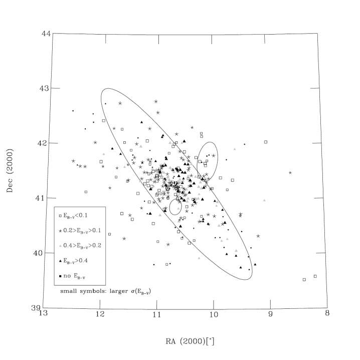
Figure 8: Map of M31 globular clusters in RA and Dec, in groups according to reddening. Large ellipse is M31 disk/halo boundary as defined by Racine (1991); smaller ellipses are $D_{25}$ isophotes of NGC 205 (NW) and M32 (SE).

All of the reddening values are shown in as functions of position in Figure 8. The maps appear reasonable in that the objects with the lowest reddening are spread across the disk and halo, while those with the highest reddening are concentrated in the galaxy disk. The higher-reddening clusters in the disk tend to lie on the northwest side of the major axis. This accords with statements in previous work (Iye & Richter, 1985; Elson & Walterbos, 1988) that this side of the disk is nearer to us along the line of sight. We note that a substantial number of clusters outside the ‘halo’ boundary have $E_{B-V}>0.1$. While some of these values are undoubtedly due to the large errors in our method, some clusters (such as 004-050, with $E_{B-V}=0.19\pm 0.04$) have reddening values that are very consistent over a number of colors and Q-parameters. It seems unlikely that some systematic problem in our method or photometry could affect all of the individual colors to make them give the same erroneous reddening. Two possibilities remain: (1) the M31 dust distribution extends to greater projected distances than previously suspected, and/or (2) the Galactic foreground extinction in the direction of M31 is patchy on scales smaller than the SFD spatial resolution of 6.1′. In either case, the assumption that the M31 halo clusters are subject to only foreground reddening is in some doubt and should be re-examined.

4.2 Color-metallicity relation

We showed in Section 4.1 that the assumption of a similar reddening law in M31 and the Galaxy was reasonable. The second major assumption made in our reddening correction procedure was that the relation between intrinsic color and metallicity is the same for M31 GCs and Galactic GCs. We tested this assumption by doing BCES bisector linear fits (as described in Akritas & Bershady, 1996) of color against metallicity for the M31 and Galactic clusters and comparing the results. The bisector fit is appropriate since we are interested in both the case where metallicity is used to predict color, as in the determination of reddening, and the case where color is used to predict metallicity, as follows in Section 4.4. (To do the actual predictions we used the BCES(Y$|$X) fit, an extension of the ordinary least-squares fit which allows for measurement error in both variables and intrinsic scatter. For reference, these fits for the Galactic data are given in Table 7.)

For the Galactic color-metallicity fits we used the same data used to determine the color-metallicity relations in Section 4.1; we estimated the intrinsic color errors as:

$${\sigma}_{X-Y}=({{\sigma}_{\rm phot}}^{2}+({\sigma}_{E(B-V)}E_{X-Y}/E_{B-V})^{2})^{1/2}$$ (6)

We set ${{\sigma}_{\rm phot}}$ to $0.02^{m}$, as this is a typical uncertainty in Reed (1996), one of the main sources of integrated colors, and ${\sigma}_{E(B-V)}$ as $0.1E_{B-V}$, following Harris (1996). We set $\sigma_{\rm[Fe/H]}$ for the Galactic clusters to 0.10 dex; typical uncertainties in Zinn (1985) (one of the major sources for Harris, 1996) are 0.15 dex, but many of the [Fe/H] values are averages from several sources. For the M31 fits we used 101 M31 clusters with reliable reddening and $\sigma_{\rm[Fe/H]}<0.5$ dex. We estimated color errors using equation 6, with ${{\sigma}_{\rm phot}}$ set to $0.04^{m}$ and ${\sigma}_{E(B-V)}$ to our measured value.

The BCES method produces estimates of the uncertainty in the slopes and intercepts of the linear fits, so one way to compare the two sets of fits is to compare the ratio of the parameter differences to the parameter uncertainty. However, unlike the case for ordinary least-squares fitting, the distribution of this ratio in the case of the null hypothesis is unknown, so it is impossible to determine its statistical significance. A more empirical approach is to simply compare the predictions of the two fits. We determined the differences in color predicted by the two fits at the metal-rich (red) and metal-poor (blue) ends of the data range, and compared these to the rms color residuals of the fits. We found the differences between the Galactic and M31 fits to be comparable to the fit residuals for all the colors.

The $(V\!-\!K)_{0}$ and $(J\!-\!K)_{0}$ fits are shown in Figure 9; these deserve particular attention for several reasons. The Galactic relations as originally derived by Brodie & Huchra (1990) rely on only 23 low-reddening calibrators in their Table 5A. Only four of these Galactic calibrators have ${\rm[Fe/H]}>-1.2$. To maintain consistency with the optical color-metallicity fits, we did the optical-infrared color-metallicity fits using the metallicity and reddening values in Harris (1996), rather than those in Brodie & Huchra’s table. We also added the 14 “high-reddening” clusters in their Table 5B to see whether this made a difference to the fits. As Figure 9 shows, adding the additional clusters made a difference for $(V\!-\!K)_{0}$, bringing the fit closer to that for the M31 clusters (the second $(V\!-\!K)_{0}$ row in Table 7 shows the Galactic fit with all clusters included). Calibrating the color-metallicity relation with a small number of clusters means that even a small change in the input data can change the result.

For $(V\!-\!K)_{0}$ there are several M31 clusters which are either too blue for their metallicities or too metal-rich for their colors, compared to the Galactic clusters and the bulk of the M31 clusters. We have examined the spectra of these clusters and their photometry, and find no obvious problems with either. These clusters are not different from the bulk of M31 clusters in any obvious way (location, reddening, H$\beta$ strength, etc.), and we are unable to explain their anomalous colors.

There is little difference in the $(J\!-\!K)_{0}$ fit when all clusters, instead of just low-reddening ones, are included. This is unsurprising since $J\!-\!K$ is much less sensitive to reddening than $V\!-\!K$. However, the $(J\!-\!K)_{0}$ vs. metallicity fit shows much larger rms residuals for the M31 clusters than the Galactic clusters. If we restrict the M31 data to the 31 clusters brighter than $V=15.5$ – presumably these should have smaller photometric and spectroscopic errors because they are brighter – the residuals are much closer to the Galactic values, although the fit does not change significantly. This suggests that errors in the $J\!-\!K$ photometry may have been underestimated, and points to the need for precise $J\!-\!K$ colors if $(J\!-\!K)_{0}$ is to be used as a metallicity indicator. As Table 7 shows, $(J\!-\!K)_{0}$ is not as sensitive to metallicity as most of the other colors; its advantage as a metallicity indicator is its insensitivity to reddening.

Eighty-seven of the cluster candidates in our sample of 221 with ‘reliable’ reddening (as defined in the previous section) have no spectroscopic information, so we attempted to estimate their metallicities from their intrinsic colors. We applied the BCES(Y$|$X) fits of metallicity as a function of color, and averaged the resulting metallicities over all available colors. As in the reddening determination, the standard deviation of the metallicities from individual colors was used as the error estimate. We tested this procedure by using it on the clusters with spectroscopic information; this includes all the clusters used to do the metallicity-color fits as well as additional objects with large metallicity errors. The results are shown in Figure 10; the mean offset (spectroscopic$-$color-derived metallicity) is $0.020\pm 0.021$, there is no evidence of a bias in the prediction with metallicity, and the largest offsets are for objects with large errors in color- or spectroscopically-determined metallicity or both.

Applying the method to the clusters without spectroscopic data produced equally encouraging results. 57% of the color-derived metallicities had uncertainties ${\sigma}_{\rm[Fe/H]}<0.5$, compared to 76% within the same error range for spectroscopic metallicities. Six objects had very large or small values of [Fe/H] ($>+0.5$ or $<-2.5$); these had only a few colors and large errors in their derived [Fe/H]. These objects do not lie on the same two-color sequences as the confirmed globular clusters, so we suspect that they are either compact background galaxies, compact H II regions, or foreground stars. We do not include these outlying metallicities in the analysis that follows.

4.3 Color distributions

We analyzed the distribution of intrinsic colors for the 221 M31 GCs with reliable reddening. The histograms of colors are shown in Figures 11-13, and parameters of the color distributions are given in Table 8. For comparison, the table also shows the mean intrinsic colors of the Galactic clusters (optical from Harris (1996), $(V\!-\!K)_{0}$ and $(J-K)_{0}$ from Brodie & Huchra 1990). The mean colors of the M31 clusters are consistent with corresponding Galactic mean colors. The large standard deviations in the M31 cluster colors incorporating $U$ probably reflect the larger photometric errors in this filter. $(V\!-\!K)_{0}$ is notable for having a larger range ($\sim 1.5^{m}$) than most other colors. This is, of course, the basis for its use as a metallicity indicator. $(V\!-\!R)_{0}$ is notable for having a very small range; as Reed et al. (1992) reported, this can be exploited to discriminate against background galaxies (which have $(V\!-\!R)_{0}\gtrsim 0.7$) in cluster searches.

We tested the color distributions of the M31 clusters for bimodality using the KMM algorithm (McLachlan & Basford, 1988; Ashman et al., 1994). The input to this algorithm includes the individual data points, the number of Gaussian groups to be fit, and a starting point for the groups’ means and dispersions (the final solution is not very sensitive to the starting points unless there are many outliers). We used the results of Ashman & Bird (1993) to choose our starting points: they found two groups of M31 clusters with ${\rm[Fe/H]}=-1.5$ and $-0.6$, with the metal-poor clusters comprising two-thirds of the total. Our input data specified two groups, with the bluer group twice as large, and the two mean colors corresponding to ${\rm[Fe/H]}=-1.5,-0.6$ from our color-metallicity relations (Section 4.2). The predicted mean colors for the two groups appear in the last two columns of Table 8. We specified the same dispersions for both groups in each color; in this case (‘homoscedastic’ fitting as opposed to ‘heteroscedastic’) the $p$-value returned by KMM adequately measures the statistical significance of the improvement in the fit in going from one to two groups. As a rough estimate, we specified a value of 80% of the overall dispersion in Table 8 as the starting point for the groups’ dispersions in each color.

The hypothesis of a unimodal color distribution was rejected for only three colors: $(U\!-\!V)_{0}$ and $(U\!-\!R)_{0}$ at the $95$% confidence level and $(V\!-\!K)_{0}$ at the $92$% level. The mean colors of the two groups in all three colors correspond to metallicities of approximately $-1.5$ and $-0.6$. These three colors are the most sensitive to metallicity (Table 7), so it would be expected that they would show the strongest evidence for bimodality. In the other colors, the photometric errors are probably large enough to mask any color separations between the metal-rich and metal-poor populations. Visual inspection of the color histograms suggested that these same three colors might actually have trimodal distributions. We tested for this, again using KMM, and found that three-group fits were not superior to either one- or two-group fits for $(U\!-\!V)_{0}$ and $(U\!-\!R)_{0}$. Three groups were preferred to one or two for $(V\!-\!K)_{0}$. We are reluctant to claim a physical meaning for this, since this color is the most sensitive to both photometric errors (separate optical and infrared photometry is combined) and reddening. In the following section we show that two metallicity groups are preferred.

Figure 14 shows the distribution of $(V\!-\!I)_{0}$, which is often used as a metallicity indicator for globular cluster systems despite its fairly low metallicity sensitivity (see Table 7). From HST imaging in $V$ and $I$, Kundu (1999) finds that 25-50% of the GCSs of a sample of $\sim 50$ galaxies show evidence for bimodal color distributions; Gebhardt & Kissler-Patig (1999) find similar results. The bottom two panels of the figure show the color distributions for elliptical galaxy GCSs with and without bimodality. The M87 (data from Kundu et al., 1999) and NGC 5846 GCs (data from Forbes et al., 1997b) clearly show bimodal distributions in $(V\!-\!I)_{0}$. The ‘unimodal E’ panel is the sum of 12 elliptical GCS color distributions which Forbes et al. (1996) find not to be bimodal; although the histogram bins are larger in these data, the distribution is remarkably symmetric and unimodal. Comparing the color distribution for the ellipticals and spirals yields two interesting conclusions: first, M31 and the Galaxy clearly lack the extremely red (and presumably metal-rich) GCs found in massive ellipticals. Second, the blue peaks of the M87 and NGC 5846 color distributions are at approximately the same color as the M31 and Galactic peaks. This is consistent with the finding that these galaxies’ metal-poor GC populations and the total M31 GC population have approximately the same mean metallicity (${\rm[Fe/H]}\approx-1.2$; Forbes et al. (1997a) and the following section), and is also an interesting hint of a possible connection between ellipticals’ metal-poor GCs and spirals’ GCs.

The Galactic GCs (see, e.g. Côté, 1999) and the M31 GCs (Ashman & Bird, 1993, and the following section) are known to have bimodal metallicity distributions, and we have just shown that some M31 cluster colors are bimodal – why not $(V\!-\!I)_{0}$? We did Monte Carlo simulations of our observations of the $V\!-\!I$ distribution, and, as suggested above, we found that observational errors in the reddening and photometry can wash out the signature of bimodality. We predicted the M31 GCs’ ‘true’ $(V\!-\!I)_{0}$ colors from their spectroscopically-determined [Fe/H] (see the middle panel in Figure 14); we found this ‘true’ distribution to be bimodal at the $>99$% confidence level. We then added to each color datum a Gaussian random error, drawn from a distribution with mean of 0 and standard deviation expected from the errors in our photometry and reddening determination. Of the 1000 color distributions generated in this manner, KMM detected bimodality in only about 250, implying that observational errors wash out the bimodal signal three-quarters of the time. Detection of multiple populations in GCS color distributions thus clearly requires precise photometry and/or the use of metal-sensitive colors.

We examined the correlation of M31 cluster intrinsic colors with distance from the galaxy’s center, using the coordinate system of Baade & Arp (1964), as defined in HBK. In this system, $X$ is the projected distance from the center of M31 along the major axis (positive $X$ is to the northeast), $Y$ is the projected distance along the minor axis (positive $Y$ is to the northwest), and $R$ is the projected radial distance from the galaxy center, $R=\sqrt{X^{2}+Y^{2}}$. Ideally we would use the true spatial distance and not the projected distance from M31, but this information is not available for the M31 GCs. We binned the clusters in 20′ bins in $X$ and $Y$ and 10′ bins in $R$, then calculated the weighted least-squares fit of the bin median colors against distance. It is well-known (Iye & Richter, 1985; Elson & Walterbos, 1988) that the observed colors of M31 clusters are redder for $Y>0$, because the northwest side of the M31 disk is closer to us and more clusters are projected behind it. If our reddening correction was adequate this trend should be removed from the intrinsic colors. None of the colors showed a significant trend with $X$ or $Y$, confirming that our reddening correction worked. More surprising was the fact that none of the colors showed a significant trend with $R$; such a trend would be expected if there was any gradient in the metallicity of the system. However, even a large metallicity gradient (for example, 0.5 dex over 100′) would produce a fairly small change in most colors ($\lesssim 0.15^{m}$) so perhaps photometric errors and scatter within the bins mask any true gradient.

Comparing the clusters’ location in two-color diagrams to models produced by population synthesis provides useful checks on our photometry and on the models’ accuracy. We obtained predicted colors for populations of ages 8 and 16 Gyr from three sets of models: Worthey (1996), Bruzual & Charlot (1996) (hereafter BC), and Kurth et al. (1999) (hereafter KFF). We used Worthey’s ‘vanilla’ models and his interpolation program to generate colors for values of [Fe/H] from $-2.0$ to $-0.1$ in steps of 0.1 dex. We used the Salpeter IMF versions of the Bruzual & Charlot and Kurth et al. models, without interpolation, and obtained colors at metallicities of $-2.33$ (KFF models only), $-1.63$, $-0.63$, $-0.32$, 0.07 and 0.47 dex. Worthey (1994) states that, compared to Galactic GCs, his models are too red by 0.08^m in B V and too blue by 0.03^m in $J\!-\!K$, so we corrected the model colors by these amounts. Worthey attributes these offsets to defects in the stellar flux library; since all three sets of the models share the same stellar atmosphere models we applied the same corrections to the BC and KFF models.

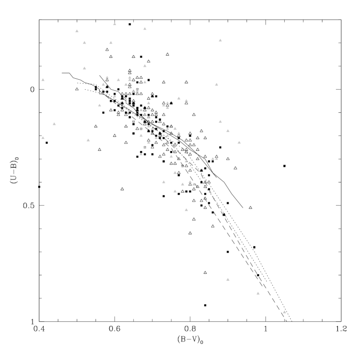
Figure 15: $(B-V)_{0}$ vs. $(U-B)_{0}$ for Galactic GCs (squares), confirmed M31 GCs (open triangles), and M31 GC candidates (shaded triangles). Lines are population synthesis models of ages 8 Gyr (bluer colors) and 16 Gyr (redder colors): Worthey (1996) (solid), Bruzual & Charlot (1996) (dashed), Kurth et al. (1999) (dotted). Models have been corrected as described in the text.

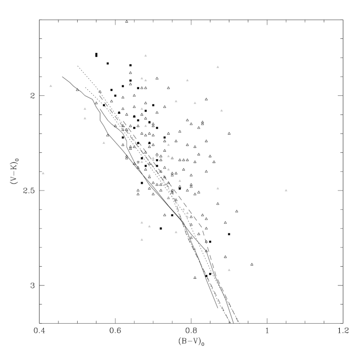
Figure 16: $(B-V)_{0}$ vs. $(V-K)_{0}$ for M31 and Galactic GCs. Symbols as in Figure 15.

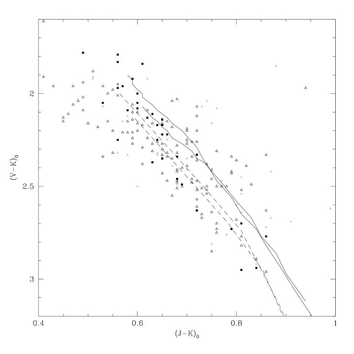
Figure 17: $(J-K)_{0}$ vs. $(V-K)_{0}$ for M31 and Galactic GCs. Symbols as in Figure 15; the KFF models do not predict $J$ so are absent from this figure.

In Figures 15-17 we plot two-color diagrams for M31 clusters, Galactic clusters and the models, using optical and IR colors often found in the literature. Confirmation that our photometry suffers no major systematic errors is provided by the fact that the Galactic and M31 clusters lie on essentially the same loci in all the diagrams. As expected, the M31 clusters show much more scatter than the Galactic GCs (because the photometric and reddening errors are larger), but much of this scatter is due to objects that are not confirmed clusters. It is clear from the diagrams that integrated photometry and model predictions are not precise enough to distinguish any possible age differences between the two sets of old clusters.

In Figure 15 the corrected models agree reasonably well with the data in B V and U B, although the agreement becomes poorer in the high-metallicity region. The models also agree fairly well with each other in these colors, which is not the case in Figures 16 and 17. The model disagreement is not surprising; Charlot et al. (1996) found a difference of $0.3^{m}$ in predicted $V\!-\!K$ between the solar-metallicity models of Worthey and those of Bruzual & Charlot. These authors attribute most of the discrepancy to differences in the underlying stellar evolution prescriptions. Shifting the Worthey models by $\sim 0.2^{m}$ to bluer $V\!-\!K$ to match the data in Figure 16 (since Figure 15 implies that the B V color is acceptable) would then require shifting the same models to bluer $J\!-\!K$ by $\sim 0.1^{m}$ to match the data in Figure 17. The shifts required for the BC and KFF models to fit the data in the B V/$V\!-\!K$ and $J\!-\!K$/$V\!-\!K$ planes are in the same direction, but about half the magnitude, as those required for the Worthey models. This arbitrary shifting of predicted colors to match the data does not uniquely determine the reasons for the disagreements between models and data. We speculate that the mismatches may be caused by problems in the treatment of the late stages of stellar evolution in the models, since most of the $K$-band light comes from evolved stars. The theoretical and observation photometric systems could also have systematic offsets. Clearly this is an area requiring more detailed examination by modelers, and the colors of globular clusters provide important constraints on the models.

In Figure 18 we plot [Fe/H] as a function of $(V\!-\!K)_{0}$. Some M31 GCs are too blue for their metallicities or too metal-rich for their colors, as discussed in Section 4.2. Covino et al. (1994) noted that some low-metallicity Galactic clusters were “exceedingly blue” with respect to the models of Buzzoni (1989); they attribute this to a systematic problem with the photometry. However, we find that the M31 clusters and Galactic clusters overlap in the region $(V\!-\!K)_{0}\lesssim 2.1$ (Figure 18), and that the $(V\!-\!K)_{0}$-[Fe/H] relations for the two sets of clusters are very similar at the metal-poor end (Figure 9). This implies that the Buzzoni (1989) models are too red, rather than the clusters being too blue, and indeed the Buzzoni models are about $0.1^{m}$ redder than the models we examine here. We showed in the previous paragraph that substantial shifts in model $V\!-\!K$ colors were required to match the clusters in two-color diagrams. Shifting the model $V\!-\!K$ to the blue to match the B V colors would make the model $V\!-\!K$ too blue for the clusters’ metallicities. This again emphasizes the difficulties of trying to match population synthesis models to cluster colors by applying uniform shifts for all metallicities.

4.4 Metallicity distributions

The metallicity distribution of a galaxy’s GCS can provide important clues to galaxy formation. For example, Zinn (1993) finds a significant metallicity gradient in the Galactic ‘old halo’ clusters and no gradient in the ‘younger halo’. He interprets this and other properties of the Galactic GCS as evidence that the old clusters were formed in a monolithic collapse and the younger ones were accreted from satellite galaxies. Accordingly, we want to examine the distribution of cluster metallicities in M31, and to do so for the largest number of clusters. We thus include metallicities estimated from colors in our analysis, even though this method is not as precise as determining metallicity spectroscopically. We also include clusters for which we were unable to determine a reliable reddening value (usually because of inadequate photometric data) in the metallicity analysis.

To assess whether the determination of metallicities from colors has an effect on our results, we consider four data sets in our analysis of the metallicity distribution. Set 1 contains all the objects for which metallicities have been determined, regardless of method or error. Set 1a is a subset of this, containing only objects with ${\sigma}_{\rm[Fe/H]}<0.5$. Set 2 contains only objects with spectroscopic metallicities, and set 2a is the subset of these objects with ${\sigma}_{\rm[Fe/H]}<0.5$. The first step is to characterize the distribution of [Fe/H]. Table 9 shows that restricting the metallicities to spectroscopic alone slightly increases the mean metallicity, but not by a significant amount. This is good evidence that our color-derived metallicities are not systematically offset from the spectroscopic ones. A KS-test shows that the Galactic and M31 GC metallicity distributions are not drawn from the same distribution, unsurprising given the difference in mean metallicity; however, the shapes of the distributions are fairly similar (see Figure 19).

The asymmetric nature of the [Fe/H] distributions suggests the possibility of bimodality. We used the KMM algorithm to search for bimodality in the distributions, following Ashman and Bird as in Section 4.3. All four datasets showed bimodality, although including the color-derived metallicities made the detections only marginally significant. (see the $p$-values in Table 9). The [Fe/H] histograms and the Gaussian subgroups found by KMM are shown in Figure 19. Most clusters were assigned to the same (metal-rich or metal-poor) group regardless of which dataset was considered; however, there were about 20 clusters which showed substantial probability of membership in both groups and these switched groups from metal-rich to metal-poor depending on whether or not the large-error metallicities were included. This is the primary cause of the differences between samples 1/1a and 2/2a in Table 9. We conclude that these clusters cannot be unambiguously assigned on the basis of their metallicities alone, so we classify them as ‘intermediate’ and assign them to neither group. As with the color distributions, visual inspection of the metallicity histograms suggested the possibility of trimodality in the distribution. The results of running KMM with three groups specified were similar to those for the color distributions: three-group fits were worse than both one- and two-group fits. The mean colors of the metal-rich and metal-poor groups are generally within $0.05^{m}$ of the predicted colors in Table 8. This is not surprising since the metallicities used to predict these colors are close to the mean metallicities of the two groups KMM found. Perhaps more surprising is our failure to detect bimodality in most colors. This underscores the need for precise photometry if a single color is used to determine metallicity: such precision was obviously not achieved in our heterogeneous data set.

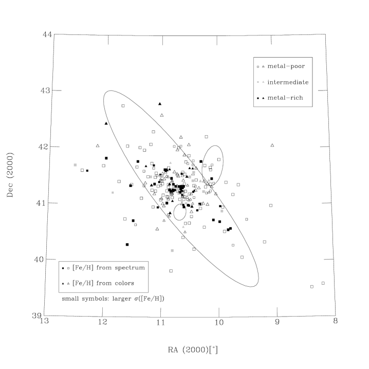
Figure 20: Projected location of metal-poor and metal-rich M31 clusters. Ellipses same as Figure 8.

Do these metal-rich and metal-poor groups represent the M31 equivalent of the Galactic disk (or bulge – see Côté 1999) and halo clusters? One way to find out is to see where the two groups lie in relation to the galaxy; we show the KMM assignments function of position on the sky in Figure 20. There are more metal-poor clusters at large projected radius, and as a result the median radius of the metal-poor clusters is about 50% larger than that of the metal-rich clusters. However, we find, as did HBK, that this is partly a selection effect: faint clusters are more easily discovered away from the disk, and these distant clusters are more likely to be metal-poor. When the sample is magnitude-limited at $V=16.5$ or $V=17$ we find that the median radius of the metal-poor clusters is about 30% larger than that of the metal-rich clusters, which is similar to the results of HBK. While most of the metal-rich clusters are projected onto the M31 disk, a few lie in the halo. Two of these clusters have color-magnitude diagrams (379-312 from Holland et al. (1997) and 006-058 from Fusi Pecci et al. 1996) that give values of [Fe/H] consistent with our spectroscopic values. The CMD of 384-319 (Couture et al., 1995) is so sparse that it cannot put any useful constraints on [Fe/H]. The existence of several metal-rich globular clusters in the Galactic halo (Terzan 7, NGC 6366, Pal 12; Da Costa & Armandroff 1995) also suggests that similar results for the M31 clusters are not unreasonable.

The kinematics of the metal-rich and metal-poor groups will be the most powerful determinant of their similarity (or lack thereof) to the two Galactic groups. We did not perform a detailed kinematical analysis, since two forthcoming velocity studies of the M31 clusters (Seitzer et al., 1999; Perrett et al., 1999) have substantially improved precision from HBK’s observations (the source of over three-quarters of our velocity data). We did repeat the HBK analysis (see their Figure 6 and Table 3), including our new velocities and using our division of the clusters, and found essentially the same results. At small projected distances, the metal-rich clusters rotate faster than the metal-poor clusters, and at large distances, there is essentially no difference between the two groups in either rotation velocity or velocity dispersion. The rotation velocity for all clusters at $X>10$′ is $59\pm 12$ km s^-1. The similarity in the kinematics of the metal-rich and metal-poor clusters hints that, unlike the Galactic clusters, the two groups of M31 clusters might be similar in age. Velocity errors and projection effects could confuse the situation, however, and more precise velocities and metallicities are needed.

How does the distribution of M31 GCS metallicity compare to that seen in other galaxies? Table M31 Globular Clusters: Colors and Metallicities compares some properties of spiral galaxies’ globular cluster systems. Spirals with detected GCSs which do not appear in this table (see Appendix of Ashman & Zepf (1998) and also Harris 1991) have generally been observed in only one filter, so no metallicity information is available for these systems. M31 and the Galaxy are the only spiral GCSs for which the detection of multiple populations is reasonably secure, and the populations in these two galaxies are quite similar in metallicity difference and relative proportion. The small number of GCs in the other spirals’ GCSs makes analysis of the metallicity distribution difficult. For the M81 GCs, Figure 16 of Perelmuter & Racine (1995) hints at a multimodal (or perhaps uniform plus one peak) distribution of $(B-R)_{0}$. However, many of the objects in this plot were subsequently determined to be non-clusters (Perelmuter et al., 1995), and the number of remaining bona fide clusters is again too small for the distribution to be analyzed. Bridges et al. (1997) do not determine individual metallicities from their spectra of GCs in NGC 4594 (M104), but Forbes et al. (1997c) do find some evidence for a difference in mean $B-I$ color between disk and bulge/halo clusters in this galaxy.

The presence or absence of a radial trend in GCS metallicity is an important test of galaxy formation theory. We show the GC metallicity as a function of projected radius in Figure 21. This figure shows that the most metal-rich clusters are near the M31 nucleus, and also shows the decrease in the ‘upper envelope’ of GC metallicity noted by HBK. We binned the clusters in distance as in Section 4.3, and looked for trends of metallicity with radial distance $R$. The entire sample of clusters does not have a significant radial metallicity gradient, but the clusters with spectroscopic metallicities have a marginally significant gradient ($-0.023\pm 0.01$ dex/kpc). This metallicity gradient is close to the value Zaritsky et al. (1994) find for the [O/H] gradient in M31 HII regions ($-0.018\pm 0.006$ dex/kpc), emphasizing that the properties of M31 and its GCS are closely linked. The metallicity gradient of the Galactic halo clusters (excluding six distant clusters Armandroff et al., 1992), $-0.011\pm 0.004$ dex/kpc, is smaller than the M31 GCS gradient, probably because the M31 sample includes the very metal-rich clusters in the nucleus. We cannot determine the metallicity gradients for M31 ‘disk’ and ‘halo’ clusters separately because using metallicity itself to assign the M31 clusters to disk/halo groups would strongly bias the result. Better kinematical data will allow an independent group assignment, and hence better understanding of the groups’ properties.

The relation of cluster mass to metallicity is important in globular cluster formation theory. If self-enrichment is important in GCs, massive clusters should be more metal-rich; the opposite is true if cooling from metals determines the temperature (and thus the Jeans mass) in the cluster-forming clouds. Globular cluster destruction rates are higher for low-mass clusters closer to the galaxy center (Ashman & Zepf, 1998). If significant destruction has occurred in the M31 GCS, one might expect there to be few faint, high-metallicity clusters, since the highest-metallicity clusters are near the nucleus and hence would have a greater chance of destruction. In Figure 22 we plot metallicity versus (dereddened) apparent magnitude; as in a similar plot by HBK, no trend is obvious. Least-squares fits both binned and unbinned in $V_{0}$ show no evidence for non-zero slopes, so we conclude that there is no evidence for a relationship between luminosity (and presumably mass) and metallicity in the M31 clusters.

5 Conclusions

We have presented the results from a catalog of photometric and spectroscopic information for M31 globular clusters. We determine the reddening for 314 objects, with 221 of these values considered reliable. From the color excesses of clusters with spectroscopic metallicities, we find that the M31 and Galactic extinction laws are consistent. The M31 and Galactic GC color-metallicity relations are also consistent, and we use these relations to estimate metallicities for M31 clusters without spectroscopic data.

The average intrinsic colors of M31 clusters are consistent with those of Galactic clusters: the slightly higher mean metallicity of the M31 clusters does not make a measurable difference in their colors. There are no significant trends in M31 cluster color with projected radius or distance along the disk axes. The optical colors of M31 and Galactic GCs in two-color diagrams agree fairly well with the predictions of population synthesis models after the models have been corrected for known defects. However, there are significant ($0.05-0.2^{m}$) additional corrections required for the predicted optical-infrared and infrared colors to match the data. This indicates the presence of systematic errors in the models, and the fact that corrections are required so that the simplest model predictions – broadband colors – agree with observations of the simplest stellar populations available – globular clusters – is disturbing. It is important to understand and remedy the problems in the models before attempting to use them to study systems comprised of multiple populations.

The distributions of the most metal-sensitive colors, and of metallicity, show evidence for bimodality. The two metallicity groups have means of [Fe/H]$\approx-1.4$ and $-0.6$. The metal-poor clusters have a larger average projected distance from the galaxy, and show slower rotation near the nucleus than the metal-rich clusters. These properties suggest that the two metallicity groups are analogs of the Galactic ‘halo’ and ‘bulge/disk’ clusters. The presence of these two distinct populations in the globular clusters as well as the stars emphasizes that GCS formation is intimately related to galaxy formation. The cluster system shows a small overall metallicity gradient, which implies that the enrichment timescale for the proto-galactic gas was shorter than the collapse timescale. There is no correlation between luminosity and metallicity, which implies that neither self-enrichment or cooling from metals is important in GC formation. The presence of faint, high-metallicity clusters in the galaxy disk constrains the destruction rate of such objects. The M31 globular cluster system is very similar to the Galactic system in many respects: mean metallicity, presence of two metallicity groups, broadband color distributions. The possible presence of young globular clusters in M31 is an important difference between the properties of the two GCSs. The properties of the two galaxies themselves also show similarities and differences, and the relations between the galaxies and their globular cluster systems remain important clues in the study of galaxy formation. The detailed study of these two most accessible systems of globular clusters provides an important stepping stone on the path to understanding galaxy and cluster system formation in more distant, younger, systems.

Table 1: Catalog of photometric data for M31 globular clusters

name	$V$	B V	U B	V R	$V-I$	$J$	$H$	$K$	opt source	IR source	comments
000-001	13.75	0.83	0.29	0.56	$\cdots$	11.84	11.20	11.04	(1,1,2,1)	(3)	CMD4,HRI1,HRS1
000-002	15.81	0.68	0.26	0.48	$\cdots$	13.97	13.53	13.43	(1,1,4,1)	(5)	HRS1
000-260	17.01	0.80	0.06	0.48	$\cdots$	15.33	14.55	14.52	(6,6,2,6)	(7)	HRI1
000-268	16.63	0.96	0.54	0.62	$\cdots$	14.43	13.82	13.54	(6,6,6,6)	(7)	$\cdots$
000-327	15.94	0.73	0.20	0.54	$\cdots$	14.20	13.69	13.52	(6,6,8,6)	(3)	CMD2,HRI1
TRUNCATED

Table 2: M31 cluster candidates shown not to be clusters

name	classification	reference
000-003	galaxy+star	(1)
000-004	galaxy	(1)
000-005	galaxy	(1)
000-006	galaxy	(1)
TRUNCATED

Table 3: Photometric offsets for new optical photometry

	$\Delta V$			$\Delta(B\!-\!V)$			$\Delta(U\!-\!B)$
	mean	$\sigma$	$n$	mean	$\sigma$	$n$	mean	$\sigma$	$n$
PG
all	0.058$\pm$0.020	0.287	203	0.050$\pm$0.015	0.205	173	$\cdots$	$\cdots$	$\cdots$
B87	0.029$\pm$0.029	0.297	104	0.098$\pm$0.023	0.215	85	0.035$\pm$ 0.028	0.224	65
B82	-0.032$\pm$0.015	0.150	92	-0.034$\pm$0.019	0.048	88	$\cdots$	$\cdots$	$\cdots$
C85	0.741$\pm$0.211	0.560	7	$\cdots$	$\cdots$	$\cdots$	$\cdots$	$\cdots$	$\cdots$
PE
all	0.037$\pm$0.010	0.134	188	0.024$\pm$0.010	0.120	157	0.082$\pm$ 0.018	0.199	123
SL83	0.037$\pm$0.014	0.137	98	0.032$\pm$0.014	0.132	91	0.066$\pm$ 0.019	0.161	68
SL85+	0.036$\pm$0.016	0.123	70	0.012$\pm$0.012	0.100	66	0.101$\pm$ 0.032	0.238	55
(previous photometry: PG-PE)
all	0.018$\pm$0.018	0.240	175	0.005$\pm$0.016	0.215	175	0.003$\pm$ 0.031	0.406	175
CCD
	$\Delta V$			$\Delta(B\!-\!V)$			$\Delta(V\!-\!R)$			$\Delta(V\!-\!I)$
	mean	$\sigma$	$n$	mean	$\sigma$	$n$	mean	$\sigma$	$n$	mean	$\sigma$	$n$
all	0.022$\pm$ 0.029	0.197	45		$\cdots$	$\cdots$	$\cdots$	$\cdots$	$\cdots$	-0.125$\pm$ 0.042	0.259	38
B93	0.053$\pm$ 0.066	0.272	17	0.322$\pm$ 0.032	0.125	15	-0.371$\pm$ 0.041	0.163	16	-0.135$\pm$ 0.074	0.307	17
R92	-0.003$\pm$ 0.019	0.046	6	-0.034$\pm$ 0.019	0.048	6	0.065$\pm$ 0.041	0.101	6	$\cdots$	$\cdots$
M98	0.005$\pm$ 0.032	0.151	22							-0.116$\pm$ 0.048	0.220	21
internal scatter, this work
$\cdots$	$\cdots$	0.053	41	$\cdots$	0.076	41	$\cdots$	0.082	41	$\cdots$	0.082	41

Note. — Offsets are always in the sense (previous photometry)–(this work)

Table 4: New photometric data for M31 globular clusters

name	$V$	B V	U B	V R	$V-I$	$J$	$K$	comments
002-043	17.55(1)	0.63(2)	-0.04(3)	0.43(3)	0.97(2)	$\cdots$	$\cdots$	$\cdots$
003-045	17.57(1)	0.78(2)	0.05(4)	0.50(3)	1.16(2)	$\cdots$	$\cdots$	$\cdots$
004-050	16.95(1)	0.92(1)	0.42(3)	0.59(2)	1.22(1)	14.91(2)	14.19(5)	$\cdots$
005-052	15.44(1)	0.60(1)	0.08(2)	0.45(1)	0.78(1)	14.16(2)	13.81(6)	ID
006-058	15.53(1)	0.96(1)	0.45(2)	0.56(1)	1.22(1)	$\cdots$	$\cdots$	$\cdots$
TRUNCATED

Table 5: New spectroscopic data for M31 globular clusters

	velocity	[Fe/H]
name	(km s-1)	(dex)	comments
025-084	$-230\pm 41$	$-1.43\pm 0.18$	$\cdots$
036-000	$-341\pm 24$	$-0.99\pm 0.25$	$\cdots$
125-183	$-514\pm 54$	$-1.71\pm 0.14$	$\cdots$
126-184	$-182\pm 14$	$-1.20\pm 0.47$	$\cdots$
134-190	$-401\pm 32$	$-1.12\pm 0.16$	$\cdots$
TRUNCATED

Table 6: Extinction law derived from M31 globular clusters

	$E_{X-Y}/E_{B-V}$
$X-Y$	MW	M31
U B	0.72	$0.72\pm 0.15$
$U\!-\!V$	1.72	$1.54\pm 0.14$
$U-R$	2.30	$2.19\pm 0.22$
$B\!-\!R$	1.58	$1.61\pm 0.16$
$B\!-\!I$	2.26	$2.45\pm 0.23$
$V\!-\!I$	1.26	$1.40\pm 0.22$
$V\!-\!K$	2.75	$2.48\pm 0.33$
$J\!-\!K$	0.52	$0.53\pm 0.19$

Table 7: Color-metallicity relations for Galactic GCs

	$(X-Y)_{0}=a{\rm[Fe/H]}+b$		${\rm[Fe/H]}=a(X-Y)_{0}+b$
$(X-Y)_{0}$	$a$	$b$	$a$	$b$	N
$(B-V)_{0}$	$0.159\pm 0.011$	$0.92\pm 0.02$	$5.50\pm 0.33$	$-5.26\pm 0.23$	88
$(B-R)_{0}$	$0.262\pm 0.014$	$1.51\pm 0.02$	$3.69\pm 0.26$	$-5.62\pm 0.30$	66
$(B-I)_{0}$	$0.318\pm 0.024$	$2.07\pm 0.04$	$2.79\pm 0.26$	$-5.94\pm 0.42$	76
$(U-B)_{0}$	$0.289\pm 0.018$	$0.57\pm 0.03$	$2.76\pm 0.20$	$-1.86\pm 0.04$	81
$(U-V)_{0}$	$0.457\pm 0.026$	$1.50\pm 0.04$	$1.92\pm 0.09$	$-3.05\pm 0.09$	81
$(U-R)_{0}$	$0.572\pm 0.027$	$2.11\pm 0.04$	$1.62\pm 0.09$	$-3.52\pm 0.11$	66
$(V-I)_{0}$	$0.156\pm 0.015$	$1.15\pm 0.02$	$4.22\pm 0.39$	$-5.39\pm 0.35$	75
$(J-K)_{0}$	$0.177\pm 0.021$	$0.91\pm 0.03$	$5.86\pm 0.86$	$-5.25\pm 0.52$	37
$(V-K)_{0}$	$0.593\pm 0.080$	$3.15\pm 0.12$	$1.30\pm 0.15$	$-4.45\pm 0.36$	23
$(V-K)_{0}$	$0.611\pm 0.070$	$3.14\pm 0.10$	$1.40\pm 0.17$	$-4.62\pm 0.38$	35

Table 8: Distribution of intrinsic colors for M31 clusters

color	M31			MW	M31 predicted
	mean	median	$\sigma$	mean	metal-poor	metal-rich
$(B-V)_{0}$	$0.72\pm 0.01$	0.72	0.12	$0.71\pm 0.01$	0.68	0.83
$(B-R)_{0}$	$1.18\pm 0.01$	1.19	0.12	$1.18\pm 0.02$	1.12	1.35
$(B-I)_{0}$	$1.68\pm 0.01$	1.68	0.16	$1.64\pm 0.02$	1.59	1.88
$(U-B)_{0}$	$0.16\pm 0.02$	0.16	0.23	$0.20\pm 0.02$	0.13	0.39
$(U-V)_{0}$	$0.88\pm 0.02$	0.84	0.31	$0.89\pm 0.03$	0.81	1.23
$(U-R)_{0}$	$1.35\pm 0.03$	1.32	0.34	$1.38\pm 0.03$	1.25	1.77
$(V-R)_{0}$	$0.46\pm 0.01$	0.47	0.05	$0.47\pm 0.01$	0.45	0.52
$(V-I)_{0}$	$0.96\pm 0.01$	0.96	0.11	$0.94\pm 0.01$	0.92	1.06
$(J-K)_{0}$	$0.67\pm 0.01$	0.68	0.13	$0.64\pm 0.02$	0.64	0.81
$(V-K)_{0}$	$2.32\pm 0.02$	2.32	0.26	$2.24\pm 0.05$	2.26	2.72

Table 9: Distribution of [Fe/H] for M31 clusters

				KMM
dataset	$\overline{\rm[Fe/H]}$	${\sigma}_{\rm[Fe/H]}$	median [Fe/H]	$\overline{\rm[Fe/H]}_{1}$	$\overline{\rm[Fe/H]}_{2}$	$n_{1}$	$n_{2}$	${\sigma}_{\rm[Fe/H]}$	$p$
1	-1.22 $\pm$ 0.04	0.58	-1.25	-1.48	-0.63	169	78	0.43	0.102
1a	-1.21 $\pm$ 0.04	0.53	-1.25	-1.42	-0.64	135	43	0.40	0.098
2	-1.15 $\pm$ 0.04	0.54	-1.23	-1.43	-0.60	110	56	0.38	0.042
2a	-1.14 $\pm$ 0.05	0.52	-1.19	-1.36	-0.53	94	31	0.37	0.034

Table 10: Comparison of spiral galaxy globular cluster systems

galaxy	$N_{GC}$	$M_{V}$	$S_{N}$	[Fe/H]	${\sigma}_{v}$	Ref.
MW total	$180\pm 20$	$-21.3$	$0.5\pm 0.1$	$-1.34\pm 0.07$	$\cdots$	(1)
MW halo	0.69	$\cdots$	$\cdots$	-1.59	100	(2)
MW disk	0.31	$\cdots$	$\cdots$	-0.55	124	(2)
M31 total	$450\pm 100$	$-21.8$	$0.9\pm 0.2$	$-1.15\pm 0.04$	142	(1,3)
M31 halo	0.66	$\cdots$	$\cdots$	-1.43	148	(3)
M31 disk	0.34	$\cdots$	$\cdots$	-0.60	146	(3)
M33	$\sim 25$	$-19.4$	$0.6\pm 0.2$	-1.6	70	(1,4)
M81	$210\pm 30$	$-21.1$	$0.7\pm 0.1$	$-1.48\pm 0.19$	152	(5,6)
M104	$1600\pm 800$	$-22.2$	$2\pm 1$	$-0.7\pm 0.3$	260	(7,8)

Note. — Velocity dispersions ${\sigma}_{v}$ are in km s^-1. Numbers in $N_{GC}$ column for M31/MW disk/halo are fraction of total.

References. — (1) Ashman & Zepf 1998; (2) Côté 1999; (3) this work; (4) Schommer 1993; (5) Perelmuter & Racine 1995; (6) Perelmuter et al. 1995; (7) Bridges & Hanes 1992; (8) Bridges et al. 1997

Figure 1: Comparison of new photometry to previous photoelectric results. Vertical axis in this and following figures is always (previous photometry)$-$(this work). SL83: Sharov & Lyutyi (1983); SL85$+$: Sharov & Lyutyi (1985) and succeeding papers. Bold symbols are objects for which another photometric method agrees better with our results.

Figure 3: Comparison of new photometry to previous CCD results. B93: Battistini et al. (1993); R92/94: Reed et al. (1992, 1994); M98: Mochejska et al. (1998).

Figure 4: Comparison of near-IR photometry to previous results. Bo: Bònoli et al. (1987, 1992); FPC: Frogel et al. (1980); CM: Cohen & Matthews (1994).

Figure 5: Examples of new spectra, showing Galactic star (NB93), A-star like ‘young’ globular (327-053), true globular (313-036).

Figure 6: High-reddening Galactic clusters: $E_{B-V}$ from Harris (1996) vs. $E_{B-V}$ from new methods.

Figure 7: Distribution of $E_{B-V}$ for M31 clusters

Figure 9: $(J-K)_{0}$ and $(V-K)_{0}$ color-metallicity relations for M31 and Galactic GCs.

Figure 10: Comparison of spectroscopic and color-derived metallicities for M31 clusters with spectroscopic data.

Figure 11: Intrinsic optical color distributions for M31 GCs.

Figure 12: Intrinsic optical color distributions for M31 GCs.

Figure 13: Intrinsic optical-infrared color distributions for M31 GCs.

Figure 14: Distribution of $(V-I)_{0}$ for GCs of several galaxies.‘M31 pred’ refers to $(V-I)_{0}$ predicted from [Fe/H] of M31 GCs.

Figure 18: $(V-K)_{0}$ vs. [Fe/H] for M31 and Galactic GCs. Symbols same as Figure 15.

Figure 19: [Fe/H] distribution for M31 GCs, subdivided by metallicity source and uncertainty, and Galactic GCs.

Figure 21: [Fe/H] vs. $R$ for M31 clusters.

Figure 22: [Fe/H] vs. $V_{0}$, dereddened total magnitude, for M31 GCs. The brightest object is 037-B327; see discussion in Section 4.1.

References

- Ajhar et al. (1996) Ajhar, E. A., Grillmair, C. J., Lauer, T. R., Baum, W. A., Faber, S. M., Holtzman, J. A., Lynds, C. R. C., & O’Neil, E. J. 1996, AJ, 111, 1110
- Akritas & Bershady (1996) Akritas, M. G. & Bershady, M. A. 1996, ApJ, 470, 706
- Alton et al. (1998) Alton, P. B. et al. 1998, A&A, 335, 807
- Armandroff et al. (1992) Armandroff, T. E., Da Costa, G. S., & Zinn, R. 1992, AJ, 104, 164
- Armandroff & Zinn (1988) Armandroff, T. E. & Zinn, R. 1988, AJ, 96, 92
- Ashman & Bird (1993) Ashman, K. A. & Bird, C. M. 1993, AJ, 106, 2281
- Ashman et al. (1994) Ashman, K. A., Bird, C. M., & Zepf, S. E. 1994, AJ, 108, 2348
- Ashman & Zepf (1992) Ashman, K. A. & Zepf, S. E. 1992, ApJ, 384, 50
- Ashman & Zepf (1998) Ashman, K. A. & Zepf, S. E. 1998, Globular Cluster Systems (Cambridge: Cambridge University Press)
- Baade & Arp (1964) Baade, W. & Arp, H. 1964, ApJ, 139, 1027
- Bajaja & Gergeley (1977) Bajaja, E. & Gergeley, T. E. 1977, A&A, 61, 229
- Battistini et al. (1987) Battistini, P. L., Bònoli, F., Braccesi, A., Federici, L., Fusi Pecci, F., Marano, B., & Börngren, F. 1987, A&AS, 67, 447
- Battistini et al. (1980) Battistini, P. L., Bònoli, F., Braccesi, A., Fusi Pecci, F., Malagnini, M. L., & Marano, B. 1980, A&AS, 42, 357
- Battistini et al. (1993) Battistini, P. L., Bònoli, F., Casavecchi, M., Ciotti, L., Federici, L., & Fusi Pecci, F. 1993, A&A, 272, 77
- Baum et al. (1997) Baum, W. A., Hammergren, M., Thomsen, B., Groth, E. J., Faber, S. M., Grillmair, C. J., & Ajhar, E. A. 1997, AJ, 113, 1438
- Bònoli et al. (1987) Bònoli, F., Delpino, F., Federici, L., & Fusi Pecci, F. 1987, A&A, 185, 25
- Bònoli et al. (1992) Bònoli, F., Delpino, F., Federici, L., Fusi Pecci, F., & Longmore, A. J. 1992, A&AS, 96, 163
- Bridges et al. (1997) Bridges, T. J., Ashman, K. M., Zepf, S. E., Carter, D., Hanes, D. A., Sharples, R. M., & Kavelaars, J. J. 1997, MNRAS, 284, 367
- Bridges & Hanes (1992) Bridges, T. J. & Hanes, D. A. 1992, AJ, 103, 800
- Brodie & Huchra (1990) Brodie, J. P. & Huchra, J. P. 1990, ApJ, 362, 503
- Bruzual & Charlot (1996) Bruzual, G. & Charlot, S. 1996, version of models reported in Leitherer et al. 1996, PASP, 108, 996
- Buonanno et al. (1982) Buonanno, R., Corsi, C. E., Battistini, P., Bònoli, F., & Fusi Pecci, F. 1982, A&AS, 47, 451
- Buzzoni (1989) Buzzoni, A. 1989, ApJS, 71, 817
- Cardelli et al. (1989) Cardelli, J. A., Clayton, G. C., & Mathis, J. S. 1989, ApJ, 345, 245
- Charlot et al. (1996) Charlot, S., Worthey, G., & Bressan, S. 1996, ApJ, 457, 625
- Cohen & Freeman (1991) Cohen, J. G. & Freeman, K. C. 1991, AJ, 101, 483
- Cohen & Matthews (1994) Cohen, J. G. & Matthews, K. 1994, AJ, 108, 128
- Côté (1999) Côté, P. 1999, AJ, 118, 406
- Côté et al. (1998) Côté, P., Marzke, R. O., & West, M. J. 1998, ApJ, 501, 554
- Couture et al. (1995) Couture, J., Racine, R., Harris, W. E., & Holland, S. 1995, AJ, 109, 2050
- Covino et al. (1994) Covino, S., Pasinetti Fracassini, L. E., Malagnini, M. L., & Buzzoni, A. 1994, A&A, 289, 775
- Crampton et al. (1985) Crampton, D., Cowley, A. P., Schade, D., & Chayer, P. 1985, ApJ, 288, 494
- Da Costa & Armandroff (1995) Da Costa, G. & Armandroff, T. E. 1995, AJ, 109, 2533
- Da Costa & Mould (1988) Da Costa, G. S. & Mould, J. R. 1988, ApJ, 334, 159
- Djorgovski et al. (1997) Djorgovski, S. G., Gal, R. R., McCarthy, J. K., Cohen, J. G., de Carvalho, R. R., Meylan, G., Bendinelli, O., & Parmeggiani, G. 1997, ApJ, 474, 19
- Dubath & Grillmair (1997) Dubath, P. & Grillmair, C. J. 1997, A&A, 321, 379
- Elias et al. (1982) Elias, J. H., Frogel, J. A., Matthews, K., & Neugebauer, G. 1982, AJ, 87, 1029
- Elson & Walterbos (1988) Elson, R. A. W. & Walterbos, R. A. M. 1988, ApJ, 333, 594
- Federici et al. (1993) Federici, L., Bònoli, F., Fusi Pecci, F., Marano, B., Lipovetski, V. A., Niezvestny, S. I., & Spassova, N. 1993, A&A, 274, 87
- Forbes et al. (1997a) Forbes, D. A., Brodie, J. P., & Grillmair, C. J. 1997a, AJ, 113, 1652
- Forbes et al. (1997b) Forbes, D. A., Brodie, J. P., & Huchra, J. P. 1997b, AJ, 113, 887
- Forbes et al. (1996) Forbes, D. A., Franx, M., Illingworth, G. D., & Carollo, C. M. 1996, ApJ, 467, 126
- Forbes et al. (1997c) Forbes, D. A., Grillmair, C. J., & Smith, R. C. 1997c, AJ, 113, 1648
- Frogel et al. (1980) Frogel, J. A., Persson, S. E., & Cohen, J. G. 1980, ApJ, 240, 785
- Fusi Pecci et al. (1996) Fusi Pecci, F., Cacciari, C., Corsi, C. E., Djorgovski, S. G., Federici, F., Ferraro, F. R., Parmeggiani, G., & Rich, R. M. 1996, AJ, 112, 1461
- Gebhardt & Kissler-Patig (1999) Gebhardt, K. & Kissler-Patig, M. 1999, AJ, in press (astro-ph/9906499)
- Gnedin (1997) Gnedin, O. 1997, ApJ, 487, 663
- Harris (1991) Harris, W. H. 1991, ARA&A, 29, 543
- Harris (1996) Harris, W. H. 1996, AJ, 112, 1487
- Hodge (1992) Hodge, P. 1992, The Andromeda Galaxy (Dordrecht: Kluwer Academic Publishers)
- Holland (1998) Holland, S. 1998, AJ, 115, 1916
- Holland et al. (1997) Holland, S., Fahlman, G. G., & Richer, H. B. 1997, AJ, 114, 1488
- Hubble (1932) Hubble, E. P. 1932, ApJ, 76, 44
- Huchra (1996) Huchra, J. P. 1996, in From Stars to Galaxies: the Impact of Stellar Physics on Galaxy Evolution, ed. C. Leitherer, U. F. von Alvensleben, & J. Huchra (San Francisco: ASP), 597
- Huchra et al. (1996) Huchra, J. P., Brodie, J. P., Caldwell, N., Christian, C., & Schommer, R. 1996, ApJS, 102, 29
- Huchra et al. (1991) Huchra, J. P., Brodie, J. P., & Kent, S. M. 1991, ApJ, 370, 495
- Iye & Richter (1985) Iye, M. & Richter, O.-G. 1985, A&A, 144, 471
- Jablonka et al. (1998) Jablonka, P., Bica, E., Bonatto, C., Bridges, T. J., Langlois, M., & Carter, D. 1998, A&A, 335, 867
- Kavelaars & Hanes (1997) Kavelaars, J. J. & Hanes, D. A. 1997, MNRAS, 285, L31
- Kundu (1999) Kundu, A. 1999, PhD thesis, University of Maryland
- Kundu et al. (1999) Kundu, A., Whitmore, B. C., Sparks, W. B., Macchetto, F. D., Zepf, S. E., & Ashman, K. M. 1999, ApJ, 513, 733
- Kurth et al. (1999) Kurth, O. M., Fritze-von Alvensleben, U., & Fricke, K. J. 1999, A&AS, in press
- Landolt (1992) Landolt, A. U. 1992, AJ, 104, 340
- Massey et al. (1995) Massey, P., Armandroff, T. E., Pyke, R., Patel, K., & Wilson, C. D. 1995, AJ, 110, 2715
- McLachlan & Basford (1988) McLachlan, G. J. & Basford, K. E. 1988, in Mixture Models: Inference and Application to Clustering (New York: Marcel Dekker), ??
- Mochejska et al. (1998) Mochejska, B. J., Kaluzny, J., Krockenberger, M., Sasselov, D. D., & Stanek, K. Z. 1998, Acta Astronomica, 48, 455
- Nelson et al. (1998) Nelson, A. E., Zaritsky, D., & Cutri, R. M. 1998, ApJ, 115, 2273
- Oke et al. (1995) Oke, J. B. et al. 1995, PASP, 107, 375
- Perelmuter et al. (1995) Perelmuter, J.-M., Brodie, J. P., & Huchra, J. P. 1995, AJ, 110, 620
- Perelmuter & Racine (1995) Perelmuter, J.-M. & Racine, R. 1995, AJ, 109, 1055
- Perrett et al. (1999) Perrett, K. et al. 1999, in preparation
- Peterson (1993) Peterson, C. J. 1993, in Structure and Dynamics of Globular Clusters, ed. S. G. Djorgovski & G. Meylan (San Francisco: ASP), 337
- Racine (1991) Racine, R. 1991, AJ, 101, 865
- Racine & Harris (1992) Racine, R. & Harris, W. E. 1992, AJ, 104, 1068
- Reed (1996) Reed, B. C. 1996, PASP, 97, 120
- Reed et al. (1988) Reed, B. C., Hesser, J. E., & Shawl, S. J. 1988, PASP, 100, 545
- Reed et al. (1992) Reed, L. G., Harris, G. L. H., & Harris, W. E. 1992, AJ, 103, 824
- Reed et al. (1994) Reed, L. G., Harris, G. L. H., & Harris, W. E. 1994, AJ, 107, 555
- Rich et al. (1996) Rich, R. M., Mighell, K. J., Freedman, W. L., & Neill, J. D. 1996, AJ, 111, 768
- Sargent et al. (1977) Sargent, W. L. W., Kowal, C. T., Hartwick, F. D. A., & van den Bergh, S. 1977, AJ, 82, 947
- Schlegel et al. (1998) Schlegel, D. J., Finkbeiner, D. P., & Davis, M. 1998, ApJ, 500, 525
- Schommer (1993) Schommer, R. A. 1993, in The Globular Cluster-Galaxy Connection, ed. G. H. Smith & J. P. Brodie (San Francisco: ASP), 458
- Searle & Zinn (1978) Searle, L. & Zinn, R. 1978, ApJ, 225, 357
- Secker (1992) Secker, J. 1992, AJ, 104, 1472
- Secker (1995) Secker, J. 1995, PASP, 107, 496
- Seitzer et al. (1999) Seitzer, P. et al. 1999, in preparation
- Sharov (1977) Sharov, A. S. 1977, AZh, 54, 285
- Sharov & Lyutyi (1983) Sharov, A. S. & Lyutyi, V. M. 1983, Ap&SS, 90, 371
- Sharov & Lyutyi (1985) Sharov, A. S. & Lyutyi, V. M. 1985, PaZh, 11, 590
- Sharov et al. (1987) Sharov, A. S., Lyutyi, V. M., & Esipov, V. F. 1987, PaZh, 13, 643
- Sharov et al. (1995) Sharov, A. S., Lyutyi, V. M., & Esipov, V. F. 1995, PaZh, 21, 275
- Sharov et al. (1996) Sharov, A. S., Lyutyi, V. M., & Esipov, V. F. 1996, PaZh, 22, 456
- Sharov et al. (1992) Sharov, A. S., Lyutyi, V. M., & Ikonnikova, N. P. 1992, PaZh, 18, 99
- Sitko (1984) Sitko, M. L. 1984, ApJ, 286, 209
- Skrutskie et al. (1997) Skrutskie, M. et al. 1997, in The Impact of Large-Scale Near-IR Sky Surveys, ed. F. Garzon et al. (Dordecht: Kluwer Academic Publishing Company), 25
- Stanek & Garnavich (1998) Stanek, K. Z. & Garnavich, P. M. 1998, ApJ, 503, 131
- Szentgyorgyi et al. (1999) Szentgyorgyi, A. et al. 1999, in preparation
- Tollestrup & Willner (1998) Tollestrup, E. V. & Willner, S. P. 1998, SPIE, 3354, 502
- van den Bergh (1969) van den Bergh, S. 1969, ApJS, 19, 145
- Vetešnik (1962) Vetešnik, M. 1962, Bull. Astron. Inst. Czech., 13, 180
- Walterbos & Kennicutt (1988) Walterbos, R. A. M. & Kennicutt, R. C. 1988, A&A, 198, 61
- Webbink (1985) Webbink, R. F. 1985, in Dynamics of Star Clusters, IAU Symposium 113, ed. J. Goodman & P. Hut (Dordrecht: Reidel), 541
- Worthey (1994) Worthey, G. 1994, ApJS, 95, 107
- Worthey (1996) Worthey, G. 1996, version of models reported in Leitherer et al. 1996, PASP, 108, 996
- Zaritsky et al. (1994) Zaritsky, D., Kennicutt, R. C., & Huchra, J. P. 1994, ApJ, 420, 87
- Zepf & Ashman (1993) Zepf, S. E. & Ashman, K. A. 1993, MNRAS, 264, 611
- Zinn (1985) Zinn, R. 1985, ApJ, 293, 424
- Zinn (1993) Zinn, R. 1993, in The Globular Cluster-Galaxy Connection, ed. G. H. Smith & J. P. Brodie (San Francisco: ASP), 38