COSMOLOGICAL PARAMETERS FROM THE EIGENMODE ANALYSIS OF THE LAS CAMPANAS REDSHIFT SURVEY

Abstract

We present the first results of the Karhunen-Loève (KL) eigenmodes applied to real data of the Las Campanas Redshift Survey (LCRS) to simultaneously measure the values of the redshift-distortion parameter, $\beta=\Omega_{0}^{\,0.6}/b$, the linearly extrapolated normalization, $\sigma_{8}^{\rm L}$, and the CDM shape parameter, $\Gamma=\Omega_{0}h$. The results of our numerical likelihood analysis indicate a low value of $\beta=0.30\pm 0.39$, a shape parameter $\Gamma=0.16\pm 0.10$, and a linearly extrapolated normalization $\sigma_{8}^{\rm L}=0.79\pm 0.08$, which are consistent with a low density universe, $\Omega_{0}\lower 2.15277pt\hbox{$\;\buildrel<\over{\sim}\;$}0.5$.

1 Introduction

The accurate measurement of cosmological parameters has been a long-standing challenge for cosmologists. Fortunately, the rapidly increasing size of redshift surveys is moving the estimation of many of these parameters out of the shot-noise limited regime. With these larger data sets, more precise measurements now depend on correspondingly more sophisticated methods of analysis. For example, in estimating the power spectrum of galaxy clustering, one of the greatest challenges is in properly accounting for the effects of a finite survey geometry and the effects of redshift distortions on the signal.

The observed power spectrum is a convolution of the true power with the Fourier transform of the spatial window function of the survey, $P_{\rm obs}({\mbox{\boldmath$k$}})=\int P_{\rm true}({\mbox{\boldmath$k$}}^{\prime})|W({\mbox{\boldmath$k$}}-{\mbox{\boldmath$k$}}^{\prime})|^{2}d^{3}k^{\prime}$. One can attempt to deconvolve the true power spectrum or compare to convolved theoretical spectra, but in either case the survey geometry limits both the resolution and the largest wavelength for which an accurate measurement can be obtained.

The standard methods for power spectrum estimation (e.g., Park et al. 1994; Feldman et al. 1994; Fisher et al. 1993) work reasonably well for data in a large, contiguous, three-dimensional volume, with homogeneous sampling of the galaxy distribution, and a weighting scheme optimized for the shot-noise dominated errors. Using these techniques, nearby wide-angle redshift surveys (CfA, SSRS, IRAS 1.2, QDOT) yield strong constraints on the power spectrum on scales approaching $100{h^{-1}{\rm Mpc}}$. Tegmark et al. (1998) provides a detailed comparison of power spectrum estimation methods in cosmology.

Because the uncertainty in the power spectrum depends on the number of independent modes at a given wavelength, constraints on larger scales require deeper surveys. Due to the difficulty of obtaining redshifts for fainter galaxies and limited telescope time, deep redshift surveys typically have complex geometry, e.g., deep pencil beams or slices. Unfortunately, the standard methods are not efficient when applied to data in oddly-shaped and/or disjoint volumes, or when the sampling density of galaxies varies greatly over these regions. Moreover, convolution of the true power with the complex window function causes power in different modes to be highly coupled. In other words, plane waves do not form an optimal eigenbasis for expansion of the galaxy density field sampled by such surveys. Other intrinsic problems arise due to redshift distortions and the effects non-linear fluctuation growth.

As a consequence, advanced methods for power spectrum estimation are needed that optimally weight the data in each region of the survey, taking into account our prior knowledge of the nature of the noise and clustering in the galaxy distribution. These methods must also incorporate the effects of redshift-distortions to produce unbiased and robust measurements. In this paper we describe a technique that can take all these effects into consideration, and present the first results applied to real data. The method employs Karhunen-Loève (KL) eigenmodes and is based on the technique outlined by Vogeley and Szalay (1996) (see also Hoffman 1999), merged together with the analytic results of redshift distortions in wide angle redshift surveys by Szalay, Matsubara and Landy (1998). This analysis uses the largest publicly available redshift survey, the Las Campanas Survey, LCRS, (Shectman et al. 1996).

2 Construction of the Eigenbasis

2.1 A Short Overview of the Karhunen-Loeve Transform

In a KL analysis, the survey data is represented as galaxy counts in a finite number of $N$ cells. In practice, the data vector $d$ is defined as

$$d_{i}=n_{i}^{\,-1/2}(c_{i}-n_{i}),$$ (2.1)

where $c_{i}$ is the observed number count of galaxies in the $i$-th cell, and $n_{i}=\langle c_{i}\rangle$ is the expected number of galaxies, based on the number of fibers in the LCRS observation. The factor $n_{i}^{\,-1/2}$ whitens the shot noise term (see Vogeley & Szalay 1996). This vector is then expanded over the KL basis functions ${\mbox{\boldmath$\Psi$}}_{n}$ as

$${\mbox{\boldmath$d$}}=\sum_{n}B_{n}{\mbox{\boldmath$\Psi$}}_{n}.$$ (2.2)

The cosmological information is contained in the amplitude and distribution of the coefficients $B_{n}$.

The KL eigenmodes are uniquely determined by the following conditions: (a) Orthonormality, ${\mbox{\boldmath$\Psi$}}_{n}\cdot{\mbox{\boldmath$\Psi$}}_{m}=\delta_{nm}$, and (b) Statistical orthogonality, $\langle B_{n}B_{m}\rangle=\langle B_{n}^{\,2}\rangle\delta_{nm}$. This is equivalent to the eigenvalue problem ${\mbox{\boldmath$R$}}{\mbox{\boldmath$\Psi$}}_{n}=\lambda_{n}{\mbox{\boldmath$\Psi$}}_{n}$ (Vogeley & Szalay 1996), where

$$R_{ij}=\langle d_{i}d_{j}\rangle=n_{i}^{\,1/2}n_{j}^{\,1/2}\xi_{ij}+\delta_{ij}+\eta_{ij}.$$ (2.3)

is the correlation matrix calculated for this geometry and choice of pixelization. $\eta_{ij}$ describes the additional noise terms arising from systematic effects, like extinction, or total number of fibers in a given area of the sky.

Although there is a large degree of freedom in the choice of pixelization, it is advantageous to choose a pixelization with the lowest resolution appropriate to the question at hand to reduce computing time, which is proportional to $N^{3}$. Since this research focused on cosmological measurements in the linear regime, the survey volume was divided into cells about $15\times 15\times 40({\hbox{$h^{-1}$}{\rm Mpc}})^{3}$ in size. The cells are elongated in the direction of the line-of-sight, to reduce the Finger-of-God effects. The cell boundaries are based on polar coordinates, closely following the original tiling of the survey. This resulted in 1440 and 1503 cells for the Northern and Southern sets of slices in the LCRS, respectively.

2.2 Computation of the Correlation Matrix in Redshift Space

Since the data resides in redshift space, the correlation matrix must be calculated in redshift space to decompose the signal properly. The difficulty here is in calculating the cell-averaged correlation function $\xi_{ij}$ in redshift space, which is used to construct the correlation matrix $R$. Szalay, Matsubara & Landy (1998) derived an analytic expression for the two-point correlation function in redshift space without using the distant observer approximation. In this expansion, $\xi^{(s)}$ is given by

$$\xi^{(s)}({\mbox{\boldmath$r$}}_{1},{\mbox{\boldmath$r$}}_{2})=c_{00}\xi^{(0)}_{0}+c_{02}\xi^{(0)}_{2}+c_{04}\xi^{(0)}_{4}+...\ ;$$

$$\qquad\xi_{L}^{(n)}(r)=\frac{1}{2\pi^{2}}\int dk\,k^{2}k^{-n}j_{L}(kr)P(k),$$ (2.4)

where

$$c_{00}=1+\frac{2}{3}\beta+\frac{1}{5}\beta^{2}-\frac{8}{15}\beta^{2}\cos^{2}\theta\sin^{2}\theta,$$ (2.5)

$$c_{02}=-\left(\frac{4}{3}\beta+\frac{4}{7}\beta^{2}\right)\cos 2\theta P_{2}(\mu)-\frac{2}{3}\left(\beta-\frac{1}{7}\beta^{2}+\frac{4}{7}\beta^{2}\sin^{2}\theta\right)\sin^{2}\theta,$$ (2.6)

$$c_{04}=\frac{8}{35}\beta^{2}P_{4}(\mu)-\frac{4}{21}\beta^{2}\sin^{2}\theta P_{2}(\mu)-\frac{1}{5}\beta^{2}\left(\frac{4}{21}-\frac{3}{7}\sin^{2}\theta\right)\sin^{2}\theta,$$ (2.7)

and $\beta=\Omega_{0}^{0.6}/b$, the usual parameter used in relating velocities to the density field, where $b$ is the bias parameter. The additional coefficients in a complete expansion ($c_{11}$, $c_{13}$, $c_{20}$, $c_{22}$) are small enough so that they can be ignored in this analysis. The geometry of any two points, ${\mbox{\boldmath$r$}}_{1}$ and ${\mbox{\boldmath$r$}}_{1}$ is parameterized by $r=|{\mbox{\boldmath$r$}}_{1}-{\mbox{\boldmath$r$}}_{2}|$, $\cos(2\theta)=\hat{{\mbox{\boldmath$r$}}}_{1}\cdot\hat{{\mbox{\boldmath$r$}}}_{2}$, and $\mu=\cos\theta(r_{1}-r_{2})/r$.

The cell-averaged correlation function is calculated by numerically integrating the above equations. This is done by an adaptive Monte-Carlo integration for adjacent pairs of cells, and by a second-order Taylor approximation for more distant pairs.

$$\xi_{ij}=\frac{1}{v_{i}v_{j}}\int_{v_{i}}\int_{v_{j}}dv_{i}dv_{j}\xi^{(s)}({\mbox{\boldmath$r$}}_{1},{\mbox{\boldmath$r$}}_{2}).$$ (2.8)

A CDM-type power spectrum with $\Gamma=0.2$, $\sigma_{8}^{\rm L}=1.0$, and $\beta=0.5$ is used to construct the initial KL basis. This initial choice does not bias any subsequent results, since we adopted an iterative procedure for our likelihood analysis.

After determining the eigensystem of the matrix $R$, the KL modes are sorted by descending eigenvalue. The eigenvalues closely represent the signal-to-noise ratio of each mode. In addition, the KL modes with large eigenvalues correspond to the larger wavelength fluctuations (Vogeley & Szalay 1996). For further analysis we only use the first $M$ modes ($M<N$). This both reduces the necessary computations and selects modes where linear theory is more applicable.

How do we select $M$? For the essentially two-dimensional geometry of the LCRS survey the 3D window function in $k$-space is a very elongated cigar, with the major axis perpendicular to the plane of the survey, while the 2D window function is extremely compact (Landy et al. 1996). The KL modes fill the available $k$-space as densely as possible, given the survey geometry. The long wavelength KL modes in our truncated basis correspond to the densely packed 2D modes, thus the cutoff wavelength is proportional to $M^{-1/2}$, where $M$ is the number of modes in the truncated set. A true 3D survey would yield better results, since the cutoff wavelength would scale as $M^{-1/3}$.

On the one hand, one would like to select as many modes as possible, because then the cosmic variance of the measured parameters is smaller, due to the averaging over a larger set of random numbers. On the other hand, including lower signal-to-noise modes not only brings us closer to non-linear scales but also dilutes the signal-to-noise. It is non-trivial to balance this issue of cosmic variance versus non-linearity especially given the complex geometry of the LCRS. A natural method is to inspect the sorted window functions to see the relevant scales of each mode to single out the inappropriate scales. However, we found the resulting window functions had much too complex shapes for that purpose. This is because the Las Campanas Survey has a complex geometry and a selection function which varies from field to field and consequently makes eigenmodes form complex window functions in terms of Fourier modes. In this paper, we choose the maximum number of modes $M$ which reproduces reasonable estimates of cosmological parameters in analyzing mock catalogs drawn from $N$-body simulations in which true values of parameter are known.

3 Likelihood Analysis

The likelihood function (LF) is obtained from the expression

$${\cal L}\propto|\det{\mbox{\boldmath$C$}}_{\rm model}|^{-1/2}\exp\left[-\frac{1}{2}{\mbox{\boldmath$B$}}^{T}{\mbox{\boldmath$C$}}_{\rm model}^{\,-1}{\mbox{\boldmath$B$}}\right],$$ (3.9)

where ${\mbox{\boldmath$C$}}_{\rm model}$ is the covariance matrix computed from our theoretical model hypotheses for a set of parameters $\Pi(\beta,\sigma_{8}^{\rm L},\Gamma)$, rotated to the KL basis. This matrix is very close to diagonal. For $i,j=1,\ldots,M$,

$$(C_{\rm model})_{ij}=\langle B_{i}B_{j}\rangle_{\rm model}={\mbox{\boldmath$\Psi$}}_{i}{\mbox{\boldmath$R$}}_{\rm model}{\mbox{\boldmath$\Psi$}}_{j},$$ (3.10)

In practice, the correlation matrix can be expressed as a linear combination of several matrices, proportional to powers of $\beta$ and $\sigma_{8}^{\rm L}$. In this analysis, $\sigma_{8}^{\rm L}$ is always understood as the linear amplitude of the fluctuation spectrum. The shape of the respective correlation functions only depends on $\Gamma$, therefore we computed the matrices for each value of $\Gamma$, but then computed their linear combinations for the various values of $\beta$ and $\sigma_{8}^{\rm L}$. The calculations are still quite computationally intensive, and were only possible by using efficient numerical algorithms. Details of our numerical analysis will be described in a longer, more technical paper (Matsubara et al. 1999). This paper will also discuss other, higher-dimensional parameterizations of the power spectrum, like the use of band-power amplitudes.

Our original fiducial choice of parameters determined the initial KL basis. After the maximum of the LF is determined, the KL basis is recomputed at that point, and the likelihood analysis repeated. In the subsequent section, the results are reported as both LF contours, and marginalized one-dimensional LF.

4 Analysis of N-body Simulations

The N-body simulations were kindly supplied by C. Park and are the same ones that have been used in earlier analyzes of the LCRS (Landy et al. 1996, Lin et al. 1996). The simulation is an open CDM model with $h=0.5$, $\Omega_{0}=0.4$, and $b=1$. The model was normalized so that $\sigma_{8}=1$. Thus, in this analysis, $\beta=0.577$, $\Gamma=0.2$. Determination of $\sigma_{8}^{\rm L}$ from the data is problematic due the nonlinear effects and the finiteness of the volume.

The three-dimensional LF for $M=100,150,200$ was computed in a $21^{3}$ grid in parameter space $\Pi$. The LF was then marginalized with respect to each parameter, $\beta,\Gamma,\sigma_{8}^{\rm L}$. The resulting discrete LF was fitted by Gaussian curve, in which the center and the variance are identified with our estimate of the parameters and its 1$\sigma$ error bars. In Figure 1, the resulting estimates are plotted. Experimenting showed that iterating the basis did not change the estimation, thus for the model data we did not iterate in this figure.

The N-body results show that there is excellent agreement with the shape parameter $\Gamma$, fairly good agreement with $\beta$. It is difficult to determine what fiducial value should be used for $\sigma_{8}^{\rm L}$ in the mock catalogs for comparison. The major problem arises from the fact that the small-scale resolution of the analysis, $\sim 20{\hbox{$h^{-1}$}{\rm Mpc}}$, is over twice the scale of non-linear clustering. This makes direct analytical calculations problematic since we never truly sample $\sigma_{8}$. If it is assumed that the analysis here is accurate, $\sigma_{8}^{\rm L}$ is expected to be under-estimated by about $15\%$ of the true $\sigma_{8}$.

The number of modes $M$ to use in likelihood analysis mainly affects the estimation of the error bars. Thus we can decide from Figure 1, which number $M$ should be used in analyzing the actual LCRS data. One can see that a choice of $M=150$ is reasonable for the parameter estimation.

5 Discussion of Results from the LCRS

We have calculated the LF in the 3D parameter space for both the Northern and Southern samples separately, then for the combined set. We used a truncated base with $M=150$ that was determined from experience with the N-body simulations as described above. In Figure 2, several sections of the three-dimensional LF and the marginalized LF from the actual LCRS data are shown. In Table 1, the best fit model parameters are summarized. The number of iterations is three. The results of the first two iterations are also consistent with the final estimation in Table 1.

$\sigma_{8}^{\rm L}$ is consistent with expectations from simulations and indicates that true $\sigma_{8}$ is approximately one. The estimate of the shape parameter, $\Gamma=0.16\pm 0.10$, is somewhat lower than that found in other analyzes although consistent within errors as derived from the simulations. For example, Feldman et al. (1994) find $\Gamma=0.20$ and Landy et al. (1996) find $\Gamma=0.24$ below $75{\hbox{$h^{-1}$}{\rm Mpc}}$. If $b\approx 1$, the parameter values in the Table 1 indicate a low value of $\Omega_{0}\approx\beta^{1.67}\lower 2.15277pt\hbox{$\;\buildrel<\over{\sim}\;$}0.5$.

Here, it should be noted the limitations of these results with respect to a CDM three-dimensional parameterization of the shape and amplitude of the power spectrum. Earlier work by Broadhurst et al. (1989) and Landy et al. (1996) have shown a perturbation of the power spectrum on $100{\hbox{$h^{-1}$}{\rm Mpc}}$ scales. This ’bump’ in the power spectrum cannot be resolved by such a parameterization and would lead to an under-estimation of $\Gamma$ as the fit finds an average shape. The other models of the large-scale structure, including PIB or defect models, can be also studied using the present formalism with appropriate parameterizations of power spectrum.

The method we have developed here can be straightforwardly applied to redshift data of any geometry and of any selection function. By restricting our analysis to the large-wavelength modes, our method does not depend much on correction for nonlinear effects. The error bars of the results clearly show the advantages offered by surveys of larger volume and more isotropic geometry, like SDSS, which would increase the number of independent large scale modes substantially.

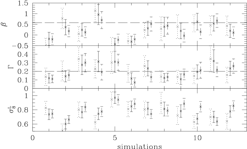
Figure 1: The estimation of parameters in $N$-body simulations. Horizontal axis indicate the different realization of mock catalog. The true values in the simulations are shown by long-dashed horizontal lines for $\beta$ and $\Gamma$. The dotted lines are for $M=100$, solid lines for $M=150$, and dashed lines for $M=200$.

Figure 2: Likelihood function of LCRS data. Upper panel: Three-dimensional likelihood function. Four sections of fixed $\Gamma$ are plotted as a contour map, in which $1\sigma$, $2\sigma$, and $3\sigma$ confidence levels are shown. Lower panel: Marginalized likelihood functions of each parameter. Number of KL modes used in likelihood analysis is varied. Dotted lines are for $M=100$, solid lines for $M=150$, and dashed lines for $M=200$.

Table 1: Best fit models from the projected likelihood functions with $M=150$. Error ranges correspond to 1 $\sigma$ of the likelihood functions.

Sample	$\beta$	$\Gamma$	$\sigma_{8}^{\rm L}$
North	$0.24\pm 0.42$	$0.16\pm 0.11$	$0.77\pm 0.09$
South	$0.36\pm 0.37$	$0.17\pm 0.08$	$0.81\pm 0.09$
Combined	$0.30\pm 0.39$	$0.16\pm 0.10$	$0.79\pm 0.08$

References

- Broadhurst et al. (1990) Broadhurst,T.J, Ellis, R.S., Koo, D.C. & Szalay, A.S. 1990, Nature, 343, 726.
- Feldman, Kaiser, & Peacock (1994) Feldman, H.A., Kaiser, N., & Peacock, J.A. 1994, ApJ, 426, 23.
- Fischer et al. (1993) Fisher, K.B, Davis, M., Strauss, M.A., Yahil, A., & Huchra, J.P. 1993, ApJ, 402, 42.
- Hoffman (1999) Hoffman, Y. 1999, in Cosmic Flows. Towards an Understanding of Large-Scale Structure, Workshop Victoria B.C., July 1999, eds. S. Courteau, M. Strauss, and J. Willick (astro-ph/9909158)
- Landy et al. (1996) Landy, S.D., Shectman, S.A., Lin H., Kirschner, R.P., Oemler, A.A. & Tucker, D. 1996, ApJ, 456, L1.
- Lin et al. (1996) Lin, H., Kirshner, R. P., Shectman, S. A., Landy, S. D., Oemler, A., Tucker, D. L., & Schechter, P. L. 1996, ApJ, 471, 617
- Matsubara et al. (1999) Matsubara, T., Szalay, A. S. & Landy, S. D. 2000, in progress.
- Park et al. (1994) Park, C., Vogeley, M. S., Geller, M. J., & Huchra, J. P. 1994, ApJ, 431, 569.
- Shectman et al. (1996) Shectman, S.A., Landy, S.A., Oemler, A., Tucker, D.,Lin, H., Kirschner, R.L. & Schechter, P.L. 1996, ApJS, 470, 172.
- Szalay et al. (1998) Szalay, A. S., Matsubara, T. & Landy, S. D. 1998, ApJ, 498, L1
- Tegmark et al. (1998) Tegmark, M., Hamilton, A.J.S., Strauss, M., Vogeley, M.S. & Szalay, A.S. 1998, ApJ, 499, 555.
- Vogeley & Szalay (1996) Vogeley, M. S. & Szalay, A. S. 1996, ApJ, 465, 34.