Thermal synchrotron radiation and its Comptonization
in compact X-ray sources

Abstract

We investigate the process of synchrotron radiation from thermal electrons at semi-relativistic and relativistic temperatures. We find an analytic expression for the emission coefficient for random magnetic fields with an accuracy significantly higher than of those derived previously. We also present analytic approximations to the synchrotron turnover frequency, treat Comptonization of self-absorbed synchrotron radiation, and give simple expressions for the spectral shape and the emitted power. We also consider modifications of the above results by bremsstrahlung.

We then study the importance of Comptonization of thermal synchrotron radiation in compact X-ray sources. We first consider emission from hot accretion flows and active coronae above optically-thick accretion discs in black-hole binaries and AGNs. We find that for plausible values of the magnetic field strength, this radiative process is negligible in luminous sources, except for those with hardest X-ray spectra and stellar masses. Increasing the black-hole mass results in a further reduction of the maximum Eddington ratio due to this process. Then, X-ray spectra of intermediate-luminosity sources, e.g., low-luminosity AGNs, can be explained by synchrotron Comptonization only if they come from hot accretion flows, and X-ray spectra of very weak sources are always dominated by bremsstrahlung. On the other hand, synchrotron Comptonization can account for power-law X-ray spectra observed in the low states of sources around weakly-magnetized neutron stars.

1 Introduction

The theory of cyclotron and synchrotron radiation is a well established part of physics. However, there still remain uncertainties about the accuracy and the range of applicability of some analytic formulae describing the emission. One important example of such uncertainties concerns the spectra of synchrotron emission from mildly-relativistic and relativistic thermal plasma, in which case numerous studies devoted to this field, e.g., Jones & Hardee (1979), Petrosian (1981, hereafter P81), Takahara & Tsuruta (1982), Petrosian & McTiernan (1983), Robinson & Melrose (1984), Mahadevan, Narayan & Yi (1996, hereafter MNY96), yielded results not entirely consistent with each other.

Precise determination of spectra from the thermal synchrotron process is of key significance for studies of emission from accretion flows onto black holes and neutron stars. Although direct, optically-thin, thermal synchrotron emission is rarely observable, accurate optically-thin spectra are necessary to determine the turnover frequency, below which the plasma becomes optically-thick. The resulting partially-absorbed spectrum is then observable in some cases. Furthermore, photons from that spectrum provide a supply of seed photons for Comptonization in the plasma, which process gives rise to observable power-law spectra with high-energy cutoffs. On the other hand, blackbody radiation emitted by optically-thick accretion discs and other forms of optically-thick matter may constitute a competing supply of seed photons. In addition, bremsstrahlung radiation is always emitted by a hot plasma.

In this work, we first consider formulae for the synchrotron emission coefficient of a thermal plasma (Section 2). We clarify the accuracy and the range of applicability of previously derived formulae as well as propose our own expressions. We concentrate on mildly relativistic and relativistic plasmas, as exhaustive studies of non-relativistic thermal cyclotron emission exist (Chanmugam et al. 1989 and references therein). We then calculate the turnover frequency and consider effects of bremsstrahlung emission and self-absorption. Second, we investigate Comptonization of the synchrotron radiation (hereafter abbreviated as the CS process) and present convenient formulae for the resulting spectra and luminosities (Section 3). In Section 4, we apply our results to two main geometries of accretion flows onto a black hole: a hot, two-temperature, optically thin disc, and active regions above a cold disc (i.e., a patchy corona). Those two models, for various plausible prescriptions for the magnetic field strength, are then compared with spectral data from black-hole binaries and AGNs. Finally, in Section 5, we study the importance of the CS proces for formation of spectra of accreting neutron stars with weak/moderate magnetic fields.

2 Synchrotron radiation from thermal plasmas

2.1 Emission of a single electron

Let us consider an electron (with charge $e$) moving in a uniform magnetic field, $\mn@boldsymbol{B}$, at a velocity, $\mn@boldsymbol{\beta}\equiv\mn@boldsymbol{v}/c$. Let $\xi$ be the angle between $\mn@boldsymbol{v}$ and $\mn@boldsymbol{B}$, and $\vartheta$ be the angle between $\mn@boldsymbol{B}$ and the direction towards the observer. Then, the cyclo-synchrotron power per unit frequency and unit solid angle in the observer frame and in cgs units is given by (e.g. Bekefi 1966; Pacholczyk 1970)

$$\eta_{\nu}\equiv\hbox to0.0pt{$\displaystyle\frac{{\rm d}W}{{\rm d}\nu\,{\rm d}\Omega\,{\rm d}t}(\vartheta,\xi,\gamma)=\frac{2\pi e^{2}\nu^{2}}{c}\times$\hss}$$ (1)

$$\sum_{n=1}^{\infty}\delta(y_{n})\left[\left(\frac{\cos\vartheta-\beta\cos\xi}{\sin\vartheta}\right)^{2}J^{2}_{n}(z)+\beta^{2}\sin^{2}\xi J^{\prime 2}_{n}(z)\right],$$

where

$$y_{n}\equiv\frac{n\nu_{\rm c}}{\gamma}-\nu(1-\beta\cos\xi\cos\vartheta),\,\,z\equiv\frac{\nu\gamma\beta\sin\vartheta\sin\xi}{\nu_{\rm c}},$$ (2)

$\nu_{\rm c}\equiv eB/2\pi m_{\rm e}c$ is the cyclotron frequency, $\gamma=(1-\beta^{2})^{-1/2}$ is the Lorentz factor, $J_{n}$ is a Bessel function of order $n$, and $m_{\rm e}$ is the electron mass.

Note that an additional factor of $(1-\beta\mu\cos\vartheta)^{-1}$ due to the Doppler effect should have appeared in the formal derivation of equation (1). However, this term disappears in the case of an electron moving chaotically, as, e.g., in a thermal plasma. For detailed discussion, see Scheuer (1968), Rybicki & Lightman (1979, section 6.7), Pacholczyk (1970, section 3) and references in these works.

2.2 Synchrotron emission coefficient in a thermal plasma

The emission coefficient, $j_{\nu}(\vartheta)$, of a thermal plasma at a temperature, $T$, and with a uniform magnetic field, $\mn@boldsymbol{B}$, can be obtained by integrating the rate of equation (1) over a relativistic Maxwellian electron distribution,

$$n_{\rm e}(\gamma)=\frac{n_{\rm e}}{\Theta}{\gamma(\gamma^{2}-1)^{1/2}\over K_{2}(1/\Theta)}\exp\left(-{\gamma\over\Theta}\right),$$ (3)

where $\Theta\equiv kT/m_{\rm e}c^{2}$ is the dimensionless plasma temperature, and $n_{\rm e}$ is the electron density. $K_{2}$ is a modified Bessel function, which can be approximated by

$$K_{2}\left(1\over\Theta\right)\approx$$ (4)

$$\cases{\left(\pi\Theta\over 2\right)^{1/2}\left(1+{15\Theta\over 8}+{105\Theta^{2}\over 128}-0.203\Theta^{3}\right){\rm e}^{-1/\Theta},&$\Theta\leq 0.65$;\cr 2\Theta^{2}-{1\over 2}+{\ln(2\Theta)+3/4-\gamma_{\rm E}\over 8\Theta^{2}}+{\ln(2\Theta)+0.95\over 96\Theta^{4}},&$\Theta\geq 0.65$,\cr}$$

where $\gamma_{\rm E}\approx 0.5772$ is Euler’s constant and the last coefficients in the series have been adjusted to achieve a relative error $\leq 0.0008$.

The integral for the emission coefficient is then,

$$j_{\nu}(\vartheta)=\int_{1}^{\infty}{\rm d}\gamma\,{1\over 2}n_{\rm e}(\gamma)\int_{-1}^{1}{\rm d}\mu\,\eta_{\nu}(\vartheta,\mu,\gamma),$$ (5)

where $\mu=\cos\xi$. This integration is relatively difficult to carry out due to the complicated form of the integrand and the presence of $J_{n}$ in $\eta_{\nu}$. In particular, standard numerical methods of computing $J_{n}$ become very inefficient for $n\gg 1$. P81 obtained an approximate solution by replacing the summation over $n$ by integration over $\nu$ in equation (1) and then using the principal term of an asymptotic expansion of $J_{n}(z)$, where $0\leq z\leq n\beta<n$ [see equation (9.3.7) of Abramowitz & Stegun (1970, hereafter AS70)]. The region of validity of that approximation of $J_{n}$ is given by $\gamma^{2}\ll\nu/\nu_{\rm c}$. The integration over $\mu$ and $\gamma$ by the method of the steepest descent with some additional approximations yields

$$j_{\nu}(\vartheta)=\frac{2^{1/2}\pi e^{2}n_{\rm e}\nu}{3c\,K_{2}(1/\Theta)}\exp\left[-\left({9v\over 2\sin\vartheta}\right)^{1/3}\right].$$ (6)

where $v\equiv\nu/\nu_{\rm c}\Theta^{2}$. We see that the emission coefficient becomes very small both at large frequencies, and at viewing angles, $\vartheta$, significantly different from $\pi/2$.

We note that equation (26) in P81, which corresponds to the formula (6), is too small by a factor of 2 due to the adopted normalization of the electron distribution [equation (23) in P81] being also twice too small. On the other hand, Takahara & Tsuruta (1982) obtain a formula [equation (2.9) in their paper] for the absorption coefficient for the perpendicular polarization of synchrotron radiation, $\alpha_{\nu}^{\perp}$, which agrees with our expression (6) for the emission coefficient at $\vartheta=\pi/2$. (They also compute the coefficient for the parallel polarization, $\alpha_{\nu}^{\parallel}$, which, however, is negligibly small compared to the dominant coefficient of the perpendicular polarization.) We note that the relation between the absorption and emission coefficients is given by Kirchhoff’s law, which, in the case of polarized radiation, contains the source function for each polarization separately, i.e., $B^{\parallel}_{\nu}=B^{\perp}_{\nu}=B_{\nu}/2$ (see, e.g. Chanmugam et al. 1989). The coefficients for polarized radiation are then related to the coefficients including both polarizations by $j_{\nu}=j^{\parallel}_{\nu}+j^{\perp}_{\nu}$, $\alpha_{\nu}=({\alpha}^{\parallel}_{\nu}+{\alpha}^{\perp}_{\nu})/2$. We also note that the emission coefficient computed by Jones & Hardee (1979) for $\Theta\gg 1$ is larger than the corresponding limit of equation (6) by a factor of $2^{1/2}$, which discrepancy we have not been able to explain.

In our numerical calculations, we used an approximation of $J_{n}(z)$ in terms of the Airy function [equation (9.3.6) in AS70], which maximum relative error is $\sim 0.08$ at $n=1$, $z=0$, but it rapidly decreases for larger values of $n$, $z$. If the argument of the Airy function is $<2.25$, we approximate it by its power series [equation (10.4.3) in AS70] up to the 13th power. Otherwise, we use the approximation to $J_{n}$ of P81 described above, in which case the maximum error is $\sim 0.02$. Typical relative accuracy of the resulting approximation to $J_{n}$ is then $<0.01$. The accuracy can be further increased by adding the first-order correction to the principal term of the asymptotic expansion of $J_{n}$, see equation (9.3.7) in AS70. The derivative, $J^{\prime}_{n}$, is calculated with the second expression in equation (9.1.30) of AS70. Note that the above method is more accurate, but also more complicated, than a related method given by Wind & Hill (1971).

Figure 1: (a) Contour plots of the ratio of the approximated emission coefficient of equation (6) to the exact numerical value (at $\vartheta=\pi/2$). (b) The same for equations (2.2)-(10).

We have tested the accuracy of formula (6) compared to the results of numerical integration (which themselves are in a very good agreement with numerical results tabulated for $\Theta\la 0.1$ by Chanmugam et al. 1989) of equation (5) at $\vartheta=\pi/2$ for $10\leq\nu/\nu_{\rm c}\leq 1000$ and $10^{-3}\leq\Theta\leq 10$. These ranges include parameters most relevant for compact sources (e.g. Takahara & Tsuruta 1982; Zdziarski 1986, hereafter Z86; Narayan & Yi 1995, hereafter NY95), and we hereafter use them while testing other synchrotron rates. Figure 1a shows the results for $\Theta>0.02$. We see that equation (6) overestimates the actual value of $j_{\nu}$ by orders of magnitude at low values of $\Theta$, and should not be used at all for $\Theta\la 0.1$. The relative accuracy strongly depends on $\Theta$ (being best at $\Theta\sim 0.4$) and it improves with increasing $\nu/\nu_{\rm c}$. In the relativistic limit, $\Theta\gg 1$, the accuracy of formula (6) depends on $v$ only.

We thus see that the accuracy of the emission coefficient (6) is not satisfactory for detailed modelling of astrophysical plasmas, as also found by MNY96. We suggest using a significantly more accurate expression [eq. (11) of P81 with additional approximations of eq. (25) of P81 and eq. (20) of Petrosian & McTiernan (1983)],

$$j_{\nu}(\vartheta)=\frac{\pi e^{2}}{2\,c}\left(\nu\nu_{\rm c}\right)^{1/2}{\cal X}(\gamma_{0})n_{\rm e}(\gamma_{0})\left(1+2{\cot^{2}\vartheta\over\gamma_{0}^{2}}\right)$$

$$\qquad\times\left[1-(1-\gamma_{0}^{-2})\cos^{2}\vartheta\right]^{1/4}{\cal Z}(\vartheta,\gamma_{0}).$$ (7)

Here

$${\cal Z}(\vartheta,\gamma)=\left[\frac{t\exp{\left[(1+t^{2})^{-{1\over 2}}\right]}}{1+(1+t^{2})^{1\over 2}}\right]^{2n}\!,\,\,t\equiv(\gamma^{2}-1)^{1\over 2}\sin\vartheta,$$ (8)

$$n\equiv\frac{\nu(1+t^{2})}{\nu_{\rm c}\gamma},\quad{\cal X}(\gamma)=\cases{\left[\frac{2\Theta\left(\gamma^{2}-1\right)}{\gamma\left(3\gamma^{2}-1\right)}\right]^{1/2},&$\Theta\la 0.08$;\cr\left(\frac{2\Theta}{3\gamma}\right)^{1/2},&$\Theta\ga 0.08$,}$$ (9)

and

$$\gamma_{0}=\cases{\left[1+\left(\frac{2\,\nu\Theta}{\nu_{\rm c}}\right)\left(1+\frac{9\,\nu\Theta\sin^{2}\vartheta}{2\,\nu_{\rm c}}\right)^{-{1\over 3}}\right]^{1\over 2}\!,&$\Theta\la 0.08$;\cr\left[1+\left(\frac{4\,\nu\Theta}{3\,\nu_{\rm c}\sin\vartheta}\right)^{2\over 3}\right]^{1\over 2},&$\Theta\ga 0.08$,}$$ (10)

where $\gamma_{0}$ is the Lorentz factor of the saddle point of the integral (5) over $\gamma$ (i.e. of those thermal electrons that contribute most to the emission at $\nu$), corresponding to the minimum of $n_{\rm e}(\gamma){\cal Z}(\vartheta,\gamma)/\gamma$. Note that approximations (9) and (10) have a small discontinuity at $\Theta\simeq 0.08$.

Figure 1b shows the relative accuracy of the approximation of equations (2.2)-(10). We see it is much more accurate than expression (6) throughout the test range, with the minimum relative error at $0.01\la\Theta\la 0.2$. Also, the relative accuracy of this approximation varies with $\Theta$ and $\nu/\nu_{\rm c}$ much slower than that of equation (6). At $\Theta\sim 10^{-3}$ the approximation (2.2)-(10) matches well the nonrelativistic emission coefficient given by equations (14)-(15) of Trubnikov (1958).

Our expression (2.2)-(10) can be compared with that of Robinson & Melrose (1984), who have also used a method based on that of P81 with accuracy improved with respect to that paper. We have found that their expression, in the form of Dulk (1985) and with the non-relativistic Maxwellian replaced by the relativistic one, is slightly more accurate, but also more complicated, than expression (2.2)-(10). We also note that a relativistic generalization of the results of Robinson & Melrose (1984) by Hartmann, Woosley & Arons (1988) appears incorrect. Namely, their expression (B1) should be multiplied by a factor $2\pi(\gamma^{2}_{0}-1)^{-1/2}$ (in their notation).

2.3 Angle-averaged emission coefficient

The emission coefficients derived above are appropriate for a plasma in a uniform magnetic field. However, in typical astrophysical conditions, we expect either to deal with emission from regions where magnetic fields are chaotic or to observe radiation being a sum of contributions from a number of regions with different orientations of magnetic field. Therefore, we would like to find the emission coefficient averaged over magnetic field directions (or, equivalently, over the viewing angle), $\bar{j}_{\nu}=\epsilon_{\nu}/4\pi$, where $\epsilon_{\nu}$ is the emitted power per unit volume and frequency, and

$$\bar{j}_{\nu}={1\over{4\pi}}\int j_{\nu}(\vartheta){\rm d}\Omega={1\over 2}\int j_{\nu}(\vartheta)\sin\vartheta\;{\rm d}\vartheta.$$ (11)

To obtain an expression for $\bar{j}_{\nu}$, we integrate equation (2.2) over $\vartheta$ using the method of the steepest descent with the saddle point at $\vartheta=\pi/2$. Here, we treat ${\cal Z}$ as the fast varying (with $\vartheta$) part of the integrand (2.2). The resulting expression is,

$$\bar{j}_{\nu}=\frac{\pi^{3\over 2}e^{2}\left(\nu\nu_{\rm c}\right)^{1\over 2}n_{\rm e}(\gamma_{0}){\cal Z}(\vartheta,\gamma_{0}){\cal X}(\gamma_{0})}{2^{3\over 2}c}\left|\partial^{2}\ln{\cal Z}(\vartheta,\gamma_{0})\over\partial\vartheta^{2}\right|^{-{1\over 2}}$$ (12)

to be evaluated at $\vartheta=\pi/2$.

On the other hand, the asymptotic emission coefficient (6) can be integrated over $\vartheta$, as done by MNY96. This yields,

$$\bar{j}_{\nu}={2^{1/6}\pi^{3/2}e^{2}n_{\rm e}\nu\over 3^{5/6}cK_{2}(1/\Theta)v^{1/6}}a(\Theta,v)\exp\left[-\left(9v\over 2\right)^{1/3}\right],$$ (13)

where the correction factor, $a$, represents the ratio of the exact emission coefficient to that obtained by integration of equation (6). This factor can be calculated from the ratio of equations (33) to (31) in MNY96 with fitting coefficients of their Table 1.

We have tested the accuracy of the formulae (12) and (13), the latter both with and without the tabulated corrections, again in the range $10^{-3}\leq\Theta\leq 10$ and $10\leq\nu/\nu_{\rm c}\leq 1000$. Figure 2a shows the relative error of equation (12). We see that the relative error is typically $\la 30$ per cent except for $\Theta>1$ with the best accuracy at $0.02\la\Theta\la 0.4$.

Figure 2: (a) Contour plots of the ratio of the approximated emission coefficient (12) to the correct numerical value. (b) The same for equation (13) with $a\equiv 1$.

The expression (13) with the tabulated corrections of MNY96 matches very well the numerical results (the difference is less than a few per cent), with the exception of the case of $\Theta=0.084$, where the corrections in Table 1 of MNY96 appear misprinted as the obtained values are a few times too small and the error increases with frequency.

The accuracy of formula (13) with $a\equiv 1$ is shown in Figure 2b. We see that it provides an estimate correct within a factor of $\sim 3$ or better only for $\Theta>0.1$ and the best accuracy is obtained at $\Theta\sim 0.6$ This formula strongly overestimates the correct result for $\Theta\la 0.1$. At relativistic temperatures, $\Theta\gg 1$, the relative accuracy of equation (13) with $a\equiv 1$ depends on $v$ only. It underestimates somewhat the actual emission coefficient, and its integration over $\nu$ yields a value of the total emitted power too low by a factor of $3^{1/2}35\pi/2^{8}\simeq 0.744$ with respect to the actual power,

$$\epsilon=16\Theta^{2}n_{\rm e}\sigma_{\rm T}c{B^{2}\over 8\pi},\quad\Theta\gg 1,$$ (14)

where $\sigma_{\rm T}$ is the Thomson cross section. Then, equation (13) with $a\equiv 1$ and divided by 0.744 represents an approximation to the ultra-relativistic thermal synchrotron emission coefficient satisfying the total-power constraint (14).

2.4 Synchrotron self-absorption

The synchrotron radiation is self-absorbed by electrons up to the turnover frequency, $\nu_{\rm t}$, above which the plasma becomes optically thin to the synchrotron radiation, i.e.,

$$\tau=\alpha_{\nu_{\rm{}_{t}}}R=1,$$ (15)

where $R$ is the characteristic size of the plasma. Below $\nu_{\rm t}$, the observed spectrum has the blackbody form, typically in the Rayleigh-Jeans limit. In this limit and averaging over angles, Kirchhoff’s law implies,

$${\bar{j}_{\nu_{\rm t}}\over 2\nu_{\rm t}^{2}m_{\rm e}\Theta}R=1.$$ (16)

This can be solved numerically. On the other hand, Zdziarski et al. (1998) give the solution using equation (13),

$${\nu_{\rm t}\over\Theta^{2}\nu_{\rm c}}=\frac{343}{36}\ln^{3}{C\over\ln{C\over\ln{C\over\dots}}},\,\,\,C=\frac{3}{7\Theta}\left[\pi\tau_{\rm T}a\exp(1/\Theta)\over 3\alpha_{\rm f}x_{\rm c}\right]^{2\over 7}\!,$$ (17)

where $x_{\rm c}\equiv h\nu_{\rm c}/m_{\rm e}c^{2}$ is a dimensionless cyclotron frequency, $\tau_{\rm T}=n_{\rm e}\sigma_{\rm T}R$ is the Thomson optical depth of the plasma, and $\alpha_{\rm f}$ is the fine-structure constant. Note that $\nu_{\rm t}$ depends on $n_{\rm e}$ and $R$ only through their product, or equivalently, $\tau_{\rm T}$. Typically, the correction factor, $a$, is a slowly-varying function of frequency (MNY96) and then equation (17) for $\nu_{\rm t}$ is explicit. We also see that the dependence of $\nu_{\rm t}$ on $a$ is only logarithmic, and thus the accuracy of determining the synchrotron emission coefficient only weakly affects the turnover frequency.

Mahadevan (1997) used a slightly different method of determining $\nu_{\rm t}$. Namely, he equated the total flux of the Rayleigh-Jeans emission to that in the optically-thin synchrotron one. This corresponds to setting the right-hand side of equation (16) to 3/4 instead of 1, which changes slightly the resulting value of $\nu_{\rm t}$ as compared to equation (17).

We have compared the approximated formula (17) with $a\equiv 1$ with results of numerical calculations. It turns out that the error of equation (17) is almost independent of the values of the parameters other then $\Theta$. Figure 3 compares the results of the two methods in the temperature range $0.03\leq\Theta\leq 1$ for a source with $\tau_{\rm T}=1$, $R=10^{7}\,$cm and $B=10^{6}\,$G. (In this parameter range, the effect of bremsstrahlung can be neglected, see below.) We see that for $0.1\la\Theta\la 1$ the discrepancy does not exceed 20 per cent but grows rapidly for lower temperatures. We have also found a power-law approximation for $x_{\rm t}\equiv h\nu_{\rm t}/m_{\rm e}c^{2}$ as

$$x_{\rm t}\approx 2.6\times 10^{-6}\left(\Theta\over 0.2\right)^{0.95}\tau_{\rm T}^{0.05}\left(B\over 10^{6}\,{\rm G}\right)^{0.91},$$ (18)

which is accurate to $\la 30$ per cent for $0.05\la\Theta\la 0.4$, $0.3\la\tau_{\rm T}\la 3$, $10\,{\rm G}\la B\la 10^{8}$ G. Typical values of $x_{\rm t}/x_{\rm c}$ at mildly-relativistic temperatures are in the range of 10–$10^{3}$.

Figure 3: The ratio of the turnover frequency calculated from equation (17) with $a\equiv 1$ to the accurate numerical result as a function of temperature.

2.5 Effect of bremsstrahlung on the turnover frequency

We note that the above formulae for the turnover frequency do not take into account bremsstrahlung emission and self-absorption. However, for some combinations of $\Theta$, $n_{\rm e}$ and $B$, bremsstrahlung emission can be comparable to or stronger than the synchrotron one and then the turnover frequency determined neglecting bremsstrahlung will be incorrect. Then, the absorption coefficient, $\alpha_{\nu_{\rm t}}$, should include a contribution from bremsstrahlung, $\alpha^{\rm ff}_{\nu}$. Note that since $\alpha^{\rm ff}_{\nu}\propto n_{\rm e}^{2}R$, $\nu_{\rm t}$ is no more solely a function of $\tau_{\rm T}$ whenever bremsstrahlung is important.

The effect of bremsstrahlung on the turnover frequency can be checked by computing $\nu_{\rm t}$ without taking into account bremsstrahlung, and then computing the emission coefficient, $\bar{j}_{\nu_{\rm{}_{t}}}$, including both processes. As long as $\bar{j}_{\nu_{\rm{}_{t}}}\gg j^{\rm ff}_{\nu_{\rm{}_{t}}}$, equations in Section 2.4 can be used. We hereafter use formulae for the free-free emission coefficient of Svensson (1984).

Figure 4: Example dependences of the turnover frequency on (a) temperature and (b) magnetic field strength. The dot-dashed and dashed curves give $\nu_{\rm t}$ calculated with the analytic approximation of equation (17), and numerically using equation (16), respectively, with bremsstrahlung neglected in both cases. The solid curves give the numerical results with bremsstrahlung taken into account.

We have calculated the turnover frequency as a function of $\Theta$ and $B$ for the remaining parameters fixed, see Figures 4a, b, respectively. As expected, $\nu_{\rm t}$ is determined mostly by bremsstrahlung at low temperatures and weak magnetic fields. However, though bremsstrahlung can have a negligible effect on the value of $\nu_{\rm t}$, the total emitted power can still be dominated by it, see Section 4 below, and, e.g. Figure 3 in Z86. On the other hand, if bremsstrahlung self-absorption dominates over the synchrotron one, bremsstrahlung emission will also dominate over the CS emission, except in the case of spectra of the latter emission being harder than the bremsstrahlung spectrum.

3 Comptonization of synchrotron photons

Synchrotron photons produced in a plasma will, in general, be Compton scattered by the plasma electrons. In the case of a thermal plasma, the synchrotron spectrum is usually self-absorbed up to a high value of $\nu/\nu_{\rm c}$ (Section 2.4). In that case, the self-absorbed synchrotron spectrum is rather narrow, consisting of a hard Rayleigh-Jeans spectrum at $\nu\la\nu_{\rm t}$ (in which regime scattering can be neglected, $\tau\gg\tau_{\rm T}$, $\tau\gg 1$), and a fast-declining tail of the optically-thin synchrotron spectrum at $\nu\ga\nu_{\rm t}\gg\nu_{\rm c}$ (where absorption can be neglected, $\tau\ll\tau_{\rm T}$, $\tau\ll 1$). Photons in that spectrum then serve as seed photons for Comptonization. For that process, it is usually sufficient to treat the self-absorbed synchrotron photons as monochromatic at $\nu_{\rm t}$ (see, e.g., Monte Carlo simulations in Z86). Also, for magnetic fields, $B\la 10^{9}$ G, and electron temperatures, $kT\ga 10$ keV, expected in compact sources, $h\nu_{\rm t}\ll kT$, and photons at $\nu\sim\nu_{\rm t}$ gain energy in the scattering process.

To treat thermal Comptonization, we use the method of Zdziarski (1985, hereafter Z85), as applied to thermal synchrotron sources in Z86. This method gives an approximate form of Comptonized spectra, reproducing relatively accurately the energy spectral index, $\alpha$, and the total power in the scattered spectrum (see comparison with Monte Carlo results in Z86). On the other hand, it gives a relatively inaccurate shape of the high-energy cutoff of the scattered spectrum (see, e.g., Poutanen & Svensson 1996), which, however, is of negligible importance for our applications.

We consider a homogeneous and isotropic source characterized by $\tau_{\rm T}$, $\Theta$ and $B$. The flux in scattered photons can be approximated as a sum of a cut-off power law and a Wien component,

$$F_{\rm C}(x)=N_{\rm P}\left(\frac{x}{\Theta}\right)^{-\alpha}{\rm e}^{-x/\Theta}+N_{\rm W}\left(\frac{x}{\Theta}\right)^{3}{\rm e}^{-x/\Theta},$$ (19)

where $x\equiv h\nu/m_{\rm e}c^{2}$ is a dimensionless photon energy, and $N_{\rm P}$, $N_{\rm W}$ are normalizations of the power-law and Wien components, respectively.

For $\tau_{\rm T}\la 2$, $\alpha$ can be approximately given by,

$$\alpha=-\frac{\ln P_{\rm sc}}{\ln A},\qquad A\equiv 1+\left\langle\frac{\Delta\nu}{\nu}\right\rangle\approx 1+4\Theta+16\Theta^{2},$$ (20)

where $A$ is the average photon energy amplification per scattering and $P_{\rm sc}$ is the scattering probability averaged over the source volume. Note that $\alpha>0$ in general. In spherical geometry (Osterbrock 1974),

$$P_{\rm sc}=1-\frac{3}{8\tau_{\rm T}^{3}}\left[2\tau_{\rm T}^{2}-1+{\rm e}^{-2\tau_{\rm T}}(2\tau_{\rm T}+1)\right]$$

$$\qquad\rightarrow\cases{{3\tau_{\rm T}\over 4},&$\tau_{\rm T}\ll 1$;\cr 1-{3\over 4\tau_{\rm T}},&$\tau_{\rm T}\gg 1$,\cr}$$ (21)

where $\tau_{\rm T}$ is the Thomson optical depth along the radius. We have found a power-law approximation to $\alpha(\tau_{\rm T},\Theta)$ valid at $0.5\la\tau_{\rm T}\la 2$ and $\Theta\la 0.4$,

$$\alpha\approx{3\over 19}{1\over\tau_{\rm T}^{4/5}\Theta}.$$ (22)

See Zdziarski et al. (1994) for $P_{\rm sc}$ in the slab geometry. In general, different prescriptions for $\alpha(\tau,\Theta)$ can be used, e.g., in order to account for a different geometry or to increase the accuracy, without affecting the validity of the results presented below in this section. On the other hand, some equations in Section 4 utilize equation (22), and using a different $\alpha(\tau,\Theta)$ would somewhat change those formulae.

Note that at $\tau_{\rm T}\ll 1$, scattering profiles corresponding to subsequent scatterings are visible in the Compton spectrum, and a power law is no longer a good approximation to the shape of the spectrum below the cutoff (e.g., Fig. 2b in Z86). Still, the power-law description presented here gives the shape averaged over the scattering orders, and an integral over that approximate form gives a fair approximation to the total luminosity (see, e.g., Monte Carlo simulations in Z86). On the other hand, at $\tau_{\rm T}\ga 2$–3, Comptonization can be described by means of a kinetic, Fokker-Planck, equation (Sunyaev & Titarchuk 1980; see e.g. Lightman & Zdziarski 1987 for relativistic and low-$\tau_{\rm T}$ corrections). The two solutions can be matched at $\tau_{\rm T}\sim 2$ (Z85). The remaining results presented in this Section can still be used at $\tau_{\rm T}\ga 2$–3, except for a different prescription for $\alpha$. In particular, the ratio of $N_{\rm W}/N_{\rm P}$ given by Z85,

$$\frac{N_{\rm W}}{N_{\rm P}}=\frac{\Gamma(\alpha)}{\Gamma(2\alpha+3)}P_{\rm sc},$$ (23)

where $\Gamma$ is Euler’s gamma function, and which uses a result of Sunyev & Titarchuk (1980), is a good approximation in both the optically-thin and optically-thick regimes (see, e.g., comparison with Monte Carlo results in Z86).

We need then to normalize the flux in the Compton-scattered spectrum, $F_{\rm C}(x)$, with respect to that in the Rayleigh-Jeans spectrum, $F_{\rm RJ}(x)$. In general, the self-absorbed synchrotron spectrum at its peak around $x_{\rm t}$ ($\equiv h\nu_{\rm t}/m_{\rm e}c^{2}$) is somewhat above an extrapolation of the power-law component of the Compton spectrum, $F_{\rm C}(x)$ (which follows from photon conservation, Z85). Z86 finds the following phenomenological relation providing a good approximation to the relative normalization,

$$F_{\rm C}(x_{\rm t})=\varphi F_{\rm RJ}(x_{\rm t}),\quad\varphi(\Theta)\approx\frac{1+(2\Theta)^{2}}{1+10(2\Theta)^{2}}.$$ (24)

This is valid for $x_{\rm t}\ll\Theta$, which condition we assume hereafter. The flux of the Rayleigh-Jeans spectrum is given by,

$$F_{\rm RJ}(x)=\pi I_{\rm RJ}(x),\quad I_{RJ}(x)=\frac{2m_{\rm e}c^{3}\Theta}{\lambda_{\rm C}^{3}}x^{2},$$ (25)

where $I_{\rm RJ}$ is the specific intensity and $\lambda_{\rm C}\simeq 2.426\times 10^{-10}$ cm is the electron Compton wavelength. Then,

$$N_{\rm P}=\pi\varphi I_{RJ}(x_{\rm t})(x_{\rm t}/\Theta)^{\alpha}.$$ (26)

The luminosity due to the CS emission is then given by,

$$L_{\rm CS}={\cal A}\left[\int_{0}^{x_{\rm t}}{\rm d}x\;F_{\rm RJ}(x)+\int^{\infty}_{x_{\rm t}}{\rm d}x\;F_{\rm C}(x)\right].$$ (27)

where ${\cal A}$ is the source area, and which can be integrated to,

$$L_{\rm CS}={\cal A}{2\pi m_{\rm e}c^{3}\Theta x_{\rm t}^{3}\over 3\lambda_{\rm C}^{3}}\left\{1+3\varphi\left(x_{\rm t}\over\Theta\right)^{\alpha-1}\times\right.$$

$$\left.\qquad\left[\Gamma\left(1-\alpha,{x_{\rm t}\over\Theta}\right)+\frac{6\Gamma(\alpha)P_{\rm sc}}{\Gamma(2\alpha+3)}\right]\right\},$$ (28)

where the incomplete gamma function is well approximated for $x_{\rm t}\ll\Theta$ by,

$$\Gamma\left(1-\alpha,{x_{\rm t}\over\Theta}\right)\simeq$$

$$\cases{\ln{\Theta\over x_{\rm t}}-\gamma_{\rm E},&$|\alpha-1|<10^{-3}$;\cr{\Theta\over x_{\rm t}}-\ln{\Theta\over x_{\rm t}}-1+\gamma_{\rm E},&$|\alpha-2|<10^{-3}$;\cr{1\over\alpha-1}\left(\Theta\over x_{\rm t}\right)^{\alpha-1},&$\alpha>2.99$;\cr\Gamma(1-\alpha)-{(x_{\rm t}/\Theta)^{1-\alpha}\over 1-\alpha}+{(x_{\rm t}/\Theta)^{2-\alpha}\over 2-\alpha},&otherwise.}$$ (29)

At $x_{\rm t}/\Theta=0.01$, the maximum relative error of this approximation of $\sim 0.02$ occurs around $\alpha\simeq 3$. The relative error declines rapidly at lower values of $x_{\rm t}/\Theta$ and $\alpha$; e.g., it is $<0.001$ at $x_{\rm t}/\Theta=0.01$ and $\alpha\leq 2.9$, and $<0.002$ at $x_{\rm t}/\Theta=10^{-3}$ at any $\alpha$.

In an astrophysically important case of $\alpha\sim 0.4$–0.9 (e.g. Gierliński et al. 1997; Zdziarski, Lubiński & Smith 1999), the main contribution to the luminosity comes from the high-energy end of the spectrum, and the Wien component is relatively unimportant. Then, we obtain an approximation valid within a factor of $\la 2$ at $x_{\rm t}/\Theta\la 10^{-5}$,

$$L_{\rm CS}\approx{8\pi^{2}m_{\rm e}c^{3}R^{2}\over(1-\alpha)\lambda_{\rm C}^{3}}x_{\rm t}^{2+\alpha}\varphi\Theta^{2-\alpha},$$ (30)

where we assumed a spherical geometry. On the other hand, for soft spectra, with $\alpha\ga 1.1$, we get an approximation valid within $\sim 30$ per cent,

$$L_{\rm CS}\approx{8\pi^{2}m_{\rm e}c^{3}R^{2}\over 3\lambda_{\rm C}^{3}}\left(1+{3\varphi\over\alpha-1}\right)x_{\rm t}^{3}\Theta.$$ (31)

For order-of-magnitude estimates, we can then substitute $x_{\rm t}$ of equation (18) in equations (30)-(31). This yields $L_{\rm CS}\propto R^{2}\Theta^{3.78-0.11\alpha}B^{1.82+0.91\alpha}$ and $\propto R^{2}\Theta^{3.66}B^{2.73}$ for $0.4\la\alpha\la 0.9$ and $\alpha\ga 1.1$, respectively.

We stress that the above formulae for the Comptonization spectral shape and the corresponding expressions for the luminosity are mutually consistent. This is much preferable to computing Comptonization luminosity independently of its corresponding spectrum by multiplying the power in a self-absorbed synchrotron spectrum by an amplification factor of Comptonization (e.g. of Dermer, Liang & Canfield 1991), as often done in studies of advective flows.

4 Applications to accreting black holes

Figure 5 shows an example of the CS spectrum for parameters typical to low-luminosity AGNs. The spectrum has the Rayleigh-Jeans shape below the turnover frequency, it is a power law due to Comptonization above that frequency, and then it has a thermal high-energy cutoff. We also show the contribution due to Comptonized bremsstrahlung, which is moderately important for the chosen parameters. We have computed the latter spectrum by treating the spectrum of equation (19) as Green’s function for Comptonization and then integrating over the seed spectrum of optically-thin bremsstrahlung. The spectrum is computed assuming spherical geometry. More examples of spectra from magnetized plasmas are given, e.g. in Z86.

Figure 5: An example of the spectrum of a magnetized plasma, for $R=9\times 10^{13}$ cm, $B=2.2\times 10^{3}$ G, $\tau_{\rm T}=0.47$ and $\Theta=0.4$. The dotted, short-dashed and long-dashed curves represent spectra due to synchrotron emission, its Comptonization and Comptonized bremsstrahlung, respectively. The solid curve represents the sum of those components. This spectrum also represents a model of a hot accretion flow fitted to the X-ray data for NGC 4258 (bow-tie, Makishima et al. 1994), see Section 4.1.

For given $\Theta$, the Rayleigh-Jeans part of the spectrum is independent of $B$, and its spectral luminosity is $L_{\rm RJ}(\nu)\propto R^{2}$. On the other hand, the CS spectrum obeys $L_{\rm CS}(\nu)\propto R^{2}\nu_{\rm t}^{2+\alpha}$ [equation (26)], i.e., its normalization increases quickly with increasing $B$ via the dependence of the turnover frequency on $B$. When self-absorption is dominated by the synchrotron process, $\nu_{\rm t}$ is roughly $\propto B$ with no explicit dependence on $R$, see equation (18). The total luminosity, $L_{\rm CS}$, follows the same dependence if $\alpha\la 1$, see equation (30), and $L_{\rm CS}\propto R^{2}\nu_{\rm t}^{3}$ for $\alpha\ga 1$, see equation (31). The shape of the Comptonized bremsstrahlung spectrum is almost independent of $B$ (except for a very weak dependence of Comptonization on $\nu_{\rm t}$).

The bremsstrahlung luminosity can be constrained from below as

$$\frac{L_{\rm CB}}{L_{\rm E}}>1.2\times 10^{-6}\Theta^{1/2}\tau_{\rm T}^{2}r\approx 1.2\times 10^{-8}\alpha^{-5/2}\Theta^{-2}r,$$ (32)

where $r\equiv R/R_{\rm g}$, $R_{\rm g}\equiv GM/c^{2}$ is the gravitational radius, $L_{\rm E}\equiv 4\pi\mu_{\rm e}GMm_{\rm p}c/\sigma_{\rm T}\approx 1.5\times 10^{38}m$ erg s^-1 is the Eddington luminosity, $\mu_{\rm e}=2/(1+X)$ is the mean electron molecular weight, and $X$ ($\approx 0.7$) is the H mass fraction, and $m\equiv M/{\rm M}_{\odot}$. The right-hand-side expressions neglect Comptonization and relativistic corrections, which effects will increase the actual $L_{\rm CB}$. The last expression uses the approximation of equation (22) to $\alpha(\tau_{\rm T},\Theta)$. Note that $L_{\rm CB}$ represents a strict lower limit to the luminosity of a source with given $\tau_{\rm T}$, $\Theta$ and size. Thus, the luminosity of weak sources is dominated by $L_{\rm CB}$, with $L_{\rm CS}$ being negligible. Note, however, that usually the plasma parameters depend on luminosity, which dependence should be taken into account when determining the luminosity below which bremsstrahlung dominates.

Figure 6 shows some example dependences of the total $L$ on $B$ at $\Theta=0.05$–0.4 for $R=4\times 10^{7}$ cm and $4\times 10^{14}$ cm (corresponding to $\sim 30R_{\rm g}$ for 10M_⊙ and $10^{8}$M_⊙ black-hole mass, respectively). The flat parts at low values of $B$ correspond to the dominant bremsstrahlung, with its relative importance increasing with decreasing $\Theta$.

Figure 6: Example dependences of the plasma luminosity on $B$ for (a) $R=4\times 10^{7}$ cm and (b) $R=4\times 10^{14}$ cm for three values of temperature. The flat parts correspond to dominant bremsstrahlung, and dashed curves give the luminosity in the CS component alone.

Hereafter, we use the symbols $L$ and $\eta$ for the total luminosity of a hot plasma in a source, including all radiative processes, and for the corresponding Eddington ratio, $L/L_{\rm E}$, respectively. This $L$ then corresponds to the one observed (excluding components not originating in the hot plasma, e.g., a disc blackbody). We then compare observed values of $L$ with the CS luminosity assuming some specific prescriptions for the magnetic field strength in an accretion flow. Typically, the maximum possible magnetic field strength corresponds to equipartition between the pressure or energy density of the field and of the gas and radiation in the source (Galeev, Rosner & Vaiana 1979).

4.1 Two-temperature accretion flows

Here, we consider the CS emission from optically thin, two-temperature accretion flow. In inner parts of hot accretion flows, the ion temperature, $T_{\rm i}$, is typically much higher than the electron temperature (e.g. Shapiro, Lightman & Eardley 1976; NY95), and the ion energy density is much higher than that of both electrons and radiation. Then, energy density equipartition corresponds to

$$\frac{B^{2}}{8\pi}={3\over 2}n_{\rm e}{\mu_{\rm e}\over\mu_{\rm i}}kT_{\rm i},$$ (33)

where $\mu_{\rm i}=4/(1+3X)$ is the mean ion molecular weight. We note that pressure equipartition would result is a slightly different condition, and that the magnetic-field pressure, $B^{2}/8\pi$, is sometimes assumed to equal $B^{2}/24\pi$ (e.g., Mahadevan 1997).

Maximum possible ion temperatures are sub-virial, and detailed accretion flow models show $kT_{\rm i}\approx\delta m_{\rm p}c^{2}/r$, where $\delta\ll 1$ (Shapiro et al. 1976; NY95). In particular, $\delta$ constant with $r$ and dependent on the flow parameters is obtained in the self-similar advection-dominated solution of NY95. Close to the maximum possible accretion rate of the hot flow, $\delta\sim 0.2$ is a typical value [see equation (2.16) in NY95], which we adopt in numerical calculations below. However, the self-similar solution breaks down in the inner flow, which results in values of $T_{\rm i}$ much lower than that given by the self-similar solution, e.g., by a factor of $\sim 10$ at $r=6$ (Chen, Abramowicz & Lasota 1997). Thus, we can obtain an upper limit on the equipartition magnetic field strength by assuming that it follows the self-similar solution above some radius, $r_{0}\sim 20$, while it remains constant at $r<r_{0}$,

$$B\simeq 7.3\times 10^{8}\,{\rm G}\left(\delta\tau_{\rm T}\over m\right)^{1/2}\times\cases{1/r_{0},&$r\leq r_{0}$;\cr 1/r,&$r>r_{0}$.}$$ (34)

This typically gives $B\la 10^{7}$ G and $\la 10^{4}$ G in inner regions of binary sources and AGNs, respectively.

Then, the CS luminosity can be constrained from above by a sum of the contribution from the inner region (assumed here to be spherical) with radius $r_{0}$, and a contribution from the outer region $r>r_{0}$, obtained here by radial integration all $r_{0}$ to infinity (for which we assumed a planar geometry). We use here the upper limit on $B$ of equation (34) and assume $\alpha$ and $\Theta$ constant through the flow. The latter assumption maximizes $L_{\rm CS}$ of given $\alpha$ and $\Theta$ since both $\tau_{\rm T}$ and $\Theta$ will, in fact, decrease with $r$ in an accretion flow. (We also note that the maximum of dissipation per $\ln r$ in the Schwarzschild metric occurs at $r\sim r_{0}\sim 20$.) For $0.4\la\alpha\la 0.9$, the resulting upper limit is

$${L_{\rm CS}\over L_{\rm E}}\approx{43\times 10^{-2.83\alpha}\delta^{0.91+0.46\alpha}\Theta^{2.64-0.68\alpha}\varphi\over(mr_{0}^{2})^{0.46\alpha-0.09}(1-\alpha)\alpha^{0.63\alpha+1.26}}\times$$

$$\qquad\quad\cases{1&for inner region;\cr(0.91\alpha-0.18)^{-1}&for outer region,}$$ (35)

where we used equations (22), (30), (34) and $\varphi\sim 0.5$. The total $L_{\rm CS}$ corresponds to the sum of the contributions from the two regions. In the case of $\alpha\ga 1.1$, we have an upper limit on the luminosity of

$${L_{\rm CS}\over L_{\rm E}}\approx\frac{0.021\delta^{1.37}\Theta^{1.96}}{m^{0.37}r_{0}^{0.73}\alpha^{1.89}}\left(1+\frac{3\varphi}{\alpha-1}\right)\times$$

$$\cases{1&for inner region;\cr 1.37&for outer region,}$$ (36)

which is based on equation (31).

We see from equations (4.1)-(4.1) that the predicted Eddington ratio decreases with the mass. Then, if the CS process dominates, the predicted X-ray spectra would harden with increasing $M$ at a given $L_{\rm CS}/L_{\rm E}$. In fact, the opposite trend is observed; black-hole binaries have X-ray spectra harder on average than those of AGNs (e.g. Zdziarski et al. 1999), implying that either the CS process does not dominate the X-ray spectra of those objects or (less likely) the Eddington ratio is much lower on average in AGNs than in black-hole binaries.

We note that this conclusion differs from a statement in NY95 that hot accretion flows with CS cooling are effectively mass-invariant. In particular, we have been unable to explain their Fig. 4, in which flows onto black holes have radial dependences of both the temperature at the critical (i.e., maximum possible) accretion rate and that rate itself (in Eddington units) virtually identical for $m=10$ and $m=10^{8}$. This would then imply very similar X-ray spectra in both cases. On the other hand, we have found a good agreement of our results with the dependences on $m$ in the results of Mahadevan (1997).

We find that, under conditions typical to compact sources, the Comptonized bremsstrahlung luminosity, $L_{\rm CB}$, is often comparable to or higher than $L_{\rm CS}$. Figure 7 shows the results of numerical calculations of the Eddington ratio for both CS and bremsstrahlung radiation as a function of the spectral index of the CS radiation, $\alpha$, for $m=10$ and $10^{8}$. To enable direct comparison of those two components, we show the luminosity from the inner region (with constant $B$) only, assuming $r_{0}=20$ and $\delta=0.2$. Thick and thin curves give $L_{\rm CS}$ and $L_{\rm CB}$ [see equation (32) with $r=r_{0}$], respectively. The relative importance of bremsstrahlung increases with increasing mass and size, e.g. $L_{\rm CB}/L_{\rm CS}\propto m^{0.46\alpha-0.09}r_{0}^{0.91\alpha+0.82}$ and $\propto m^{0.37}r_{0}^{1.73}$ for $\alpha\la 0.9$ and $\ga 1.1$, respectively. Note that $L_{\rm CB}$ decreases with increasing $\Theta$ at a constant $\alpha$, which is an effect of a strong dependence of $L_{\rm CB}$ on $\tau_{\rm T}$ (increasing with decreasing $\Theta$) and a weak dependence of $L_{\rm CB}$ on temperature. Also, an important conclusion from Figure 7 is that Eddington ratios $\ga 0.01$ can be obtained from this process only for very hard spectra and high electron temperatures, with this constraint being significantly stronger in the case of AGNs.

Figure 7: The Eddington ratio as a function of the spectral index of CS radiation and for 3 values of electron temperature for masses (a) $m=10$, and (b) $m=10^{8}$. The heavy and thin curves show the luminosity in the CS radiation and in Comptonized bremsstrahlung, respectively. See text for other assumptions. The curves are shown only for values of $\alpha$ corresponding to $\tau_{\rm T}\leq 3$, as for larger $\tau_{\rm T}$ our formulae for $\alpha$ (Section 3) break down.

Figure 8a compares the upper limits on $L_{\rm CS}/L_{\rm E}$ with values of $L/L_{\rm E}$ inferred from observations for a number of objects and with the corresponding luminosity from bremsstrahlung. The shown values of $L_{\rm CS}$ include the contributions from both the inner and the outer region of the flow [equation (34)] for $r_{0}=20$ and $\delta=0.2$. On the other hand, the shown values of $L_{\rm CB}$ are for emission from within $r_{0}$ only, and the expected actual $L_{\rm CB}$ will be by a factor of $\sim 2$ larger. For Cyg X-1 in the hard state, we used the brightest spectrum of Gierliński et al. (1997), with $\alpha=0.6$, $\Theta=0.2$, and $L\approx 3\times 10^{37}$ erg s^-1 (assuming the distance of $D=2$ kpc, Massey, Johnson & DeGioia-Eastwood 1995; Malysheva 1997) and $m=10$. For GX 339–4 in the hard state, we used $\alpha=0.75$, $\Theta=0.1$, $L\approx 3\times 10^{37}$ erg s^-1, $D=4$ kpc and $m=3$ (Zdziarski et al. 1998). For NGC 4151, we used the brightest spectra observed by Ginga and CGRO/OSSE (Zdziarski, Johnson & Magdziarz 1996), for which $\alpha=0.85$, $\Theta=0.1$, and $L\approx 9\times 10^{43}$ erg s^-1, assuming $D=16.5$ Mpc (corresponding to $H_{0}=75$ km s^-1 Mpc^-1), and $m=4\times 10^{7}$ (Clavel et al. 1987). For NGC 4258 we adopted $L=2\times 10^{41}$ erg s^-1 from an extrapolation of the 2–10 keV luminosity of $L_{\rm 2-10keV}=3.1\times 10^{40}$ erg s^-1 with $\alpha=0.78$ (Makishima et al. 1994) up to 200 keV, $D=6.4$ Mpc and $m=3.6\times 10^{7}$ (Miyoshi et al. 1995). Finally, for Sagitarius A^∗ we assume an upper limit of $L<10^{37}$ erg s^-1 (Narayan et al. 1998), and $m=2.5\times 10^{6}$ (Eckart & Genzel 1996). Finally, we show $L_{\rm CS}$ for the average parameters of Seyfert-1 spectra, $\alpha=0.9$, $\Theta=0.2$ (e.g. Zdziarski 1999).

Figure 8: Comparison of Eddington ratios inferred from observations (asterisks, except for Sgr A^∗, where an upper limit is shown) with the model upper limits from the CS emission (heavy curves labeled by values of $\Theta$ and $\alpha$) for a range of black-hole masses. Vertical arrows connect observed values with the corresponding CS model upper limits, except for NGC 4258 and Sgr A^∗, for which no sufficient spectral data exist. On the other hand, the model curves for $\Theta=0.2$, $\alpha=0.9$, corresponding to the average spectrum of Seyfert 1s, have no corresponding observational point. Thin horizontal lines show the Comptonized bremsstrahlung emission. The magnetic field energy density is in equipartition with (a) ions in a hot accretion flow, and (b) with radiation energy density times $10\,c/v_{\rm A}$ in a patchy corona, see Sections 4.1 and 4.2.2, respectively.

We see that only in the case of Cyg X-1, with its relatively hard spectrum, the CS emission can contribute substantially, at $\la 30$ per cent, to the total luminosity. Given uncertainties of our model, e.g., in the value of $\delta$, it is in principle possible that the CS process can account for most of the emission of Cyg X-1. On the other hand, we have adopted here assumptions maximizing synchrotron emission and we consider it more likely that the CS process is negligible in Cyg X-1. This appears to be supported by the similarity between X-ray spectra and the patterns of time variability between Cyg X-1 and the other black-hole binary considered by us, GX 339–4 (Miyamoto et al. 1992; Zdziarski et al. 1998). In the latter object, $L_{\rm CS}$ clearly provides a negligible contribution to $L$, as shown by Zdziarski et al. (1998). Furthermore, a remarkable similarity exists between X-ray spectra of black-hole binaries and Seyfert 1s (e.g. Zdziarski et al. 1999). For the latter, $L_{\rm CS}/L_{\rm E}\sim 10^{-5}$–$10^{-6}$ are found, whereas the typical Eddington ratios of those objects are likely to be $\sim 0.01$ (e.g., Peterson 1997), i.e., 3–4 orders of magnitude more. Concluding, CS emission in the assumed hot-disc geometry is unlikely to be responsible for the observed X-ray spectra of luminous black-hole sources. To explain those spectra, an additional source of soft seed photons is required. Such seed photons are naturally provided by blackbody emission of some cold medium, e.g an optically-thick accretion disc or cold blobs, co-existing with the hot flow.

On the other hand, the CS process can clearly be important in weaker sources, e.g., NGC 4258. We have compared predictions of our model with the 2–10 keV spectral index and luminosity (see above) of this object. We have obtained a good fit to the data, assuming $\delta=0.2$, $\Theta=0.4$ and taking into account emission within $r_{0}=17$, as shown in Figure 5. This yields $L_{\rm CS}=1.8\times 10^{41}$ erg ${\rm s^{-1}}$ and $L_{\rm CB}=4\times 10^{40}$ erg ${\rm s^{-1}}$. A similar spectrum from an advection disc model was obtained by Lasota et al. (1996).

For $\Theta\approx 0.2$ (typical for luminous sources), we could reproduce the $L_{\rm 2-10keV}$ of NGC 4258, but the 2–10 keV spectrum was dominated by bremsstrahlung, i.e., much harder than the observed one. The relatively high temperature, $\Theta\simeq 0.4$, required in our model, is, in fact, consistent with predictions of hot accretion flow models (e.g. NY95).

As stated above, Comptonized bremsstrahlung, with $L_{\rm CB}/L_{\rm E}$ independent of $M$, provides the minimum possible luminosity of a plasma with given $\tau_{\rm T}$, $\Theta$ and $r$. This is shown by horizontal lines in Figure 8. Thus, sources with lower luminosities cannot have plasma parameters characteristic of luminous sources, which is indeed consistent with hot accretion flow models, in which $\tau_{\rm T}$ quickly decreases with decreasing $L$ (e.g. NY95). On the other hand, CS emission can still be important in a certain energy range above the turnover energy even if $L_{\rm CB}>L_{\rm CS}$. This may be the case, e.g., in Sgr A^∗ (Narayan et al. 1998).

4.2 Active coronae

4.2.1 Equipartition with radiation energy density

Di Matteo, Celotti & Fabian (1997b, hereafter DCF97) have considered a model in which energy is released via magnetic field reconnection in localized active regions forming a patchy corona above an optically-thick accretion disc. They assume that the energy density of the magnetic field is in equipartition with that of the local radiation,

$${B^{2}\over 8\pi}\approx{9\over 16\pi}{L\over N(r_{\rm b}R_{\rm g})^{2}c},$$ (37)

where $r_{\rm b}R_{\rm g}$ is the radius of an active blob and $N$ is the average number of blobs. The right-hand-side of this equation corresponds to the average photon density in an optically thin, uniformly-radiating, sphere. This yields values of $B$ somewhat larger than those of DCF97, whose used a numerical factor of $1/4\pi$ in their expression for $B$. Consequently, our estimates of $L_{\rm CS}$ will be slightly higher than those obtained using the formalism of DCF97. In the case of an optically and geometrically thin reconnection region, the numerical factor above should be $9/12\pi$. Equation (37) can be rewritten as

$$B\approx 10^{9}{1\over r_{\rm b}}\left(\frac{\eta}{Nm}\right)^{1/2}{\rm G}.$$ (38)

Following DCF97, we will assume hereafter $N=10$. The characteristic size of a reconnection region has been estimated by Galeev et al. (1979) as

$$r_{\rm b}\sim h_{d}\alpha_{\rm v}^{-1/3},$$ (39)

where $h_{\rm d}R_{\rm g}$ is the scale height of an underlying optically-thick disc, and $\alpha_{\rm v}$ is the standard viscosity parameter. This typically yields a range of $0.01\la r_{\rm b}\la 5$, depending on the disc parameters and increasing with accretion rate (see,e.g. Svensson & Zdziarski 1994). On the other hand, the specific corona model of Galeev et al. (1979) can power only very weak coronae (Beloborodov 1999) and other mechanisms can be responsible for formation of luminous coronae. Thus, we simply assume $r_{\rm b}=2$ in numerical examples below (which value was also used by DCF97).

With the above value of $B$, we can derive the ratio of the CS luminosity from the corona to the total coronal luminosity,

$${L_{\rm CS}\over L}\approx\frac{650\varphi(\eta/Nmr_{\rm b}^{2})^{0.46\alpha-0.09}\Theta^{3.78-0.11\alpha}}{10^{2.24\alpha}\alpha^{0.13+0.06\alpha}(1-\alpha)}$$ (40)

for $0.4\la\alpha\la 0.9$. The analogous formula for $\alpha\ga 1.1$ is

$${L_{\rm CS}\over L}\approx 1.25\left(1+\frac{3\varphi}{\alpha-1}\right)\left(\eta\over Nmr_{\rm b}^{2}\right)^{0.37}{\Theta^{3.66}\over\alpha^{0.19}}.$$ (41)

From equations (40)-(41), we find that, in most cases, the coronal model yields much lower values of $L_{\rm CS}$ than the model of a hot accretion flow of Section 4.1. For the hard state of Cyg X-1 with $\eta=0.02$ and $m=10$ (Section 4.1), and for $N=10$, $r_{\rm b}=2$, we find $L_{\rm CS}/L\approx 1.7\times 10^{-2}$, which is $\sim 20$ times less than $L_{\rm CS}/L$ obtained in the hot flow model. Only an extremely low and inconsistent with equation (39) value of $r_{\rm b}\sim 10^{-5}$ would lead to $L_{\rm CS}=L$ in this case. For objects with softer spectra, even lower values of $L_{\rm CS}/L$ are obtained. For objects with low luminosities, Comptonized bremsstrahlung would dominate, see equation (32), which applies to all coronal models discussed here with $r=Nr_{\rm b}$.

Thus, thermal synchrotron radiation cannot be a substantial source of seed photons for Comptonization in active coronal regions with equipartition between magnetic field and radiation, even for weak sources. This finding can be explained by considering consequences of this equipartition in the presence of strong synchrotron self-absorption. With neither self-absorption nor additional sources of seed photons, equipartition between the energy densities in the field and in photons leads to the net Comptonization luminosity, $L_{\rm C}$, roughly equal to the synchrotron luminosity, $L_{\rm S}$, which then implies $\alpha\sim 1$. (An additional assumption here is the validity of the Thomson limit, e.g. Rybicki & Lightman 1979.) However, strong self-absorption in a thermal plasma with parameters relevant to compact sources dramatically reduces $L_{\rm S}$, i.e., $L_{\rm S}\ll L_{\rm C}$. Then, a very hard Comptonization spectrum, with $\alpha\sim 0$, is required to upscatter the few synchrotron photons into a spectrum with luminosity of $L_{\rm C}$. On the other hand, if $\alpha\sim 1$, as typical for compact cosmic sources, CS photons would give only a tiny contribution to the actual coronal luminosity, $L$, and other processes, e.g. Comptonization of blackbody photons from the underlying disc would have to dominate.

This conclusion differs from findings in DCF97 as well as in Di Matteo, Celotti & Fabian (1999) that this process is often important under conditions typical to compact objects, in particular in GX 339–4. This discrepancy stems mostly from their assumption of $\eta=1$ (i.e., $L=L_{\rm E}$) for calculating the value of $B$ in those papers (T. Di Matteo, private communication). In the specific cases they consider, $L_{\rm CS}\ll L_{\rm E}$, i.e., only a small fraction of the dissipated power is radiated away, and they postulate that the remaining power is stored in magnetic fields (see Section 2.2 in DCF97). However, they do not consider the final fate of the power supplied to the magnetic fields. In fact, the supplied power has to be eventually either radiated away or transported away from the disc. In the former case, we would recover our result of $L_{\rm CS}\ll L$. In the latter, the power in magnetic fields could be either converted to kinetic power of a strong outflow or advected to the black hole. Those possibilities require studies that are beyond the scope of this paper. We only note that a physical realization of a strong but effectively non-radiating outflow in the vicinity of a luminous binary appears difficult. Similarly, the advection time scale of an optically-thick disc is probably much longer than the time scale for dissipation of coronal magnetic fields. Finally, we note that $\eta=1$ would often require accretion rates much higher than those estimated from the physical parameters of X-ray binaries (see, e.g., Zdziarski et al. 1998 for the case of GX 339–4).

In addition, the values of $\Theta$ assumed in DCF97 and Di Matteo et al. (1999) for luminous states of black-hole sources are significantly higher than those used in the examples shown in this work (which were derived from the best currently-available data). Due to the strong dependence of $L_{\rm CS}$ on $\Theta$ [see eqs. (40)-(41)], this also results in higher values of $L_{\rm CS}$.

We note that equation (40) can yield $L_{\rm CS}\sim L$ for $\Theta\ga 1$. This is partly explained by most of energy density in Comptonized photons being then in the Klein-Nishina limit. Then, the energy density of photons in the Thomson limit is much less than the total energy density, and thus more comparable with energy density of self-absorbed synchrotron photons. Thus, the CS process is expected to play an important role in sources with $\Theta\ga 1$. Note, however, that equations (40)-(41) break then down as the approximations of equations (18) and (22) become invalid and numerical calculations should be employed in that case.

4.2.2 Dissipation of magnetic field

As discussed by, e.g., Di Matteo, Blackman & Fabian (1997a), the strength of the coronal magnetic field is expected to be higher than the equipartition value of equation (37). If an active region is powered by dissipation of magnetic field and the dissipation velocity is $gv_{\rm A}$, where $g\leq 1$ and $v_{\rm A}=B/(4\pi n_{\rm e}m_{\rm p}\mu_{\rm e}/\mu_{\rm i})^{1/2}$ is the Alfven speed, the energy density stored in the field will be $c/gv_{\rm A}$ times that in radiation (which escapes the source with the velocity $c$), and $h_{\rm b}/r_{\rm b}\sim g$, where $h_{\rm b}R_{\rm g}$ is the scale height of the active region (Longair 1992). Then, for a given $g=h_{\rm b}/r_{\rm b}$ and accounting for the dependence of the radiation density on geometry, we have,

$${B^{2}\over 8\pi}\frac{gv_{\rm A}}{c}\approx{9\over 4(3+g)\pi}{L\over N(r_{\rm b}R_{\rm g})^{2}c}.$$ (42)

Using the approximation of equation (22), we have then

$$B\approx\frac{9.8\times 10^{8}\eta^{1/3}}{r_{\rm b}^{5/6}m^{1/2}\alpha^{5/24}\Theta^{5/24}[g(3+g)N]^{1/3}}\,{\rm G}.$$ (43)

The luminosity in the CS emission is then approximately given by

$${L_{\rm CS}\over L}\approx\frac{312\,(1+g)}{10^{2.25\alpha}[g(3+g)]^{0.61+0.3\alpha}}\times$$

$$\quad\frac{\Theta^{3.4-0.3\alpha}r_{\rm b}^{0.48-0.76\alpha}(N/\eta)^{0.39-0.3\alpha}\varphi}{m^{0.46\alpha-0.09}\alpha^{0.5+0.25\alpha}(1-\alpha)},$$ (44)

for $0.4\la\alpha\la 0.9$, and

$${L_{\rm CS}\over L}\approx 0.59\left(1+\frac{3\varphi}{\alpha-1}\right)\frac{(1+g)\Theta^{3.09}(N/\eta)^{0.09}}{[g(3+g)]^{0.91}m^{0.37}r_{\rm b}^{0.28}\alpha^{0.76}},$$ (45)

for $\alpha\ga 1.1$, where we accounted for the dependence of the source area on $g$.

We note that Di Matteo et al. (1997a) adopted $g=h_{\rm b}/r_{\rm b}=0.1$, whereas Di Matteo (1998) assumed $g=1$ but $h_{\rm b}/r_{\rm b}=0.1$. We set $g=h_{\rm b}/r_{\rm b}=0.1$ in our examples below.

The values of $L_{\rm CS}$ in this model are much higher than those in the previous case, but still relatively low. For Cyg X-1 for the same parameters as above ($\eta=0.02$, $N=10$, $r_{\rm b}=2$), we find $L_{\rm CS}/L\sim 1$, i.e. this model can, in principle, account for the luminosity of this object. However, for objects with softer spectra, we obtain $L_{\rm CS}/L\ll 1$, as shown in Figure 8b (which shows comparison with the same data as Figure 8a, and $\eta=0.01$ is assumed for the model curve corresponding to the average Seyfert-1 spectrum). We see that the predictions of this model for luminous sources, with $\eta\ga 0.01$, are qualitatively similar to those of the hot-flow model.

On the other hand, this model predicts values of $L_{\rm CS}$ for weak objects much lower than those in the hot disc model. This can be seen by comparing the dependence on $\eta$ in both cases. In the case of a hot flow, $L_{\rm CS}$ does not depend on $L$, so formally $L_{\rm CS}/L\propto\eta^{-1}$ (not including dependences of the plasma parameters on $L$). On the other hand, equations (4.2.2)-(45) yield roughly $L_{\rm CS}/L\propto\eta^{-0.1}$ in the present case (which difference is mainly caused by the source area much smaller in the patchy corona model than in the hot flow model). Thus, decreasing $L$ leads to only a marginal increase of $L_{\rm CS}/L$. In contrast, the luminosity from Comptonized bremsstrahlung is about the same in the two models. Consequently, $L_{\rm CB}\gg L_{\rm CS}$ is typical of weak sources in the coronal models.

This is indeed the case for NGC 4258, where we have found it impossible to reproduce its 2–10 keV power-law index and luminosity even with $r_{\rm b}\ll 1$, except for $\Theta>1$. Although such a high temperature cannot be ruled out observationally at present, the corresponding $\tau_{\rm T}\ll 1$, which then would lead to a curvy spectrum reflecting individual scattering profiles. Then, the similarity of the X-ray spectral index of that object to the average index of Seyfert 1s would have to be accidental, which we consider unlikely.

Figure 9 shows a comparison of CS and Comptonized bremsstrahlung emission as functions of $\alpha$ for two values of $m$ and two values of $\eta$, and for $g=0.1$, $N=10$, $r_{\rm b}=2$, $\Theta=0.2$. As expected, bremsstrahlung dominates at low values of $\eta$ and high values of $\alpha$, and its Eddington ratio is independent of $m$.

Figure 9: The fraction of the total coronal luminosity produced by the CS process (heavy and medium curves for $m=10$ and $m=10^{8}$, respectively) and by Comptonized bremsstrahlung (thin curves applying to both values of $m$) as a function of the spectral index of the CS radiation, for $\eta=10^{-2}$ (solid curves) and $\eta=10^{-4}$ (dashed curves) in the case of magnetic field of equation (42). See Section 4.2.2 for other parameters.

4.2.3 Magnetic field in the disc

The magnetic field strength in a corona is limited by equation (42) provided most of the energy of the field is dissipated there, which seems to be a likely assumption. However, that field depends on the factor $g$, whose value appears uncertain, and which could, in principle, be $\ll 1$. Furthermore, we cannot rule out the presence of a stronger, more permanent field, which would dissipate only partially. In any case, the coronal magnetic field strength will be lower than that inside the disc, $B_{\rm d}$. The latter is in turn limited by equipartition with the disc pressure, as upward buoyancy forces will rapidly remove any excess magnetic flux tubes from the disc (Galeev et al. 1979). Such an equipartition field was adopted by Di Matteo (1998) in calculations of the rate at which energy was supplied to a corona. On the other hand, if the viscosity is provided alone by the magnetic field, its pressure was estimated as $\alpha_{\rm v}$ times the disc pressure by Shakura & Sunyaev (1973), which would approximately correspond to multiplying equations (46)-(47) below by $\alpha_{\rm v}^{1/2}$. Numerical simulations of Hawley, Gammie & Balbus (1995; see Balbus & Hawley 1998 for a review) also confirm that the magnetic field in the disc always remains below the equipartition value.

Here, we utilize formulae for the vertically-averaged disc structure of Svensson & Zdziarski (1994), which take into account that a fraction, $f<1$, of the energy dissipated in the disc is transported to the corona (see a discussion on the transport mechanisms in Beloborodov 1999). However, we recalculate the disc structure taking into account the additional pressure provided by the equipartition magnetic field. For consistency with the rest of this work, we assume equipartition with energy density rather than with pressure, which assumption has only a minor effect on our results. Expressions for $B_{\rm d}$ below are computed at $r=11$, which is approximately the radius at which a radiation-dominated region first appears with increasing accretion rate (Svensson & Zdziarski 1994). For lower radii, somewhat higher values of $B_{\rm d}$ are obtained, but the contribution of those radii to the total dissipated power is small. In a disc region dominated by the gas pressure, we have then,

$$B_{\rm d}\approx\frac{1.1\times 10^{8}\dot{m}^{2/5}}{(\alpha_{\rm v}m)^{9/20}(1-f)^{1/20}}\,{\rm G},$$ (46)

where $\dot{m}$ is the dimensionless accretion rate, $\dot{m}\equiv\dot{M}c^{2}/L_{\rm E}$. In a disc region dominated by radiation pressure, we have,

$$B_{\rm d}\approx 5.2\times 10^{7}\left[\alpha_{\rm v}m(1-f)\right]^{-1/2}\ {\rm G}.$$ (47)

Note that the radiation-pressure dominated region appears only for accretion rates higher than certain value $\dot{m}_{\rm crit}$. Hereafter, we will assume $\alpha_{\rm v}=0.1$ and that half of the accreted energy is dissipated in the corona, i.e., $f=1/2$. We assume the efficiency of cooling-dominated accretion in the Schwarzschild metric, which gives the power dissipated in the corona of $L=0.057\dot{m}fL_{\rm E}$.

We first compare the maximum strength of coronal magnetic field of equation (42) with the disc field of equations (46)-(47). For parameters relevant to compact objects, the disc field is always larger than the maximum coronal magnetic field, up to two orders of magnitude, except for extremely low accretion rates, $\dot{m}\la 10^{-10}$. This shows the self-consistency of the coronal models of Sections 4.2.1-4.2.2.

As discussed above, given the uncertainties about the mechanism of magnetic field reconnection in active regions above accretion discs, we cannot rule out the presence of an average coronal field strength, $\langle B\rangle$, stronger than that of equation (42), and limited by equations (46)-(47),

$$\langle B\rangle=\varepsilon B_{\rm d},$$ (48)

where $\varepsilon<1$ accounts for an inevitable decay of the field during a flare event. The dissipation rate of the magnetic field in a reconnection event is $\propto B^{2}$ (see e.g. section 12.4 in Longair 1992) so the field decays exponentially. Since the above average is weighted by the luminosity of an active region, which quickly decreases with decreasing $B$, $\varepsilon$ can be, in principle, of the order of unity. Thus, we adopt $\varepsilon=0.5$ in numerical examples below.

Assuming the magnetic field strength given by equation (48), we obtain for disc regions dominated by the gas pressure,

$$\frac{L_{\rm CS}}{L}\approx\frac{200\times 10^{-3.1\alpha}}{\alpha^{0.13+0.06\alpha}(1-\alpha)}\times$$

$$\qquad\frac{\varepsilon^{1.82+0.91\alpha}Nr_{\rm b}^{2}\Theta^{3.78-0.11\alpha}\dot{m}^{0.36\alpha-0.27}\varphi}{\alpha_{\rm v}^{0.82+0.41\alpha}f(1-f)^{0.09+0.05\alpha}m^{0.41\alpha-0.18}}$$ (49)

for $0.4\la\alpha\la 0.9$ and

$$\frac{L_{\rm CS}}{L}\approx 0.052\left(1+\frac{3\varphi}{\alpha-1}\right)\frac{\varepsilon^{2.73}Nr_{\rm b}^{2}\Theta^{3.66}\dot{m}^{0.09}}{\alpha_{\rm v}^{1.23}f(1-f)^{0.14}m^{0.23}\alpha^{0.19}}$$ (50)

for $\alpha\ga 1.1$. Similar expressions can be derived for regions dominated by the radiation pressure.

Figure 10 shows the above ratios for the same values of $\alpha$, $\Theta$ and $m$ (except that $m=10^{8}$ was assumed for the average Seyfert 1 spectrum) as in Figure 8 as functions of $\dot{m}$ for $\varepsilon=0.5$, $r_{\rm b}=2$, and $N=10$. We see that the obtained luminosity is comparable to the one dissipated in the corona only in the case of Cyg X-1. In other cases, the CS process gives a small contribution, comparable to or lower than the contribution of bremsstrahlung.

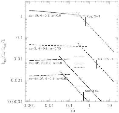
Figure 10: The ratio of the CS and bremsstrahlung luminosities (heavy and thin lines, respectively; the latter ratio is independent of $\dot{m}$) to the power dissipated in a patchy corona as functions of the accretion rate in the case of the coronal magnetic field strength equal to 0.5 of that inside the disc. The solutions corresponding to dominance of the gas pressure and radiation pressure are shown for $\dot{m}$ below and above $\sim\dot{m}_{\rm crit}$, respectively. The chosen values of $m$, $\Theta$, $\alpha$ are the same as in Figure 8. See Section 4.2.3 for details. The vertical bars mark our estimates of the accretion rates in 3 cases.

In the case of NGC 4258, we can reproduce the 2–10 keV power-law index and luminosity with $\Theta=0.43$ and $r_{\rm b}=2$. We note, however, that the CS luminosity is a sensitive function of the size of active regions in this model, $L_{\rm CS}\propto r_{\rm b}^{2}$ (which dependence is much stronger than that in the previous coronal models). Based on equation (39), we expect $r_{\rm b}$ decreasing with the decreasing $L$. If this is indeed the case for NGC 4258, the model of coronal CS emission could be then ruled out for this object (unless $\Theta>1$, as in the case discussed in Section 4.2.2 above).

We therefore again conclude that, in coronal models, the CS radiation can be important only in the case of stellar-mass sources with hard spectra. This radiative process is negligible in the case of objects with soft spectra (probably including low-luminosity sources) when Comptonization of photons from a cold accretion flow is expected to dominate. Note that if the disc magnetic field pressure is less than that of equipartition, e.g., by $\alpha_{\rm v}$ (Shakura & Sunyaev 1973), the predicted upper limits of $L_{\rm CS}$ would be even lower (e.g. by an order of magnitude for $\alpha_{\rm v}=0.1$).

We can compare our conclusions with those of Ghisellini, Haardt & Svensson (1998), who also consider magnetically dominated, patchy coronae and compare the relative importance of Comptonization of synchrotron and disc photons. They, however, do not assume a thermal electron distribution but instead assume a given form of electron acceleration and then calculate the electron distribution taking into account a balance between the acceleration, escape, Compton cooling and synchrotron emission and reabsorption. A resulting electron distribution consists typically of a quasi-thermal hump and a high-energy tail, which is an important difference with respect to the calculations presented here. Furthermore, they assume a constant magnetic field for a series of models with varying luminosity, and their magnetic field is not directly compared to that produced in the disc.

Still, their findings are compatible with ours. Namely, among the specific models they present, the CS process dominates only when $\Theta\sim 1$ and the magnetic energy density is more than one order of magnitude higher than that of radiation, see their Figure 4. We find that the parameters of their models with the CS process dominating, correspond approximately to $\eta\sim 10^{-4}$, i.e. to low-luminosity sources, in our model above (assuming $r_{\rm b}\sim 1$ and $N\sim 10$). Then, at $\Theta\sim 1$, we obtain predictions about the significance of the CS process similar to theirs.

5 Applications to accreting neutron stars

Power-law X-ray spectra are, in fact, observed not only from black-hole sources. Similar power laws are detected, e.g., from binary systems with weakly-magnetized neutron stars in the so-called low spectral state. Unambiguous classification of some of those sources as neutron stars comes from detections of type-1 X-ray bursts from them. Those spectra are often modelled by thermal Comptonization (e.g. Barret et al. 1999, hereafter B99), in which case the question arises of the origin of seed photons.

It is also of interest that accreting weakly-magnetized neutron stars show a number of similarities to accreting black holes (see e.g. a discussion in B99). First, this concerns timing properties in X-rays, namely time lags between soft and hard X-rays, which suggests similar geometries of the sources and/or similar variability mechanisms (e.g. Ford et al. 1999). Second, spectra of black holes in their hard states fit remarkably well a correlation between the 1–20 and 20–200 keV luminosities seen in neutron-star binaries (Barret, McClintock & Grindlay 1996) which may indicate that similar radiation mechanisms are operating in the two classes of objects. On the other hand, the presence of the neutron star results in more sources of soft photons than in the case of a black hole, namely thermal radiation from the surface of the star and synchrotron radiation in the stellar magnetic field.

Cyclotron radiation as a source of soft photons Comptonized in weakly magnetized accreting neutron stars has recently been considered by Psaltis (1998). In his model, self-absorbed cyclotron photons are produced in a layer above the stellar surface with $kT\sim 20$ keV and a magnetic field of $B\la 10^{10}$ G, and then subsequently Comptonized in a hot spherical corona of $kT\sim 10$ keV. Here, we consider a more generic geometry in which synchrotron photons are produced and Comptonized in the same medium, the temperature of which is determined from observations. This leads us to investigating plasmas of temperatures higher than those considered by Psaltis (1998). As in Section 4, we compare the luminosities in our model spectra to those observed.

We analyze here spectra of four X-ray bursters. The first one is 4U 0614+091, which low-state spectrum was fitted with the Comptonization model of Poutanen & Svensson (1996) by Piraino et al. (1999). They found the seed blackbody photons have $kT_{\rm BB}\la 30$ eV, and the plasma parameters are given by $\Theta\simeq 0.5$ and $\alpha=1.44$. The luminosity was $L_{\rm 1-200keV}\simeq 3.7\times 10^{36}$ erg s^-1 assuming $D=3$ kpc (Brandt et al. 1992). It is interesting that the above electron temperature is much higher than that seen from other X-ray bursters so far. The parameters of the second object in our sample, 1E 1724–3045, modeled by B99 with a Comptonization model of Titarchuk (1994) are $kT_{\rm BB}\simeq 1$ keV, $\Theta\simeq 0.057$, $\alpha=0.95$. (Since B99 did not give the spectral index of their fit, we have obtained it from the Comptonization model they used.) The luminosity, given $D=6.6$ kpc (Barbuy, Bica & Ortolani 1998), is $L_{\rm 1-200keV}\simeq 1.3\times 10^{36}$ erg s^-1. The third source is GS 1826–238, for which B99 found $\alpha=0.73$, and $\Theta\simeq 0.08$ from the high-energy tail with the model of Poutanen & Svensson (1996). At $D=7$ kpc (B99), $L_{\rm 1-200keV}\simeq 1.5\times 10^{36}$ erg s^-1. Observations of the fourth object, XB 1916–053, were reported by Church et al. (1998). The X-ray spectrum was fitted as a power-law of index $\alpha=0.61$ and the temperature was estimated from the cut-off in the spectrum to be $\Theta\simeq 0.06$. At $D=9$ kpc, $L_{\rm 0.5-200keV}\simeq 1.1\times 10^{36}$ erg s^-1 (Church et al. 1998).

We consider then a generic model with a spherical, uniform, plasma cloud, and investigate the relation between the size of the cloud and the magnetic field strength required to reproduce the observed luminosities at their spectral indices and temperatures. From equations (18) and (31), we expect that this relation will be roughly of the form of $B\propto R^{-0.7}$. We note that since a CS spectrum is normalized by its self-absorbed, optically-thick, part, the luminosity is roughly proportional to the source area, with the source geometry being only of secondary importance. Thus, our results may also approximate those for emission from a thin layer above the stellar surface. A second constraint on the model can be obtained from the fitted temperature of the seed photons, which is known for 4U 0614+091 and 1E 1724–3045. In those cases, we can identify the seed-photon temperature with the maximum possible turnover energy, $h\nu_{\rm t}\la kT_{\rm BB}$, which then yields an upper limit on $B$. This limit is $B\la 10^{8}$ G and $B\la 6\times 10^{9}$ G, respectively. In the case of GS 1826–238, the seed-photon temperature was not fitted, but we can estimate, from the shape of the spectrum presented by B99, that $kT_{\rm BB}\la 1$ keV, which yields $B\la 5\times 10^{9}$ G. We have no corresponding limit for XB 1916-053.

Figure 11: The relation between the size of the emission region and its magnetic field strength required for the CS process to reproduce the observed X-ray spectra and luminosities of four X-ray bursters (heavy lines). The thin horizontal lines show the upper limits on $B$ resulting from fitted constraints on the energy of seed photons. Both constraints have to be satisfied for the CS process to dominate.

The size–magnetic field relation obtained for the four objects is shown in Figure 11. Those results suggest that Comptonization may take place in a corona of the size comparable to the stellar radius ($\sim 10^{6}$ cm). The required magnetic field is then $B\la 10^{9}$ G. This value is consistent both with the upper limits resulting from fitting the energy of seed photons and with the maximum field strength possible in X-ray bursters, $B\la 10^{10}$–$10^{11}$ G, see Lewin, van Paradijs & Taam (1995). (Their constraint results from the requirement that the magnetic field does not funnel matter towards the magnetic poles, and more stringent constraints can be obtained for a specific structure of the accretion flow.)

We note that if Comptonization takes place close to the stellar surface, reflection albedo close to unity would be required. Otherwise reprocessing in the surface layers would result in a strong blackbody component, which is not seen.

We also find that it is unlikely that the size of the region where synchrotron photons (dominating the supply of seed photons) are produced and Comptonized is much larger than the neutron star radius. Such a configuration would be then similar to that of an optically thin disc around a black hole (Section 4.1) or an advection-dominated extended corona above a cold disc (Narayan, Barret & McClintock 1997). Then the required magnetic field, $B\sim 10^{8}$ G at $R\sim 10^{7}$ cm, would be too strong to be sustained by the disc [see equation (34), where we estimate the magnetic field in hot, optically thin, discs].

6 Discussion

A general feature of models of accretion flows around black holes considered above is the dependence of $B\propto m^{-1/2}$ [or very close to it, equation (46)]. This then implies decreasing values of $L_{\rm CS}/L_{\rm E}$ with $m$, and the relative importance of the CS process much weaker in AGNs than in black-hole binaries. The predicted values of $L_{\rm CS}$ strongly increase with increasing spectral hardness and temperature of the plasma. Compared with observations, we find that both the hot flow and coronal models can, in principle, explain emission of the hardest ($\alpha\sim 0.5$) among luminous (Eddington ratios of $\sim 0.01$), stellar-mass, sources in terms of the CS process. However, this process provides a negligible contribution to the luminosity, $L$, of luminous stellar-mass sources with soft spectra and of luminous AGNs regardless of $\alpha$. Taking into account the overall similarity between properties of luminous sources with either hard or soft spectra and containing either stellar-mass or supermassive black holes (e.g., Zdziarski 1999), it is likely that the CS process is in general energetically negligible in luminous sources.

However, the hot flow and coronal models differ in their predictions for the relative importance of the CS process with decreasing $L/L_{\rm E}$. In the hot flow model, there is clearly a range of $L/L_{\rm E}\ll 0.01$, in which the CS process can yield a dominant contribution to $L$ even in the case of AGNs. On the other hand, the coronal models have rather weak dependences of $L_{\rm CS}/L$ on $L/L_{\rm E}$. However, at some low value of $L/L_{\rm E}$, bremsstrahlung emission becomes dominant. Therefore, we have found that, in the coronal models, there is no range of $L/L_{\rm E}$ (except for hard, stellar-mass, sources, see above) in which the CS process could dominate energetically. In both models, bremsstrahlung is expected to give the main contribution to $L$ in very weak sources.

There are three complications in the picture above. First, the plasma parameters are expected, in general, to depend on $L/L_{\rm E}$, which will modify theoretical dependences of $L_{\rm CS}/L$ on the Eddington ratio. This is especially the case of the electron temperature, which is expected to be higher in low-luminosity sources, due to less efficient plasma cooling. This would strongly increase the efficiency of the CS process. We did not consider temperatures much higher than those observed in luminous objects, thus our conclusions about the role of the CS process in low-luminosity sources are rather conservative. Unfortunately, we have as yet no observational constraints on the plasma temperature in such sources.

Second, we have considered here accretion onto non-rotating black holes. Black-hole rotation increases, in general, the efficiency of accretion, and the CS process may yield then luminosities higher than those found here. This is, in fact, confirmed by a study of Kurpiewski & Jaroszyński (1999), who have considered advection-dominated flows and have found that an increase of the black-hole angular momentum leads to increase of the CS emission. This happens due to both the synchrotron emission itself as well its Comptonization becoming much more effective in innermost regions of the disc. Analysis of those issues is, however, beyond the scope of this work. Third, even when other processes dominate energetically, there can be a range of photon energies in which the CS process gives the dominant contribution.

Still, the strong conclusion of Section 4 is that the thermal CS process does not dominate observed X-ray spectra of luminous black-hole sources. Rather, the dominant X-ray producing process in those sources appears to be Comptonization of blackbody photons emitted by some optically-thick medium, e.g., an optically-thick accretion disc or clumps of cold matter. Observationally, the presence of such component is indicated by the wide-spread presence of Compton reflection from a cold medium in luminous black-hole sources (e.g. Zdziarski et al. 1999) as well as observations of blackbody-like soft X-ray components in spectra of black-hole binaries (e.g. Ebisawa et al. 1994). Furthermore, a very strong correlation between the reflection strength and the X-ray spectral index is present in those sources (Zdziarski et al. 1999), in particular in Cyg X-1 and GX 339–4 (Gilfanov, Churazov & Revnivtsev 1999; Revnivtsev, Gilfanov & Churazov 1999). The presence of such correlation is naturally explained in models with plasma cooling due to blackbody emission of cold matter, whereas it cannot be explained if the CS process dominates.

On the other hand, we find in Section 5 that the thermal CS process can easily account for power law emission of weakly magnetized neutron stars in their low states. A possible caveat for that model is that a correlation between reflection and $\alpha$ has been observed in 4U 0614+091 (Piraino et al. 1999), although its interpretation remains ambiguous due to the lack of a detection of blackbody emission strong enough to provide seed photons for Comptonization.

We point out that a small non-thermal tail in the electron distribution due to acceleration (as in the model of Ghisellini et al. 1998), e.g. stochastic or in reconnection events could significantly increase the turnover frequency (since electrons with $\gamma\gg 1$ are usually responsible for emission at the turnover frequency), and thus increase the CS luminosity from accreting black holes and neutron stars. This issue is the subject of our work in progress.

Finally, we notice thermal Comptonization may be (at most) a secondary process in spectral formation in some classes of compact X-ray sources. One important class of such sources are black-hole binaries in the soft state, which X-ray and soft $\gamma$-ray spectra appear non-thermal (e.g. Gierliński et al. 1999). In that case, the X-ray spectrum contains a very strong blackbody component, which probably dominates over synchrotron photons as seeds for non-thermal Comptonization.

7 Conclusions

The main results of this work can be outlined as follows.

We have derived and tested analytic approximations for the synchrotron emission coefficient in thermal plasmas, applicable especially to the semi-relativistic range of temperatures, $T\sim 10^{9}$ K. We have also obtained analytic approximations to the turnover frequency (at which the plasma becomes optically-thick to absorption).

Then, we have presented a method to treat thermal Comptonization of synchrotron radiation. Our approximate analytic expressions allow for self-consistent calculations of the spectrum and the luminosity of such a source and can be easily applied to models of accretion discs.

We have also investigated the role of the thermal CS process in accretion flows around stellar-mass and supermassive black holes. We have considered two main scenarios: a hot, two-temperature, optically-thin flow and active regions above a cold, optically-thick disc. We have found that this process is only marginally important in luminous X-ray sources containing accreting black holes, and it can possibly dominate only in stellar-mass sources with hardest spectra. The dominant radiative process in those sources appears to be Comptonization of blackbody radiation emitted by cold matter in the vicinity of the hot plasma. On the other hand, the CS process can explain X-ray spectra of weaker sources, e.g., low-luminosity AGNs, but only in the hot-flow model. Finally, below certain low luminosity, bremsstrahlung becomes the dominant process.

Finally, we considered the case of weakly-magnetized accreting neutron stars. We have found that their power-law X-ray spectra in the low state can be accounted for by the CS process taking place in a corona of the size comparable to the stellar radius.

References

- [] Abramowicz M. A., Chen X., Kato S., Lasota J.-P., Regev O., 1995, ApJ, 438, L37
- [] Abramowitz M., Stegun I. A., 1970, Handbook of Mathematical Functions. Wiley, New York (AS70)
- [] Balbus S. A., Hawley J. F., 1998, Rev. Mod. Phys., 70, 1
- [] Barbuy B., Bica E., Ortolani S., 1998, A&A, 333, 117
- [] Barret D., McClintock J. E., Grindlay J. E., 1996, ApJ, 303, 526
- [] Barret D., Olive J. F., Boirin L., Done C., Skinner G. K., Grindlay J. E., 1999, ApJ, in press (B99)
- [] Bekefi G., 1966, Radiation Processes in Plasmas. Wiley, New York
- [] Beloborodov A. M., 1999, ApJ, 510, L123
- [] Brandt S., Castro-Tirado A. J., Lund N., Dremin V., Lapshov I., Sunyaev R., 1992, A&A, 262, L15
- [] Chanmugam G, Barrett P. E., Wu K., Courtney M. W., 1989, ApJS, 71, 323
- [] Chen X., Abramowicz M. A., Lasota J. P., 1997, ApJ, 476, 61
- [] Church M. J., Parmar A. N., Bałucińska-Church M., Oosterbrock T., Dal Fiume D., Orlandini M., 1998, A&A, 338, 556
- [] Clavel J., et al., 1987, ApJ, 321, 251
- [] Dermer C. D., Liang E. P, Canfield E., 1991, ApJ, 369, 410
- [] Di Matteo T., 1998, MNRAS, 299, L15
- [] Di Matteo T., Blackman E. G., Fabian A. C., 1997a, MNRAS, 291, L23
- [] Di Matteo T., Celotti A., Fabian A. C., 1997b, MNRAS, 291, 805 (DCF97)
- [] Di Matteo T., Celotti A., Fabian A. C., 1999, MNRAS, 304, 809
- [] Dulk G. A., 1985, ARA&A, 23, 169
- [] Ebisawa K., Ueda Y., Inoue H., Tanaka Y., White N. E., 1996, ApJ, 467, 419
- [] Eckart A., Genzel R., 1996, Nat, 383, 415
- [] Ford E. C., van der Klis M., Méndez M., van Paradijs J., Kaaret P., 1999, ApJ, 512, L31
- [] Galeev A. A., Rosner R., Vaiana G. S., 1979, ApJ, 229, 318
- [] Ghisellini G., Haardt F., Svensson R., 1998, MNRAS, 297, 348
- [] Gierliński M., Zdziarski A. A, Done C., Johnson W. N., Ebisawa K., Ueda Y., Haardt F., Phlips B. F., 1997, MNRAS, 288, 958
- [] Gierliński M., Zdziarski A. A, Poutanen J., Coppi P. S., Ebisawa K., Johnson W. N., 1999, MNRAS, 309, 496
- [] Gilfanov M., Churazov E., Revnivtsev M., 1999, A&A, in press
- [] Hartmann D., Woosley S. E., Arons J., 1988, ApJ, 332, 777
- [] Hawley J. F., Gammie C. F., Balbus S. A., 1995, ApJ, 440, 742
- [] Jones, T. W., Hardee, P. E., 1979, ApJ, 228, 268
- [] Kurpiewski A., Jaroszyński M., 1999, A&A, 346, 713
- [] Lasota J.-P., Abramowicz M. A., Chen X., Krolik J., Narayan R., Yi I., 1996, ApJ, 462, 142
- [] Lewin W. H. G., van Paradijs J., Taam R. E., 1995, in Lewin W. H. G., van den Heuvel E. P. J., van Paradijs J., eds., X-ray Binaries, Cambridge Univ. Press, Cambridge, p. 175
- [] Lightman A. P., Zdziarski A. A., 1987, ApJ, 319, 643
- [] Longair M. S., 1992, High Energy Astrophysics. Cambridge University Press, Cambridge
- [] Mahadevan R., 1997, ApJ, 477, 585
- [] Mahadevan R., Narayan R., Yi I., 1996, ApJ, 465, 327 (MNY96)
- [] Makishima K. at al., 1994, PASJ, 46, L77
- [] Malysheva L. K., 1997, Astron. Lett., 23, 585 [in Russian: AZh Pisma, 23, 667]
- [] Massey P., Johnson K. E., DeGioia-Eastwood K., 1995, ApJ, 454, 171
- [] Miyamoto S., Kitamoto S., Sayuri I., Negoro H., Terada K., 1992, ApJ, 391, L21
- [] Miyoshi M. et al., 1995, Nat, 373, 127
- [] Narayan R., Yi I., 1995, ApJ, 452, 710 (NY95)
- [] Narayan R., Barret D., McClintock J. E., 1997, ApJ, 482, 448
- [] Narayan R., Mahadevan R., Grindlay J. E., Popham R. G., Gammie C., 1998, ApJ, 492, 554
- [] Osterbrock D. E., 1974, Astrophysics of Gaseous Nebulae. Freeman, San Francisco
- [] Pacholczyk A. G., 1970, Radio Astrophysics. Freeman, San Francisco
- [] Peterson B. M., 1997, Active Galactic Nuclei. Cambridge University Press, Cambridge
- [] Petrosian V., 1981, ApJ, 251, 727 (P81)
- [] Petrosian V., McTiernan J. M., 1983, Phys. Fluids, 26, 3023
- [] Piraino S., Santangelo A., Ford E. C., Kaaret P., 1999, A&A, 349, L77
- [] Poutanen J., Svensson R., 1996, ApJ, 470, 249
- [] Psaltis D., 1998, PhD Thesis, University of Illinois
- [] Revnivtsev M., Gilfanov M., Churazov E., 1999, A&A, in press
- [] Robinson P. A., Melrose D. B., 1984, Australian J. Phys., 37, 675
- [] Rybicki G. R., Lightman A. P., 1979, Radiative Processes in Astrophysics. Wiley-Interscience, New York
- [] Scheuer P. A. G., 1968, ApJ, 151, L139
- [] Shakura N. I., Sunyaev R. A., 1973, A&A, 24, 337
- [] Shapiro S. L., Lightman A. P., Eardley D. M., 1976, ApJ, 204, 187
- [] Sunyaev R. A., Titarchuk L. G., 1980, A&A, 86, 121
- [] Svensson R., 1984, MNRAS, 209, 175
- [] Svensson R., Zdziarski A. A., 1994, ApJ, 436, 599
- [] Takahara F., Tsuruta S., 1982, Prog. Theor. Phys., 67, 485
- [] Titarchuk L., 1994, ApJ, 434, 313
- [] Trubnikov B. A., 1958, Doklady Akad. Nauk. SSSR, 118, 913
- [] Wind J. P., Hill E. R., 1971, Australian J. Phys., 24, 43
- [] Zdziarski A. A., 1985, ApJ, 289, 514 (Z85)
- [] Zdziarski A. A., 1986, ApJ, 303, 94 (Z86)
- [] Zdziarski A. A., 1999, in Poutanen J., Svensson R., eds., High Energy Processes in Accreting Black Holes, ASP Conf. Series 161, p. 16
- [] Zdziarski A. A., Fabian A. C., Nandra K., Celotti A., Rees M. J., Done C., Coppi P. S., Madejski G. M., 1994, MNRAS, 269, L55
- [] Zdziarski A. A., Johnson W. N., Magdziarz P., 1996, MNRAS, 283, 193
- [] Zdziarski A. A., Poutanen J., Mikołajewska J., Gierliński M., Ebisawa K., Johnson W. N., 1998, MNRAS, 301, 435
- [] Zdziarski A. A., Lubiński P., Smith D. A., 1999, MNRAS, 303, L11