Spherical Infall Model in a Cosmological Background Density Field

Abstract

We discuss the influence of the cosmological background density field on the spherical infall model. The spherical infall model has been used in the Press-Schechter formalism to evaluate the number abundance of clusters of galaxies, as well as to determine the density parameter of the universe from the infalling flow. Therefore, the understanding of collapse dynamics play a key role for extracting the cosmological information. Here, we consider the modified version of the spherical infall model. We derive the mean field equations from the Newtonian fluid equations, in which the influence of cosmological background inhomogeneity is incorporated into the averaged quantities as the backreaction. By calculating the averaged quantities explicitly, we obtain the simple expressions and find that in case of the scale-free power spectrum, the density fluctuations with the negative spectral index make the infalling velocities slow. This suggests that we underestimate the density parameter $\Omega$ when using the simple spherical infall model. In cases with the index $n>0$, the effect of background inhomogeneity could be negligible and the spherical infall model becomes the good approximation for the infalling flows. We also present a realistic example with the cold dark matter power spectrum. There, the anisotropic random velocity leads to slowing down the mean infalling velocities.

1 Introduction

In the standard scenario of the cosmic structure formation, the density peaks in the large-scale inhomogeneities grow due to the gravitational instability and they experience the gravitational collapse, which finally lead to the virialized objects such as the clusters of galaxies or the dark matter halos.

Modeling such non-linear objects plays an important role for probing the large scale structure. After the seminal paper by Gunn & Gott (1972), the spherical infall model has been extensively used in the literature. The non-linear system mimicking the density peak is represented by the spherical overdensity with the radius $R$, which obeys the simple dynamics (Peebles 1980)

$$\ddot{R}+\frac{GM}{R^{2}}=0,$$ (1)

where $M$ is the mass of the bound object. The density contrast of this non-linear object is defined by $\delta=(a/R)^{3}-1$, where $a$ is the expansion factor of the universe. From (1), we can estimate the collapse time $t_{c}$, which gives the dynamical time scale of the virialization. In terms of the linearly extrapolated density contrast, we have the value $\delta_{c}\equiv\delta(t_{c})\simeq 1.68$ in the Einstein-de Sitter universe (for the low density universe or the flat universe with the non-vanishing cosmological constant, see e.g, Eke, Coles & Frenk 1996). This is frequently used in the Press-Schechter mass function to evaluate the number abundance of cluster of galaxies (Press & Schechter 1974, Eke, Coles & Frenk 1996, Kitayama & Suto 1997).

Further, the spherical infall model can also be applied to estimate the density parameter of our universe, although the other efficient method such as POTENT has recently been available (e.g, Bertschinger & Dekel 1989, see also the review by Strauss & Willick 1995). The observation of the infalling velocity $V_{\rm inf}$ can be compared to the expansion rate $\dot{R}/R$ subtracting the uniform Hubble flows. Characterizing the infalling velocity $V_{\rm inf}$ as the function of mean overdensity $\bar{\delta}$ within the sphere centered on the core of cluster, we can determine $\Omega$ from the $\bar{\delta}$-$V_{\rm inf}$ relation (Davis & Huchra 1982, Yahil 1985, Dressler 1988).

As we know, the spherical infall model is the ideal system. In real universe, the density peak cannot evolve locally. The cosmological background density field affects the dynamical evolution and the collapsed time of the density peak. This might lead to the incorrect prediction for the low mass objects using the Press-Schechter formalism (Jing 1998, Sheth, Mo & Tormen 1999). As for the infall velocity, the tidal effect distorts the flow field around the core of cluster, which becomes the source of the underestimation of the density parameter (Villumsen & Davis 1986).

Therefore, the understanding of the influence of cosmological background density field on the bound objects is crucial to clarify the cosmic structure formation. Several authors treat this issue and consider the modification of the spherical infall model taking into account the background density inhomogeneity (Hoffman 1986, Bernardeau 1994, Eisenstein & Loeb 1995). The validity of the spherical infall model and the estimation of the collapsed time scale have been mainly discussed. Another author evaluates the weakly non-linear correction of the background density field using the conditional probability distribution function around the overdensity and studies the influence of the non-linear density inhomogeneities to the dark matter density profiles (Łokas 1998).

In this paper, we investigate the influences of the cosmic background density field on the spherical infall model using the different approach from the previous works. Focusing on the mean expansion around the bound system, the Gauss’ law implies that the interior of the bound object can be regarded as the homogeneous overdensity by taking the averaging procedure. Hence, we will treat the averaged dynamics of the inhomogeneous gravitational collapse. The influence of cosmic density fields on the infalling velocity is incorporated into the averaged quantities as the backreaction of the growing inhomogeneities. Importantly, the modified dynamics can be non-local. In addition to the mass $M$ of the bound object, the evolution depends on the statistical property of the density fluctuations.

In section 2, we first argue how the background density field modifies the non-linear dynamics (1). Then, we derive the evolution equations for overdensity by averaging the inhomogeneous Newtonian gravity. The modified dynamics can contain the averaged quantities characterizing the backreaction of the cosmic density inhomogeneity. We explicitly calculate these quantities in the Appendix A and obtain the simple expressions. The main results in this paper are equations (20) and (21). Using these expressions, we further discuss the influence of backreaction effect on the infalling velocity in section 3. Final section 4 is devoted to the summary and discussions.

2 Averaged dynamics of spherical infall model

2.1 The backreaction of cosmic density field

We shall start with the basic equations for Newtonian dust fluid:

$$\frac{\partial\rho}{\partial\tau}+\vec{\nabla}_{X}(\rho\vec{v})=0,$$

$$\frac{\partial\vec{v}}{\partial\tau}+(\vec{v}\cdot\vec{\nabla}_{X})\vec{v}=-\vec{\nabla}_{X}\phi$$ (2)

$$\nabla_{X}^{2}\phi=4\pi G\rho,$$

where $\tau$ is the proper time of the dust fluid and $\vec{\nabla}_{X}$ is the derivative with respect to the proper distance $\vec{X}$ from some chosen origin.

The non-linear dynamics of spherical overdensity (1) is embedded in the above system. Consider the homogeneous infalling flow, in which the quantities $\rho$, $\vec{v}$ and $\phi$ are given by

$$\rho = \bar{\rho}(\tau)$$

$$\vec{v} = {\cal H}(\tau)\vec{X}~{};~{}~{}~{}~{}~{}{\cal H}=\frac{\dot{R}}{R},$$

$$\phi = \frac{2}{3}\pi G~{}\bar{\rho}(\tau)~{}|\vec{X}|^{2}$$

where $R$ is the proper radius of the spherical overdensity. We then introduce the comoving frame $(t,\vec{x})$ defined as

$$\tau=t,~{}~{}~{}~{}~{}~{}~{}\vec{X}=R(t)\vec{x}.$$ (3)

Substitution of (2.1) into (2) yields

$$\dot{\bar{\rho}}+3{\cal H}\bar{\rho}=0,~{}~{}~{}~{}~{}3\dot{\cal H}+3{\cal H}+4\pi G\bar{\rho}=0,$$ (4)

where $(\dot{~{}})$ denotes the derivative with respect to the time $t$. Because the first equation implies the mass conservation $M=(4\pi/3)\bar{\rho}R^{3}$, the homogeneous system (4) is equivalent to the dynamics (1).

When we take into account the cosmic background density field, the dynamics of overdensity affects the evolution of background inhomogeneity and the growth of inhomogeneities induces the tidal force, which distorts the homogeneous evolution of the infalling flows. The situation we now investigate is that the background fluctuation is not so large and the dynamics of overdensity is dominated by the radial motion, that is, the dynamics could be almost the spherically symmetric collapse. In this case, we can approximately treat the radial infalling flows as the homogeneous system and the evolution of the overdensity is solely affected by the small perturbation of the background density fields.

Therefore, the problem is reduced to a classic issue of the backreaction. That is, together with the quantities $(\bar{\rho},{\cal H})$, the dynamics of the homogeneous overdensity can be determined by the backreaction of background inhomogeneities through the non-linear interaction. Phenomenologically, the backreaction effect can be mimicked by adding the non-vanishing terms characterizing the density inhomogeneity in the right hand side of equations (4). Here, we consider the self-consistent treatment based on the equations (2). We will derive the dynamics of infalling flows including the backreaction effect. Since the evolution of overdensity is affected by the spatial randomness of the cosmic inhomogeneity, it should be better to investigate the mean dynamics of the overdensity, which can be derived from the system (2) taking the spatial averaging.

Let us divide the quantities $\rho$, $\vec{v}$ and $\phi$ into the homogeneous part and the fluctuating part with the zero mean:

$$\rho = \bar{\rho}(\tau)+\delta\rho(\tau,\vec{X}),$$

$$\vec{v} = {\cal H}(\tau)\vec{X}+\vec{u}(\tau,\vec{X}),$$ (5)

$$\phi = \frac{2}{3}\pi G~{}\bar{\rho}(\tau)~{}|\vec{X}|^{2}+\Phi(\tau,\vec{X}).$$

Substituting (5) into (2), the equation of continuity becomes

$$\left(\dot{\bar{\rho}}+3{\cal H}\bar{\rho}\right)+\left(\frac{\partial\delta\rho}{\partial t}+3{\cal H}\delta\rho+\frac{\bar{\rho}}{R}\vec{\nabla}_{x}\vec{u}\right)$$

$$~{}~{}~{}~{}~{}~{}~{}~{}~{}~{}~{}~{}~{}~{}~{}~{}~{}~{}~{}~{}~{}~{}~{}~{}~{}~{}~{}~{}~{}~{}~{}~{}~{}~{}~{}~{}~{}~{}~{}~{}=-\frac{1}{R}\vec{\nabla}_{x}(\delta\rho~{}\vec{u}).$$ (6)

For the Euler equation, taking the spatial divergence yields

$$\left(3\dot{\cal{H}}+3{\cal H}^{2}+4\pi G\bar{\rho}\right)+\frac{1}{R}\vec{\nabla}_{x}\left(\frac{\partial\vec{u}}{\partial t}+{\cal H}\vec{u}+\frac{1}{R}\vec{\nabla}_{x}\Phi\right)$$

$$~{}~{}~{}~{}~{}~{}~{}~{}~{}~{}~{}~{}~{}~{}~{}~{}~{}~{}~{}~{}~{}~{}~{}~{}~{}~{}~{}~{}~{}~{}=~{}-\frac{1}{R^{2}}\nabla_{x}\left[(\vec{u}\cdot\vec{\nabla}_{x})\vec{u}\right].$$ (7)

In equations (6) and (7), the non-linear interaction of the background inhomogeneities are expressed in the right hand side of these equations.

The system (6) and (7) can be divided into the homogeneous part and the fluctuating part by taking the spatial average over the comoving volume $V_{r}=(4\pi/3)r_{0}^{3}$, where the radius $r_{0}$ denotes the comoving size of the characteristic overdensity. The spatial averaging is defined as

$$\langle\langle\cdots\rangle\rangle=\frac{1}{V_{r}}\int_{V_{r}}d^{3}x~{}\langle\cdots\rangle,$$ (8)

where $\langle\cdots\rangle$ denotes the ensemble average taken over the random fluctuations $\delta\rho$ and $\vec{u}$. Then, we obtain

$$\dot{\bar{\rho}}+3{\cal H}\bar{\rho}=-\frac{1}{R}\langle\langle\vec{\nabla}_{x}\left[\delta\rho~{}\vec{u}\right]\rangle\rangle,$$ (9)

$$\frac{\ddot{R}}{R}+\frac{4\pi G}{3}\bar{\rho}=-\frac{1}{3R^{2}}\langle\langle\vec{\nabla}_{x}\left[(\vec{u}\cdot\vec{\nabla}_{x})\vec{u}\right]\rangle\rangle$$ (10)

for the homogeneous part and

$$\frac{\partial\delta\rho}{\partial t}+3{\cal H}\delta\rho+\frac{1}{R}\vec{\nabla}_{x}\vec{u}=0,$$

$$\frac{\partial\vec{u}}{\partial t}+{\cal H}\vec{u}=\frac{1}{R}\vec{\nabla}_{x}\Phi=0,$$ (11)

$$\nabla_{x}^{2}\Phi=4\pi GR^{2}\delta\rho,$$

for the fluctuating part with the zero mean.

The results (9), (10) and (11) are the desirable forms for our purpose. The mean dynamics of overdensity is affected by the the averaged quantities $\langle\langle\cdots\rangle\rangle$ corresponding to the backreaction of the cosmic density inhomogeneities. These quantities are evaluated self-consistently by solving the evolution equations (11) under the knowledge of homogeneous quantities $\bar{\rho}$ and $R$.

2.2 The averaged quantities

We proceed to analyze the mean dynamics (9) and (10). In general relativity, the quantitative analysis of the backreaction terms is still hampered by a more delicate issue of the gauge conditions even after deriving the basic equations (Buchert 1999). However, in the Newton gravity, we are not worried about the evaluation of the averaged quantities. Let us separate the variables $\delta\rho$, $\vec{u}$ and $\Phi$ into the the time-dependent part and the spatial random part:

$$\delta\rho = ~{}D(t)~{}\hat{\delta}(x),$$

$$\vec{u} = ~{}G~{}R(t)V(t)~{}\vec{\nabla}_{x}\hat{\Delta}(x),$$ (12)

$$\Phi = ~{}G~{}R^{2}(t)D(t)~{}\hat{\Delta}(x),$$

where the variables with $(\hat{~{}})$ denote the random field. The ensemble average is taken with respect to these variables. Then, the evolution equations (9), (10) and (11) become the four set of ordinary differential equation:

$$\dot{\bar{\rho}}~{}~{}+~{}~{}3{\cal H}\bar{\rho} = -G(DV)~{}{\bf C}_{1},$$ (13)

$$\frac{\ddot{R}}{R}~{}+\frac{4\pi G}{3}\bar{\rho} = -\frac{G^{2}}{3}V^{2}~{}{\bf C}_{2},$$ (14)

$$\dot{D}~{}+~{}3{\cal H}D = 4\pi G~{}\bar{\rho}~{}V,$$ (15)

$$\dot{V}~{}+~{}2{\cal H}V = D,$$ (16)

where

$${\bf C}_{1} = \frac{\langle\langle\vec{\nabla}_{x}\left[\delta\rho~{}\vec{u}~{}\right]\rangle\rangle}{G~{}(RVD)},$$

$${\bf C}_{2} = \frac{\langle\langle\vec{\nabla}_{x}\left[(\vec{u}\cdot\vec{\nabla}_{x})\vec{u}\right]\rangle\rangle}{G^{2}(RV)^{2}}$$

are merely the numerical constants. Provided the statistical feature of the spatial inhomogeneities $\hat{\delta}$ and $\hat{\Delta}$, we can evaluate ${\bf C}_{1}$ and ${\bf C}_{2}$. Notice that both $\hat{\delta}$ and $\hat{\Delta}$ are related through the Poisson equation:

$$\nabla^{2}_{x}~{}\hat{\Delta}=~{}-4\pi~{}\hat{\delta}.$$ (17)

Thus, the non-local tidal effect induced by the cosmic density fields can be treated in our prescription.

To evaluate the averaged quantities ${\bf C}_{1},~{}{\bf C}_{2}$, it is sufficient to know the second order statistics of the density inhomogeneities, i.e, the power spectrum $P(k)$. Usually, $P(k)$ is given by

$$\langle\hat{\delta}(\vec{k})\hat{\delta}(\vec{k}^{\prime})\rangle=(2\pi)^{3}\delta_{D}(\vec{k}+\vec{k}^{\prime})~{}P(k)$$ (18)

in the Fourier representation. However, the naive computation using the above definition gives the monopole term, i.e, $l=0$ mode of the spherical harmonic expansion for the fluctuations. In our approach, the coherent radial motion arising from the monopole contribution has already been renormalized in the homogeneous system, that is, the fluctuations defined in (5) have only the higher multipole $l\geq 1$. This means that the alternative definition subtracting the monopole term

$$\langle\hat{\delta}(\vec{k})\hat{\delta}(\vec{k}^{\prime})\rangle=(2\pi)^{3}~{}P(k)\left[\delta_{D}(\vec{k}+\vec{k}^{\prime})-\frac{1}{4\pi k^{2}}\delta_{D}(k-k^{\prime})\right]$$ (19)

should be used in our formalism.

The calculation using (19) is essential to obtain the non-vanishing averaged quantities. In the Appendix A, the details of calculation for averaged quantities are described. Here, we present the final expressions:

$${\bf C}_{1} = \frac{8}{V_{r}}\left\{\xi_{0}(r_{0})-\xi_{1}(r_{0})\right\}.$$ (20)

$${\bf C}_{2} = \frac{32\pi}{3~{}V_{r}}\left\{-\xi_{0}(r_{0})+3\xi_{1}(r_{0})-2\xi_{2}(r_{0})\right\},$$ (21)

The function $\xi_{l}(r_{0})$ denotes the statistical quantity given by

$$\xi_{l}(r_{0})\equiv~{}\int_{0}^{r_{0}}dr~{}\int_{0}^{\infty}dk~{}(kr)^{2}~{}P(k)\left[j_{l}(kr)\right]^{2},$$ (22)

where $j_{l}(x)$ is the spherical Bessel function for $l$-th order.

Equations (20) and (21) are the main results of this paper. From these expressions, we immediately see that the backreaction effect becomes negligible on large scales due to the suppression factor $1/V_{r}$. This is correct in the cases with the power-law spectrum $P(k)\propto k^{n}$ within the range $-3<n<1$. In the limit $r_{0}\to\infty$, the dynamics (9) and (10) can be well-approximated by the spherical infall model (1).

Figure 1: The averaging quantities ${\bf C}_{1,2}$ as the function of $n$ for a power-law spectrum $P(k)~{}\propto~{}k^{n}.$ The thin and thick lines respectively denote the quantities ${\bf C}_{1}$ and ${\bf C}_{2}$, which are evaluated from (20) and (21) using the expressions (24) and (25).

Figure 2: The ratio of the infalling velocity to the Hubble flow as the function of the spectral index $n$ (long-dashed, short-dashed, dotted, dot-dashed-lines). By solving the mean dynamics (13)-(16), the quantity given by (28) is evaluated at the time $a_{f}/a_{i}=4$ in the Einstein-de Sitter universe. We choose the initial density contrast $\bar{\delta}=0.3$. The initial condition for the fluctuating part are described by the linear growing mode of perturbations neglecting the backreaction effect. The results are compared to the homogeneous infalling flow obtained from the simple dynamics (1)(thin-solid line).

3 Effects on the infalling velocity

Provided the power spectrum $P(k)$ of the background density fluctuations, we can investigate the mean infalling flows around the density peak. For the present purpose, it is useful to consider the scale-free spectrum in more detail:

$$P(k)=A~{}k^{n}.$$ (23)

Then the quantity $\xi_{l}(r_{0})$ can be expressed in terms of the gamma functions. We have

$$\xi_{l}(r_{0})=-A~{}r_{0}^{-n}~{}\frac{2^{n}\pi}{n}~{}\frac{\Gamma{(-n-1)}\Gamma{(l+(3+n)/2)}}{[\Gamma{(-n/2)}]^{2}\Gamma{(l+(1-n)/2)}}.$$ (24)

The power spectrum is related to the variance of density fluctuations $\sigma_{\scriptscriptstyle\rm TH}$, where the subscript _TH means the variable with the top-hat smoothing. Identifying the smoothing radius with the comoving radius of overdensity $r_{0}$, the influence of the background inhomogeneities to the overdensity can be quantified by $\sigma_{\scriptscriptstyle\rm TH}$. Then, the normalization factor $A$ is given by

$$A=\frac{4\pi}{3}~{}r_{0}^{3+n}\sigma_{\scriptscriptstyle\rm TH}^{2}~{}\frac{[\Gamma((2-n)/2)]^{2}\Gamma((3-n)/2)}{2^{n-1}\Gamma(1-n)\Gamma((3+n)/2)}.$$ (25)

Thus, the averaged quantities can be characterized by the three parameters, $r_{0}$, $n$ and $\sigma_{\scriptscriptstyle\rm TH}$.

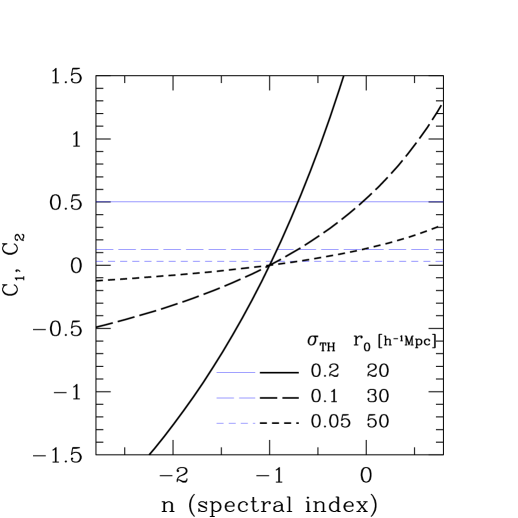
In Fig.1, we plot the averaged quantities as the function of the spectral index $n$. The typical parameters are respectively chosen as follows: $\sigma_{\scriptscriptstyle\rm TH}=0.2$ and $r_{0}=20~{}h^{-1}$ Mpc (solid line); $\sigma_{\scriptscriptstyle\rm TH}=0.1$ and $r_{0}=30~{}h^{-1}$ Mpc (long-dashed line) ; $\sigma_{\scriptscriptstyle\rm TH}=0.05$ and $r_{0}=50~{}h^{-1}$ Mpc (short-dashed line). Fig.1 says that as the variance $\sigma_{\scriptscriptstyle\rm TH}$ decreases and/or the radius $r_{0}$ increases, the quantities ${\bf C}_{1}$ and ${\bf C}_{2}$ become negligible. The thick lines shows the variable ${\bf C}_{2}$. Interestingly, ${\bf C}_{2}$ turns its signature. The negative value is obtained at $n<-1$, while we have the positive value ${\bf C}_{2}$ at $n>-1$. By contrast, the quantity ${\bf C}_{1}$ denoted as the thin lines becomes positive and almost constant over the range $-2.8<n<0.8$.

Fig.1 indicates that backreaction of the cosmic density inhomogeneities can prevent the spherical shell from infalling into the center of overdensity for the negative spectral index (see eqs.[13][14]). The effect becomes noticeable when $n<-1$. The result can be interpreted as follows. The quantities ${\bf C}_{2}$ is expressed in terms of the geometrical optics. From (12), we can write the peculiar velocity as $\partial_{i}u_{j}=(\theta/3)\delta_{ij}+\sigma_{ij}$, where $\theta$ and $\sigma_{ij}$ are the expansion scalar and the shear tensor, respectively. Then we have

$$\langle\langle\vec{\nabla}_{x}\left[(\vec{u}\cdot\vec{\nabla}_{x})\vec{u}\right]\rangle\rangle=\langle\langle\frac{1}{3}\theta^{2}\rangle\rangle+\langle\langle\sigma_{ij}\sigma^{ij}\rangle\rangle+\langle\langle\vec{u}\cdot\vec{\nabla}\theta\rangle\rangle.$$ (26)

The last term in the right-hand side of (26) means the flows of inertial frame. It is easy to show that the first and the second terms in the right-hand side of (26) always become positive. On the other hand, the last term can be written by

$$\frac{\langle\langle\vec{u}\cdot\vec{\nabla}\theta\rangle\rangle}{G^{2}(RV)^{2}}=-\frac{32\pi}{V_{r}}\left[\sum_{l=0}(2l+1)\xi_{l}(r_{0})-\xi_{1}(r_{0})\right],$$ (27)

which is always negative. This means that the anisotropic flows of cosmic density field can induce the effective pressure and this could dominate the expansion and the shear terms. The effect becomes significant when the long wavelength fluctuations have the large power, corresponding to the small spectral index $n<-1$. Accordingly, the background inhomogeneity apparently prevents the collapse of the averaged overdensity.

To see the backreaction effect more explicitly, we analyze the infalling velocity. The flow field around the spherical overdensity can be quantified by

$$\frac{V_{\rm inf}}{H|\vec{r}|}\equiv\frac{H-{\cal H}}{H}.$$ (28)

The above quantity can be evaluated by solving the evolution equations (13)-(16).

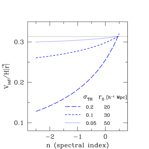
In Fig.2, we plot the ratio of the infalling velocity to the Hubble flow as the function of the spectral index. Here, the cosmic expansion is assumed to be that of the Einstein-de Sitter universe, $a=(t/t_{i})^{2/3}$. The initial velocity flow ${\cal H}$ of the overdensity is obtained by equating it with the Hubble expansion. As for the initial overdensity, $\bar{\rho}$ can be characterized by the density contrast $\bar{\delta}=\bar{\rho}/\rho_{b}-1$, where $\rho_{b}$ is the homogeneous density of the universe. We choose the initial density contrast as $\bar{\delta}=0.3$. On the other hand, the evolution of the fluctuating part $D$ and $V$ can be initially described by the linear growing mode neglecting the backreaction effect. Then, we solve the evolution equations by varying the spectral index $n$. The results are depicted when the final expansion factor $a_{f}$ becomes four times larger than the initial expansion factor $a_{i}$, i.e, $a_{f}/a_{i}=4$, within the validity of the approximation neglecting the higher order perturbations.

In Fig.2, we also plot the ratio $V_{\rm inf}/H|\vec{r}|$ evaluated from the spherical infall model (1) (thin-solid line). Clearly, the deviation from the spherical infall model becomes significant for the small radius of the overdensity and the large variance of the fluctuations (thick-long-dashed, thick-short-dashed lines). The cosmic background inhomogeneity can weaken the infalling velocity. This effect leads to the overestimation of the cosmic expansion when we compare the observation of the infalling velocity with the spherical infall model. Consequently, we would prefer the low density universe. However, the deviation becomes small as the spectral index increases. The backreaction effect becomes negligible and the infalling velocity can be well-described by the spherical infall model. At the time $a_{f}/a_{i}=4$, the index $n\approx 0.5$ is marginal, which is rather larger value than $n=-1$.

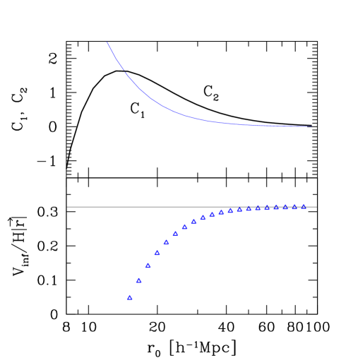
As another example, a realistic case with the cold dark matter (CDM) spectrum is examined. In Fig.3, we specifically consider the standard CDM, i.e, $\Omega_{0}=1$ and $\lambda_{0}=0$. The fitting form of the power spectrum given by Bardeen et al. (1986) is used and normalized by the top-hat fluctuation amplitude at $8h^{-1}$Mpc, $\sigma_{8}=0.6$, according to the cluster abundance (Kitayama & Suto 1997). The Hubble parameter is given by $H_{0}=100\,h\,{\rm km}\,s^{-1}/{\rm Mpc}$ with $h=0.5$. In Fig.3, the present values of $C_{1,2}$ (upper-panel) and $V_{\rm inf}/H|\vec{r}|$ (lower-panel) are depicted as the function of the averaging scale $r_{0}$. The initial conditions for the lower-panel are set at $z=5$, similar to the Fig.2. The figure states that both quantities $C_{1}$ and $C_{2}$ become positive on large scales $r_{0}\geq 30h^{-1}{\rm Mpc}$ and the resulting ratio $V_{\rm inf}/H|\vec{r}|$ takes the slightly lower value, compared to the original spherical infall model (thin-solid line in lower-panel). This is because the dominant contribution of the CDM spectrum to the averaging quantities is the low-$k$ part with the effective spectral index $-1<n_{\rm eff}<0$, where $n_{\rm eff}\equiv d\log{P(k)}/d\log{k}$ (see Fig.1). The behavior of infalling velocity is thus understood from Fig.2. On the other hand, the deviation of $V_{\rm inf}/H|\vec{r}|$ from the spherical infall model becomes large as decreasing the averaging size $r_{0}$. The quantity $C_{2}$ turns its signature at the relatively small size, $r_{0}\simeq 9h^{-1}{\rm Mpc}$. In any cases, the present model indicates that the method using infalling velocity still leads to the underestimation of the density parameter in real universe.

Figure 3: Scale-dependence of the averaging quantities ${\bf C}_{1,2}$ (upper-panel) and the ratio of the infalling velocity to the Hubble flow (lower panel) in the case of the standard CDM model. In both panels, we used the power spectrum $P(k)$ given by Bardeen et al. (1986) normalizing at the present epoch with the parameters $(\Omega_{0},\lambda_{0},h,\sigma_{8})=(1.0,0.0,0.5,0.6)$. Upper-panel: the averaging quantities $C_{1}$ (thin-solid line) and $C_{2}$ (thick-solid line) evaluated at present ; Lower-panel: the present values of the ratio $V_{\rm inf}/H|\vec{r}|$ evolved from $z=5$ for the original spherical infall model (thin-solid line) and our model (open triangles).

4 Discussion and conclusion

We have analyzed the mean dynamics of the spherical infall by taking into account the effects of cosmic background density field self-consistently. After deriving the evolution equations, we have rigorously computed the averaged quantities appearing in the equation of the homogeneous overdensity. The main result in our analysis is equations (20) and (21). The expressions indicate that the long-wavelength inhomogeneity with the larger power might induce the anisotropic flows and this could dominate the expansion scalar and the shear tensor in the case of the negative spectral index for the scale-free power spectrum. Thus, the infalling velocity around the averaged overdensity could be evaluated as the rather small value, compared to the spherical infall model. Solving the evolution equations (13)-(16), we have confirmed these things. For $n<0$, the infalling velocity significantly deviates from the prediction of the spherical infall model. The same result is obtained in the case of the CDM spectrum for which the dominant contribution of the background inhomogeneity comes from the spectrum with the effective index $n_{\rm eff}<0$. This indicates that we underestimate the density parameter $\Omega$ when using the simple spherical infall model. It might lead to another suggestion that the estimation of the cluster abundance using the Press-Schechter formalism is changed when we take into account the effect of the cosmological background density field. On the other hand, for the spectral index $n>0$, the effect of background inhomogeneity is negligible and the simple spherical infall model could be a good approximation for the infalling velocity.

The analysis of the infalling velocity with $n<0$ is qualitatively consistent with the numerical simulation of the clusters of galaxies. Lee et al. (1986) analyzed the N-body model of a flat universe with an initial Poisson distribution and concluded that the prediction of the spherical infall model underestimates the density parameter in the mean though the scatter is large. Hoffman (1986) presented an analytical model of a spherical collapse with a global shear. He showed that when the ratio of the anisotropic flow to the isotropic infall velocity exceeds about 50%, infall velocities are higher than in the pure spherical infall model. In other cases with the small anisotropy, corresponding to the situation considered here, the simple dynamics (1) underpredicts the density parameter, which is consistent with our result. Villumsen & Davis (1986) studied the nature of the velocity field around large clusters in $\Omega=1$ cosmological N-body simulations with more realistic initial conditions. They concluded that the substantial subclustering seen on small scales causes a systematic underestimate of the density parameter. Lilje & Lahav (1991) also considered the averaged density and infall velocity profiles around clusters of galaxies in biased CDM models and showed that the prediction of the spherical infall model overestimates the density parameter in the case of the bias parameter 2.1. As authors themselves stated, the several reasons could cause the discrepancy: the selection and the definition of the clusters, in connection with the normalization and the bias parameter in the N-body simulation, and/or another interpretation that the large-scale shear will make the infall velocity larger. It is therefore difficult to compare their result with ours. Here we adopt the former reason which would be most likely and conservative. Then, their result is reconciled with ours provided that the bias parameter is taken to be less than 1.8. Thus, all of the other works could be in agreement with the present analysis and provide us a simple physical picture: when the spectral index $n<0$, the anisotropy of the random velocities can act as an effective pressure and yield the slowing down the infalling velocity.

Although we could not find any simulations in the cases with $n>0$, the similar behavior can be found from the evolution of the power spectrum (Makino, Sasaki & Suto 1992, Jain & Bertchinger 1994). The weakly non-linear analysis using the perturbation theory shows that the non-linear evolution of the power spectrum has the different growth rate, depending on the spectral index $n$. For the single power-law spectrum $n<-1$, the non-linear growth of power spectrum significantly enhances, while the growth is suppressed if we have the index $n>-1$. These behaviors remarkably coincide with our calculations of the averaged quantities. Therefore, we might expect that our result remains correct even in the $n>0$ case. The validity of our prediction will be confirmed by the numerical simulations elsewhere.

In this paper, we have found the significant contribution of the background inhomogeneities to the infalling flow around the overdensity. However, the influences of cosmic background density field on the local bound system deserve further study. The background inhomogeneities also affects the internal structure of the bound object. The formation of substructure near the central region significantly alters the dynamical evolution. The non-radial motion induced by the tidal torques might slow the dynamics of the collapse, which leads to the previliarization process (Peebles 1990). We think that the background density inhomogeneity could be one of the most important sources of the previliarization effect. To resolve this issue, the further analytical study must be developed.

Appendix A Calculation of the averaged quantities

In this appendix, using the definitions (8) and (19), we calculate the averaged quantities appearing in the right hand side of (10) and (9).

Using the new variables (12), the averaged quantities can be written as

$${\bf C}_{1}=~{}{\cal A},$$ (29)

$${\bf C}_{2}=-(4\pi)~{}{\cal A}-(4\pi)^{2}{\cal B}+{\cal C},$$ (30)

where we used the relation (17). The quantities ${\cal A},{\cal B}$, and ${\cal C}$ are respectively given by

$${\cal A}=\langle\langle\partial_{i}\left[\hat{\delta}~{}\partial^{i}\hat{\Delta}\right]\rangle\rangle,~{}~{}~{}{\cal B}=\langle\langle\hat{\delta}^{2}\rangle\rangle,~{}~{}~{}{\cal C}=\langle\langle(\partial_{i}\partial_{j}\hat{\Delta})(\partial^{i}\partial^{j}\hat{\Delta})\rangle\rangle,$$

where $\partial_{i}$ and $\partial^{i}$ are the derivative with respect to $x^{i}$ and the summation convention is used. In terms of the Fourier representation, the above equations become

$${\cal A} = -\frac{4\pi}{V_{r}}\int_{V_{r}}d^{3}x\int\frac{d^{3}k_{1}d^{3}k_{2}}{(2\pi)^{6}}\left[1+\frac{k_{1}^{2}+k_{2}^{2}}{2(k_{1}k_{2})^{2}}(\vec{k}_{1}\cdot\vec{k}_{2})\right]$$ (31)

$$~{}~{}~{}~{}~{}~{}~{}~{}~{}~{}~{}~{}~{}~{}~{}~{}~{}~{}~{}~{}~{}\times\langle\hat{\delta}(\vec{k}_{1})\hat{\delta}(\vec{k}_{2})\rangle~{}e^{-i(\vec{k}_{1}+\vec{k}_{2})\vec{x}},$$

$${\cal B}=\frac{1}{V_{r}}\int_{V_{r}}d^{3}x\int\frac{d^{3}k_{1}d^{3}k_{2}}{(2\pi)^{6}}~{}\langle\hat{\delta}(\vec{k}_{1})\hat{\delta}(\vec{k}_{2})\rangle~{}e^{-i(\vec{k}_{1}+\vec{k}_{2})\vec{x}},$$ (32)

$${\cal C} = \frac{(4\pi)^{2}}{V_{r}}\int_{V_{r}}d^{3}x\int\frac{d^{3}k_{1}d^{3}k_{2}}{(2\pi)^{6}}\left(\frac{\vec{k}_{1}\cdot\vec{k}_{2}}{k_{1}k_{2}}\right)^{2}$$ (33)

$$~{}~{}~{}~{}~{}~{}~{}~{}~{}~{}~{}~{}~{}~{}~{}~{}~{}\times~{}\langle\hat{\delta}(\vec{k}_{1})\hat{\delta}(\vec{k}_{2})\rangle~{}e^{-i(\vec{k}_{1}+\vec{k}_{2})\vec{x}}.$$

We first perform the volume integral $V_{r}$ using the following formula :

$$\int_{V_{r}}d^{3}x~{}e^{-i(\vec{k}_{1}+\vec{k}_{2})\vec{x}} = (4\pi)^{2}~{}\sum_{l=0}^{\infty}\sum_{m=-l}^{l}Y_{lm}^{*}(\Omega_{1})Y_{lm}(\Omega_{2})$$

$$~{}~{}~{}~{}\times~{}\int_{0}^{r_{0}}dr~{}r^{2}j_{l}(k_{1}r)j_{l}(k_{2}r),$$

where $Y_{lm}$ is the spherical harmonics and the argument $\Omega_{i}$ denotes the angular position for the wave vector $\vec{k}_{i}$.

To proceed further, we rewrite the integral $\vec{k}_{i}$ with the spherical coordinates $(k_{i},\theta_{i},\phi_{i})$. Then, we substitute the definition (19) into (31), (32) and (33) and evaluate the integral over $\theta_{i}$ and $\phi_{i}$. For ${\cal A}$ and ${\cal C}$, the calculation is tractable if we use the relations :

$$\left(\frac{\vec{k}_{1}\cdot\vec{k}_{2}}{k_{1}k_{2}}\right)=\frac{4\pi}{3}\vec{Y}_{1}(\Omega_{1})\cdot\vec{Y}_{1}(\Omega_{2}),$$

$$\left(\frac{\vec{k}_{1}\cdot\vec{k}_{2}}{k_{1}k_{2}}\right)^{2}=\frac{4\pi}{3}\left[\vec{Y}_{0}(\Omega_{1})\cdot\vec{Y}_{0}(\Omega_{2})+\frac{2}{5}\vec{Y}_{2}(\Omega_{1})\cdot\vec{Y}_{2}(\Omega_{2})\right],$$

where we define

$$\vec{Y}_{l}(\Omega_{1})\cdot\vec{Y}_{l}(\Omega_{2})\equiv\sum_{m=-l}^{l}Y_{lm}^{*}(\Omega_{1})Y_{lm}(\Omega_{2}).$$ (34)

With the careful manipulation, the following results can be obtained:

$${\cal A} = \frac{8}{V_{r}}\left\{\xi_{0}(r_{0})-\xi_{1}(r_{0})\right\},$$

$${\cal B} = \frac{2}{\pi~{}V_{r}}\sum_{l=1}^{\infty}(2l+1)\xi_{l}(r_{0}),$$

$${\cal C} = \frac{32\pi}{V_{r}}\left[\sum_{l=0}^{\infty}(2l+1)\xi_{l}(r_{0})-\frac{1}{3}\xi_{0}(r_{0})-\frac{2}{3}\xi_{2}(r_{0})\right],$$

where the quantity $\xi_{l}$ is defined by (22). Substituting the above expressions into (29) and (30), we finally get (20) and (21).

References

- [1] Bardeen, J.M., Bond, J.R., Kaiser, N., Szalay, A.S., 1986, ApJ, 304, 15.
- [2] Bernardeau F., 1994, ApJ, 427, 51.
- [3] Bertschinger, E., & Delel, A., 1989, ApJ, 336, L5.
- [4] Buchert T., 1999, G.R.G. in press (gr-qc/9906015).
- [5] Davis, M., Huchra,J., 1982, ApJ, 254, 437.
- [6] Dressler, A., 1988, ApJ, 329, 519.
- [7] Eke,V.R., Coles, S., Frenk, C.S., 1996, MNRAS, 282, 263.
- [8] Eisenstein D.J., Loeb A., 1995, ApJ, 439, 520.
- [9] Gunn J.E., Gott J.R., 1972, ApJ, 176, 1.
- [10] Hoffman, Y., 1986, ApJ, 308, 493.
- [11] Jain, B., Bertschinger, E., 1994, ApJ, 431, 495.
- [12] Jing Y.P., 1998, ApJ, 503, L9.
- [13] Kitayama, T., Suto, Y., 1997, ApJ, 490, 557.
- [14] Lee, H., Hoffman, Y., Ftaclas, C., 1986, ApJ, 304, L11.
- [15] Lilje, P.B., Lahav, O., 1991, ApJ, 374 29.
- [16] Łokas, E., 1998, MNRAS, 296, 491.
- [17] Makino, N., Sasaki, M., Suto, Y., 1992, Phys.Rev.D 46, 585.
- [18] Peebles P.J.E., 1980, The Large Scale Structure of the Universe(Princeton: Princeton Univ.Press)
- [19] Peebles P.J.E., 1990, ApJ, 365, 27.
- [20] Press, W.H., Schechter, P., 1974, ApJ, 187, 425.
- [21] Sheth, R.K., Mo, H.J., & Tormen, G., 1999, MNRAS, submitted, astro-ph/9907024.
- [22] Strauss, M.A., Willick, J.A., 1995, Physics Reports, 261, 271.
- [23] Villumsen J.V., Davis .M., 1986, ApJ, 308, 499.
- [24] Yahil, A., in The Virgo Cluster of Galaxies, ed. Richter O.G and Binggeli B., (Garching: European Southern Observatory), p.359.