LARGE-SCALE STRUCTURE AT THE TURN OF THE MILLENNIUM

Abstract

I review the current status of studies of the large–scale structure of the Universe using redshift surveys of galaxies and clusters of galaxies. I first summarise the advances we have made in our knowledge of the cosmography of the $z<0.2$ Universe during the last 25 years, as well as the status of the major surveys in progress. The question of how the a priori selection of some classes of objects biases the mapping of the underlying mass density field is discussed in some detail. I then emphasise the advantages of using clusters of galaxies selected in the X-ray band as tracers of large–scale structure, summarising the most recent results of the REFLEX survey, which is under completion. The strong potential of using X-ray clusters to study the evolution of structure to large redshifts is underlined. I then summarise some of the most recent statistical results on the clustering of galaxies and clusters, using the two–point correlation function $\xi(s)$ and the power spectrum $P(k)$. In particular, I concentrate on the increased information available on the detailed shape of these functions on large scales, $\lambda\sim 100{\rm\mskip 5.0mu plus 5.0muh^{-1}\,Mpc}$. I argue that significant evidence is accumulating from different observations that the power spectrum has a well–defined and possibly narrow peak around $k\sim 0.05\rm\,h\,Mpc^{-1}$. In the near future, measures of $P(k)$ from the full REFLEX survey, from the 2dF survey, and in particular from the SDSS large–volume subsamples will be crucial checks for these indications. I conclude with a glimpse into the future of large–scale structure surveys at high redshifts, describing the features of the VIRMOS deep survey, which will soon start collecting redshifts with the ESO VLT for $\sim$150,000 galaxies at a typical depth of $z=1$.

• Osservatorio Astronomico di Brera
  Via Bianchi 46, I-23807, Merate, Italy
  Email: guzzo@merate.mi.astro.it

1 Introduction

Our view of the large–scale distribution of luminous objects in the Universe has changed dramatically during the last 25 years: from the simple pre–1975 picture of a distribution of “field” and “cluster” galaxies, to the discovery of the first single superstructures and voids, to the most recent results showing an almost regular web–like network of interconnected clusters, filaments and walls, separating huge nearly–empty volumes. The increased efficiency of redshift surveys, made possible by the development of fast spectrographs and – especially in the last decade – by an enormous increase in their multiplexing gain (i.e. the ability to collect spectra of several galaxies at once), has allowed us not only to do cartography of the nearby Universe, but also to statistically characterise some of its properties. At the same time, parallel advances in the theoretical modeling of the development of structure, with large high–resolution gravitational simulations coupled to a deeper – yet limited – understanding of how to form galaxies within dark–matter halos, have provided a more realistic connection of the models to the observable quantities. Despite the large uncertainties that still exist, this has transformed the study of cosmology and large–scale structure into a truly quantitative science, where theory and observations can progress side by side.

I have been asked by the organizers of the 19^th Texas Symposium to review this progress, and this paper is the result of this effort. It is clearly impossible, and actually beyond the scope of a review this size, to provide a thorough and complete summary of all the work done in the field of large–scale structure during this intense period of growth. There are a number of excellent reviews that appeared in the literature in recent years, from which the interested reader can build his/her own personal and more comprehensive view of the historical development of this relatively young branch of cosmology. If I were to suggest a pedagogical tour on this subject, I would personally start with Rood [1], who provides an enthusiastic first-hand description of the early pioneering years. Within this paper, the reader can find all the relevant references to almost anything done before its publication. I would then continue with Geller & Huchra [2], and Giovanelli & Haynes [3], who give a summary of the important work done during the eighties, which saw the completion of the CfA1 survey by Davis and collaborators, its extension (CfA2), as well as the Perseus-Pisces [3] survey. More recently, Strauss & Willick [4] provide a tutorial about the study of both the distribution and motions of galaxies, while in Borgani [5] one can find a thorough introduction to several statistics applied to the distribution of galaxies. Further updates, including early descriptions of projects which are also discussed here in a more advanced stage of development, are given by Guzzo [6], Strauss [7], and more recently by Chincarini & Guzzo [8] and da Costa [9].

Here, I will try and elaborate on a few selected highlights, in the attempt of clarifying – or at least giving a hint of – what we know and what we do not seem to understand yet concerning the properties and the origin of large–scale structure. Emphasis will be on the ideas, and I hope my colleagues will forgive me if the discussion is not always as rigorous as it might formally be. Even if this cannot be a comprehensive review paper, I have done my best to be as complete as possible in terms of at least mentioning the most relevant work done or in progress, with a proper link to a corresponding paper (or web page). Conversely, I have also tried, whenever possible, to recall the basic concepts required to make the discussion as self–contained as possible. Obviously, the topic selection reflects my personal taste, interests, and ignorance, so I apologise in advance to all colleagues whose work I might have overlooked.

Unless differently specified, throughout the paper the Hubble constant will be parameterised as H${}_{o}=100/h\,\,{\rm km\,s^{-1}}$ Mpc^-1, and a model with q${}_{o}=0.5$ and $\Lambda=0$ will be adopted.

2 The Large–Scale Galaxy Distribution within $z\leq 0.2$

How well do we know the global picture, the “geography” of large-scale structure? At the very basic level, any theory of large-scale structure and galaxy formation must be able to reproduce the visual appearance of the large-scale galaxy distribution. For this reason the first result of a redshift survey is essentially a map of the galaxy distribution in space. More than for the sometimes complicated statistical analyses that can be computed from them, these maps are what redshift surveys become usually famous for (many of us certainly remember the Coma region “homunculus” of the first CfA2 slice [11]). For this reason and possibly because this responds to the need of human beings to “see” where they stand within the Universe, we like so much to produce “cone” or “wedge” diagrams: something that was just a picture over the sky vault, for the first time is seen in its almost real spatial distribution thanks to the newly measured distances. Such a feeling has probably something in common with that of ancient explorers, when they discovered a new piece of territory not previously marked on the maps.

2.1 From 2D Photometric Galaxy Catalogues to Redshift Surveys

However, there is at least one major difference to this romantic view. In fact, when we start a redshift survey, we inevitably have to know in advance that a galaxy is there, with its right ascension, declination and apparent magnitude or flux in some band of the electromagnetic spectrum. A necessary prerequisite for any redshift survey is, in other words, the availability of a photometric catalogue, from which an apparent–magnitude (or flux) limited sample can be extracted. This introduces an unavoidable prejudicial selection effect that determines how our survey will trace the large–scale distribution of matter. In this paper, we shall come back several times to this concept, which is becoming more and more important now that large redshift surveys are starting to explore depths to which the issues of galaxy evolution can no longer be reasonably ignored.

The CfA1 [12], CfA2 [2] and Perseus–Pisces [3] redshift surveys, for example, were all possible in their era because Fritz Zwicky and collaborators had previously constructed a catalogue of galaxy positions and magnitudes down to a photographic magnitude $m_{ph}\simeq 15.7$ over the whole Northern hemisphere [13]. When, for example, the Southern Sky Redshift Survey (SSRS, to $m_{B}\simeq 14.5$ and SSRS2, to $m_{B}\simeq 15.5$, see [9]) – which aimed at being the southern equivalent of the CfA survey – was started, a major difficulty involved the construction of a “quasi-Zwicky” magnitude–limited sample homogeneous to the northern one from the catalogues available in the South (essentially the ESO–Uppsala diameter–limited catalogue, [14]) . The matching of the two surveys (CfA2 and SSRS2), produced a sample of more than 15,000 galaxies with measured redshift which still is the most representative description of the details of the large–scale distribution of bright galaxies within the local $r\sim 100{\rm\mskip 5.0mu plus 5.0muh^{-1}\,Mpc}$ volume. This can be appreciated from the cone diagram of Figure 1, where a $18^{\circ}$ slice through these combined data is reproduced from [9].

Figure 1: Composite cone diagram showing the distribution of galaxies with $m_{B}<15.5$ in a $18^{\circ}$ degree thick slice from the combined CfA2 and SSRS2 redshift surveys (from [9]). The structure spanning the whole aperture of the Northern cone is the famous Great Wall.

The cosmological importance of large, homogeneously–selected photometric catalogues of galaxies was certainly first appreciated (or at least first translated into a concrete effort), by the British astronomical community. At the end of the eighties two different groups in the UK started independently to scan, analyse and calibrate through dedicated CCD photometry the IIIa-J plates of the UK–Schmidt survey. The two projects used the Automated Plate Measuring (APM) Machine in Cambridge and the COSMOS machine in Edinburgh, respectively, and their final products are represented by the well–known APM galaxy catalogue [16] and Edinburgh–Durham Southern Galaxy Catalogue (EDSGC), [17]. The realization of a similar catalogue in the Northern hemisphere has not been possible till the present, due to the lower depth of the Palomar survey plates, but is now becoming a reality with the completion and analysis of the deeper POSSII survey [18].

The APM catalogue covers 1.3 sr in the Southern hemisphere (185 Schmidt plates), while the EDSGC is limited to the 60 Schmidt plates around the South Galactic Pole. Both catalogues are complete to $b_{J}\simeq 20.5$, i.e. about 5 magnitudes deeper than the Zwicky catalogue (whose photometric band is not too dissimilar to the $b_{J}$), and still represent excellent and not yet exploited databases for fairly deep, wide–area redshift surveys.

Not only are 2D galaxy catalogues fully important as source lists for redshift surveys, but they also bear significant statistical information on large–scale structure studies per se. One important example of the results obtained directly from the two digitised catalogues discussed above is the angular correlation function $w(\theta)$ [16, 19]. These measures were largely responsible for killing the once fashionable standard CDM model (where by “standard’ one meant $\Omega=1$, $H_{o}=50$ km s^-1 Mpc^-1, and a bias parameter $b=2.5$ [20] – see § 3.2 for definitions –). First redshift surveys based on the two catalogues started relatively early, in particular sparsely sampled surveys, which represented a compromise between the wish to exploit the large areas available and the amount of telescope time needed to cover them spectroscopically. This is the case of the Stromlo–APM survey and the Durham-UKST survey, from which scientific results have been produced until very recently.

The Stromlo–APM survey includes 1797 redshifts, for galaxies selected – one out of every twenty – over the whole APM catalogue down to $b_{j}=17.15$, observed using traditional single–slit spectroscopy (see e.g. [21]). The Durham–UKST survey instead, measured redshifts for $\sim 2500$ galaxies, selecting one in three objects with magnitude brighter than $b_{j}\simeq 17$ from the smaller area of the EDSGC (see e.g. [80]). This survey was constructed using FLAIR at the UK Schmidt Telescope, which is a fibre optic system capable of collecting the light of $\sim 50$ galaxies over the area of a Schmidt plate and bringing it into the slit of a conventional spectrograph standing on the dome floor [22].

2.2 The Era of Multi–Object Spectroscopy

Indeed, one very specific aspect that made these 2D catalogues particularly attractive for redshift surveys, was the parallel development of fibre–optic spectrographs, capable of observing several tens of galaxy spectra over typical areas of half a degree in diameter. The first successful examples of these instruments were mounted at the Cassegrain focus of 4 m class telescopes: following the pioneering work of the eighties (see [23] for a review), relevant examples at the time were FOCAP and then AUTOFIB at the Anglo–Australian Telescope, and OPTOPUS at the ESO 3.6 m telescope [24]. The density of fibres on the sky provided by these instruments corresponded to around 100-200 deg^-2. These figures are matched by the average number counts of galaxies on the sky for blue limiting magnitudes $\sim 19-19.5$, i.e. well within the limits of the EDSGC and APM catalogues.

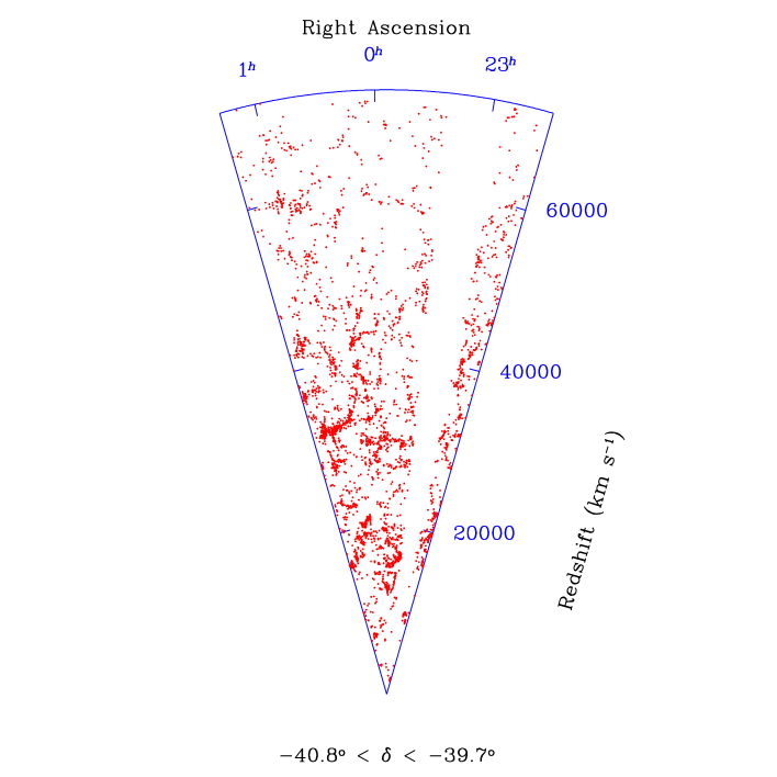
Figure 2: The distribution of galaxies within the 1-degree slice of the ESP survey (the gap around $23^{h}$ corresponds to a region that was not observed).

This reasoning was at the origin of the ESO Slice Project (ESP) redshift survey, which used the ESO Optopus fibre coupler to observe all objects in the EDSGC down to $b_{J}=19.4$ within a thin strip of $\sim 1^{\circ}\times 26^{\circ}$, constructing an 85% redshift–complete sample of 3348 galaxies. The step forward in depth was gigantic, with respect to the Zwicky–based surveys, nearly 4 magnitudes, which lead to an effective survey depth corresponding to a luminosity distance of $\sim 600{\rm\mskip 5.0mu plus 5.0muh^{-1}\,Mpc}$. A pictorial view of the large-scale distribution of galaxies in the ESP is shown in the cone diagram of Figure 2. The survey and the main results obtained from its analyses have been largely discussed in a series of papers [26, 27, 28, 29, 30, 31, 32]. I shall summarise the main results obtained on galaxy clustering in the ESP survey in §5.

Also based on intensive use of a multi–object fibre spectrograph, is the largest redshift survey completed to date, i.e. the Las Campanas Redshift Survey (LCRS [33]), which represents the best existing compromise between depth and angular aperture. This redshift catalogue is slightly less deep than the ESP ($r<17.7$, roughly corresponding to $b_{J}\sim 18.8$ for a typical mean galaxy colour), but covers six slices of $\sim 80^{\circ}\times 1.5^{\circ}$, for a total of $\sim 26,000$ redshifts. Unlike most of the aforementioned surveys, the photometric parent sample for the LCRS was constructed anew from a specifically performed CCD drift–scan survey in the $r$ band.

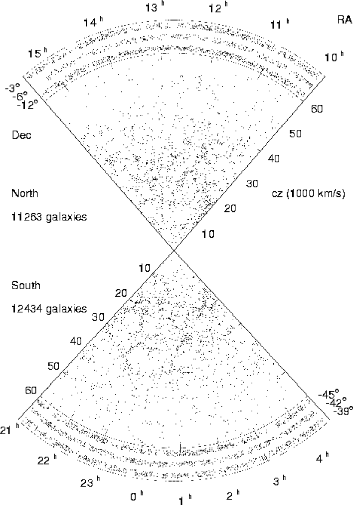
Figure 3: The famous double–cone diagram from the Las Campanas Redshift Survey. Both cones show galaxies projected from three adjacent RA slices of $1.5^{\circ}$ each [33].

One peculiarity of the LCRS is that the selection of the target galaxies was subject not only to a cut in apparent magnitude, but also to a selection in surface brightness within the aperture of the used fibres. It is now clear (Dalcanton, private comm.), that this selection favours bulge–dominated galaxies, preferentially excluding the irregular galaxies that represent the main population at faint luminosities. This has a clear effect on the galaxy luminosity function as measured from the LCRS, showing up in an abnormally flat faint end [34], (see [27] for comparison to other surveys). On the other hand, the global clustering properties do not seem to be significantly affected by this selection, as judged from the comparison of its two–point correlation function with those of the ESP and Stromlo–APM surveys ([32], see also Figure 9 hereafter). The double cone diagram showing the large–scale distribution of galaxies in the six LCRS slices is reproduced in Figure 3.

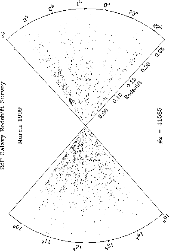
Figure 4: The distribution of the 41585 galaxies observed so far (March 1999)in the 2dF survey: like light beams through a smoky room, the 2dF observations are steadily unveiling the details of large–scale structure, at a typical rate of $\sim 2000$ redshifts per observing night. (Courtesy of the 2dF team).

The advantages of multi–object fibre spectroscopy have been pushed to the extreme with the construction of the 2–degree–Field (2dF) spectrograph for the prime focus of the Anglo–Australian Telescope [35]. This instrument is able to accommodate 400 automatically positioned fibres over a 2–degree–diameter field. This implies a density of fibres on the sky of $\sim 130$ deg^-2, and an optimal match to the galaxy counts for a magnitude similar to that of the ESP survey, $b_{J}\simeq 19.5$. The striking difference is that with such an area yield, a number of redshifts as in the ESP survey (although not distributed over a strip) can be collected in $\sim 10$ exposures, i.e. slightly more than one night of telescope time with typical 1 hour exposures! It was rather natural, therefore, that a large redshift survey based on the 2dF spectrograph were proposed by a UK-Australian team. This survey is now known as the 2dF galaxy redshift survey, and is based on the APM catalogue, giving us one further example of how importance of such large photometric catalogues. Its goal is to measure redshifts for more than 250,000 galaxies with $b_{J}\leq 19.5$. About 4/5 of these lay within two large areas, $75^{\circ}\times 12.5^{\circ}$ and $65^{\circ}\times 7.5^{\circ}$ within the South and North Galactic Caps respectively, which are being fully covered with a honeycomb of 2dF fields. Another 40000 redshifts will be measured within 100 fields randomly distributed over the APM area, with the goal of maximising the signal in the power spectrum estimate on very large scales [36]. In addition, a faint redshift survey of 10,000 galaxies brighter than $R=21$ will be performed over selected fields within the two main strips. The survey is steadily collecting redshifts, and first results on the luminosity function for different morphological types (defined through their spectral properties), have been recently presented [37]. From the cone diagram of Figure 4, we can have a visual impression of the status of the survey as of March 1999, with a total of 41585 redshifts measured, (note that the thickness of the slice is not uniform over the RA range). With the eye trained by the ESP and LCRS diagrams, one can easily see the structures taking shape across the survey beams. More details can be found in [38], and [39]. See also the 2dF web page at http://msowww.anu.edu.au/$\sim$colless/2dF/, where the diagram of Figure 4 is continuously updated.

The most ambitious and comprehensive galaxy survey project currently in progress is without any doubt the Sloan Digital Sky Survey (SDSS). This massive effort is carried on by an American consortium with the participation of Japan. Aim of the project is first of all to observe photometrically the whole northern galactic cap, $30^{\circ}$ away from the galactic plane ($\sim 10^{4}$ deg²) in five bands, at limiting magnitudes, respectively of $u^{\prime}=22.3$, $g^{\prime}=23.3$, $r^{\prime}=23.1$, $i^{\prime}=22.3$ and $z^{\prime}=20.8$. The expectations are to detect $\sim 5\times 10^{7}$ galaxies and $\sim 10^{8}$ star–like sources among which a subset of $10^{6}$ AGN candidates can be selected by colour techniques. This has already led, based on the first few hundred deg² covered since first light (May 1998), to the discovery of several high–redshift ($z>4$) quasars, including the highest–redshift quasar known, at $z=5.0$ [40]. Using two fibre spectrographs carrying 320 fibres each, the spectroscopic part of the survey will then collect spectra for about $10^{6}$ galaxies with $r^{\prime}<18$ and $10^{5}$ AGN’s with $r^{\prime}<19$. The spectrographs are still being commissioned at the telescope at the time of writing this paper (Spring 1999).

The capability to isolate photometrically sub–classes of objects through their colours will be exploited also by selecting a sample of about $10^{5}$ “red” luminous galaxies with $r^{\prime}<19.5$. These will be observed spectroscopically providing a nearly volume-limited sample of early–type galaxies with a median redshift $z\simeq 0.5$, that will be extremely valuable to study the evolution of clustering. In Figure 5, using a numerical simulation, the expected power spectrum of the whole SDSS spectroscopic galaxy survey (bottom line) is compared to that corresponding to the subsample of red luminous galaxies [41]. Note the gain in the clustering signal around the turnover in the power spectrum.

It is clear from this short description how the goals of the SDSS are well beyond the pure realisation of a redshift survey for just studying large–scale structure. Indeed, in addition to the immediate scientific results that will be produced by the survey team, it will build an unparalleled photometric and spectroscopic data base whose impact on the scientific community will last for several years. Further details can be found in [42], with a more recent update as of fall 1998, in [41]. See also the SDSS web site at http://www.sdss.org/, where the latest news on the ongoing survey can be found.

Figure 5: Expected $1\sigma$ accuracy in the galaxy power spectrum measured from the SDSS data. The solid lines give the (input) power spectrum. The bottom curve is for the 900,000 galaxies expected in the main survey volume to $r^{\prime}<18$, while the top curve is for the deeper subset of 100,000 red luminous galaxies with $r^{\prime}<19.5$ (Loveday 1998).

3 A Fair Sample of the Universe?

A general impression one could draw from the cone diagrams of the ESP and LCRS surveys, and which is also taking shape within the 2dF preliminary plot, is that inhomogeneities in the distribution of galaxies are limited to scales of $100-200{\rm\mskip 5.0mu plus 5.0muh^{-1}\,Mpc}$, which are fairly well covered by these modern surveys. Using Bob Kirshner words, we seem to be finally seeing “the end of greatness”, that is, we are finally sampling (at least in two dimensions) sizes which contain the relevant clustering scales of our Universe. This was not the case until a few years ago, when any new survey used to discover larger and larger structures. A clear example of this situation is provided by the combined CfA2–SSRS2 sample that we have shown in Figure 1. Here the largest superclusters have sizes $\sim 150{\rm\mskip 5.0mu plus 5.0muh^{-1}\,Mpc}$, comparable to the survey depth, and spanning its volume from one side to the other.

It was because of evidences like these, together with the power–law behaviour shown by galaxy clustering (see §5.1), that some researchers suggested that the large–scale galaxy distribution of galaxies could be described as a “fractal dust” (e.g. [43]). This fractal behaviour, if extrapolated to indefinite scales, i.e. if not up–bounded by a transition to a homogeneous distribution, has some rather dramatic consequences on our statistical description of large–scale structure [44]. No mean density can be defined, and as a consequence the whole concept of density fluctuations (with respect to a mean density) becomes nonsensical.

A quite intense debate has developed in the last few years about whether the available surveys really provide evidence for homogeneity on the largest scales explored, with – as it often happens – a tendency of the opposing views to crystallize on polarized positions. As an attempt to clarify a bit the situation by addressing this very basic question in a possibly objective way, in [45] I reviewed some of the best available redshift survey data from this point of view. The application of some simple counting statistics, corroborated also by other more detailed analyses [46, 30], seemed to show a general convergence to a homogeneous distribution, rather than supporting a fractal behaviour to the largest explorable scales. At the same time, however, it was clear (as previously remarked [47]), that the clustering of galaxies on small and intermediate scales could be described by power–law ranges consistent with a fractal, scale–free distribution. Similar conclusions have been reached more recently by Martinez [48].

3.1 Density Fluctuations and Variances

Once we are convinced that indeed a transition to homogeneity does exist on some large scale around $\sim 100-200{\rm\mskip 5.0mu plus 5.0muh^{-1}\,Mpc}$ so that we can define a mean density of the Universe in a sensible way, we can quantify the distribution of objects and matter in terms of density fluctuations. Given a mean density $n$, and a spherical volume of radius $R$, we can measure the fluctuation $\delta N/N$ in the number of objects within such spheres, and compute the variance $\sigma^{2}_{gal}(R)$ of this quantity. We shall then find that for typical optically–selected samples this is a decreasing function of $R$ (galaxies are indeed clustered!), with $\sigma^{2}_{gal}\simeq 1$ for $R=8-10{\rm\mskip 5.0mu plus 5.0muh^{-1}\,Mpc}$, depending slightly on the mean luminosity of the objects considered. In particular, modern redshift surveys, with typical sizes exceeding a few $100{\rm\mskip 5.0mu plus 5.0muh^{-1}\,Mpc}$, are probing volumes of the Universe over which $\sigma^{2}_{gal}$ is significantly smaller than unity.

Unless mass is more clustered than light, this should be reflected by a similar or even smaller variance $\sigma^{2}_{\rho}$ in the mass density fluctuation field $\delta\rho/\rho$. When $\sigma_{\rho}<1$, linear perturbation theory can be applied and comparison of models to observations becomes easier. In fact, if clustering is driven by gravitational instability, the amplitude of perturbations in the linear regime grows with time in a way which is independent of the spatial wavelength of the perturbation itself (see e.g. [49], [50], [51]). For this reason, the evolution of any statistics describing the distribution of amplitudes at different wavelengths, as is the case for the power spectrum $P(k)$, and to some extent also of its Fourier transform the two–point correlation function $\xi(r)$ , will be described by a simple growth in amplitude, without any change in the shape.

This means in practice that if we are able to measure accurately the present shape of $P(k)$ or $\xi(r)$ on scales where this behaviour still holds, we have a direct probe of the initial distribution of fluctuations, which can be directly compared to the linear power spectra predicted by the different models. This is one of the main motivations for extending redshift surveys to larger and larger volumes of the Universe.

3.2 Mapping Light, Mapping Mass

In the previous paragraph, we have quickly touched on the possibility that the variances we observe in the distribution of light and mass are not strictly the same. In fact, as we discussed, whatever redshift survey we are performing, we are not mapping the distribution of mass in the Universe, but rather the distribution of objects that can be “seen” in some band of the electromagnetic spectrum and that serve as possible tracers of matter distribution. We have seen, for example, that the LCRS and ESP are selected in different photometric bands, red and blue respectively, with a further important cut in surface brightness for the LCRS, and how these differences affect measured properties as the luminosity function [27].

While the LCRS and ESP galaxies do not show significant variations in the global clustering properties (i.e., they apparently trace the density field in similar ways), more serious differences are found for example between optically–selected and infrared–selected samples, as notably shown by the large surveys based on the IRAS satellite infrared survey. A selection based on the IRAS infrared flux favours star-forming galaxies and avoids rich clusters. Consequently, the IRAS density field is smoother than that generally seen by optically–selected galaxies, with a smaller correlation length ($\sim 3{\rm\mskip 5.0mu plus 5.0muh^{-1}\,Mpc}$ vs. $5{\rm\mskip 5.0mu plus 5.0muh^{-1}\,Mpc}$). Does this mean that IRAS galaxies trace the mass density field, i.e., that they are unbiased objects? The only way to answer this question is to compare the galaxy distribution to the mass distribution derived independently from dynamical observations of the peculiar velocity field (see e.g. [54]) and for the case of IRAS galaxies, the answer is probably yes.

To further clarify what we mean by biased tracers, let us have a look at the distribution of different morphological types. It is well known that different galaxy types find themselves preferentially within different density regimes: elliptical and S0’s favour high–density regions, while spirals are much more common in low–density environments. This is the so–called morphology–density relation (e.g. [55]), and it inevitably affects the way in which different types trace the underlying mass density field. In Figure 6 I have included an estimate of the real–space two–point correlation function $\xi(r)$ for early– and late–type galaxies, obtained from the projected function $w_{p}(r_{p})$ [56]. The plot shows how the morphology–density relation translates into a stronger clustering for elliptical galaxies. So, if we were for some reason able to detect only elliptical galaxies and assumed that they trace the mass, we would at first glance conclude that matter in the Universe is on the average more clustered than it really is.

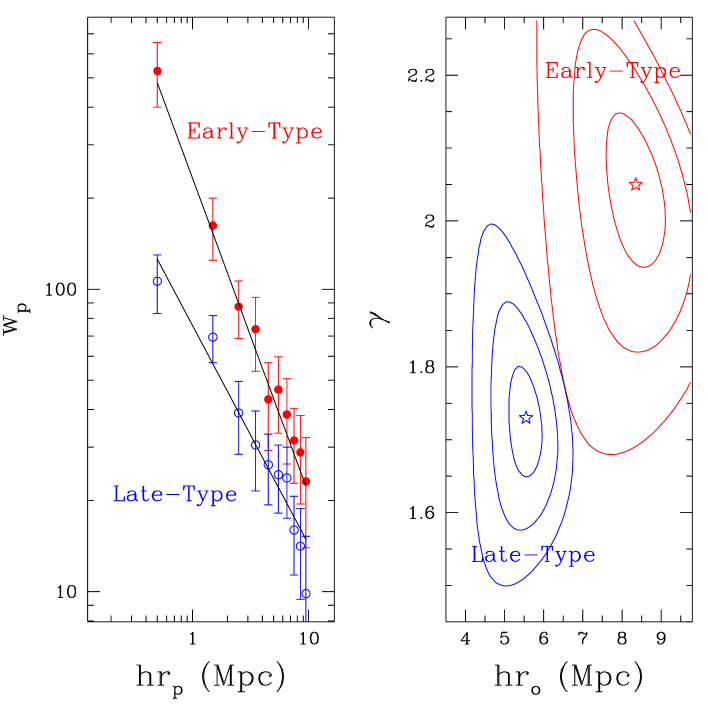
Figure 6: Comparison of the spatial correlation functions of early– and late–type galaxies. The left panel shows the so–called projected correlation function $w_{p}(r_{p})$, i.e. a projection of galaxy correlations perpendicular to the line of sight which has the advantage of being free from the distortions induced by peculiar velocities (see e.g. [56] for details). The right panel gives the confidence ellipses for the values of the correlation length $r_{o}$ and slope $\gamma$, when a power-law spatial correlation function $\xi(r)=(r_{o}/r)^{\gamma}$ is fitted to the data. Clearly, early–type galaxies (ellipticals and S0’s) are significantly more clustered than late–types (spirals and irregulars). So, which sort of galaxies (if any) are really tracing the large–scale mass density field?

All these examples pertain to the grand challenge of understanding how radiation emitted by cosmic objects (at any wavelength) is related to mass, i.e. the so–called bias, and even more importantly how this relation evolves with cosmic time. One way to define this is to write that

$$\sigma_{gal}(R)=b\,\sigma_{\rho}(R)\,\,\,\,\,,$$ (1)

where the linear bias $b$ is in general a function of scale $R$ and time $t$. A proper comprehension of the behaviour of $b(r,t)$ is becoming crucial now that observational data on clustering at very different cosmic epochs are being accumulated (e.g. [57]). For this reason, considerable energy has been spent in the last couple of years in developing physically motivated bias models (e.g. [58, 54, 59]).

4 Clusters of Galaxies as Tracers of Large–Scale Structure

With mean separations $>10{\rm\mskip 5.0mu plus 5.0muh^{-1}\,Mpc}$, clusters of galaxies are ideal objects for sampling efficiently long–wavelength fluctuations over large volumes of the Universe. Furthermore, fluctuations in the cluster distribution are amplified with respect to those in galaxies, i.e. they are biased in much the same way as we were discussing previously some classes of galaxies are: rich clusters form at the peaks of the large–scale density field, and their variance is amplified by a factor that depends on their mass, as it was first shown by Kaiser [60]. In the next section we shall see explicitly this effect at work in recent analyses of the clustering of clusters.

A thorough review of the use of clusters as tracers of large–scale structure has been given recently by Postman [61], with particular attention paid to optically–selected clusters. For this reason, I will not discuss here the important issue of selecting clusters of galaxies in the optical band, i.e. from the 2D distribution of galaxies on the sky, but I will concentrate on results from X-ray selected cluster samples. Reference to optically–selected samples will be limited to a discussion of the clustering results obtained from them.

Studies of X-ray selected clusters date back to the beginning of X-ray astronomy [62]. However, only in recent years statistical studies became feasible, although still limited to the study of the temperature and luminosity functions, in particular through the data from the Einstein Medium Sensitivity Survey [63, 64]). The ROSAT satellite, launched in 1990, not only produced serendipitous samples of distant clusters to update these studies (see [65] for a review), but carried out the first all–sky survey ever with an X-ray imaging telescope. This has represented a tremendous input for studies of large–scale structure using clusters of galaxies, as I shall describe in this section.

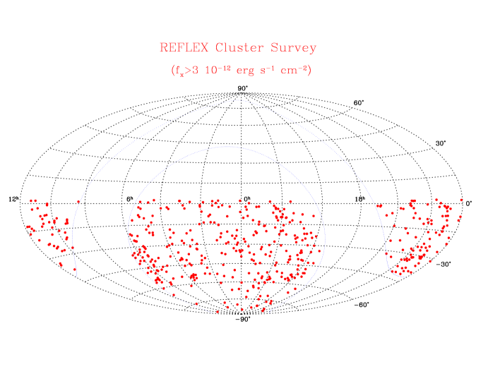
Figure 7: The distribution on the sky of the 460 X-ray clusters in the REFLEX survey, to $f_{x}>3\times 10^{-12}$ erg s^-1 cm^-2.

The ROSAT All-Sky Survey (RASS) was performed in the energy band between 0.1 and 2.4 keV with the PSPC, a photon counter with a $\sim 20$ arcsec resolution on axis, degrading to nearly 2 arcmin at the edges of the 2–degree field of view [66]. The median exposure time in the RASS was of $\sim 300$ s, which translates in an effective detection limit for clusters of $\sim 10^{-12}$ erg s^-1 cm^-2. Considering that in the ROSAT hard band (0.5–2.0 keV), $L^{*}\simeq 1\cdot 10^{44}$ h^-2 erg s^-1 [67], this detection limit translates into a typical depth of $d_{L}\simeq 900{\rm\mskip 5.0mu plus 5.0muh^{-1}\,Mpc}$, i.e. $z\simeq 0.3$. The RASS, therefore, provides a unique opportunity to detect clusters of galaxies within a huge volume of the “local” Universe.

In fact, follow–up work to construct X-ray cluster samples from the RASS and measure their redshifts started early after completion of the survey (see [68] for a review). A first example was a survey in the SGP area, that constructed a sample of about 200 clusters with the main aim of measuring the cluster–cluster correlation function [69]. Only recently, however, the all–sky coverage of the RASS was properly exploited. This has been the aim of the ROSAT-ESO Flux Limited X-ray (REFLEX) cluster survey, that uses clusters of galaxies to explore, in the Southern hemisphere, a volume of the Universe comparable to that of the SDSS.

4.1 The REFLEX Survey

The REFLEX cluster survey combines the X-ray data from the RASS and optical follow–up observations using the ESO telescopes, to construct a complete sample of about 700 clusters with measured redshift, to a flux limit $f_{x}\simeq 1.5\times 10^{-12}$ erg s^-1 cm^-2 in the ROSAT band (0.1–2.4 keV). The survey covers essentially the southern celestial hemisphere ($\delta<2.5^{\circ}$), at galactic latitudes $|b_{II}|>20^{\circ}$, to avoid regions of high absorption and crowding by stars.

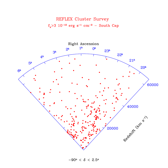
Figure 8: The large–scale distribution of X–ray selected clusters in the REFLEX survey. Only the South Galactic Cap part of the survey is shown here.

During the development of the survey, this project already produced a first bright sample of 135 clusters (the RASS1 bright sample [70]), limited to the SGP area, that served as a pilot work to fine–tune the strategy. At the time of writing (Spring 1999), the first REFLEX sample of nearly 460 objects with $f_{x}>3\times 10^{-12}$ erg s^-1 cm^-2 is on the verge of completion. This first sample, upon which the results on clustering and large-scale structure presented in the next sections are based, has been constructed to be at least 90% complete [71]. Several external checks, as comparisons with independently extracted sets of clusters, support this figure. 95% of the candidates in this sample are confirmed and observed spectroscopically, while all redshifts should be measured by the summer of this year. The distribution on the sky of the REFLEX clusters in this complete sample is shown in Figure 7, while their 3D distribution can be appreciated from the cone diagram of Figure 8. From this latter figure we can see how at this flux limit, the depth of the REFLEX survey is similar to that of the most recent galaxy surveys, as 2dF the and SDSS. At the same time, given the large solid angle of REFLEX, only the SDSS will be able to explore a comparable volume. Of course, clusters provide a coarse–resolution mapping of structures with respect to galaxies, but it is a price one is happy to pay, as in parallel extremely large scales can be explored with a reasonable investment of telescope time.

5 Statistics of Large-Scale Structure

In the previous sections we have mostly limited our discussion to the observed general characters of the large–scale structure of the Universe within $z<0.2$, as described by the distribution of luminous objects. The visual appearance of large–scale structures – while very interesting per se – needs to be translated into a quantitative description through the application of statistical estimators of clustering if one wants to compare the data to model predictions.

The increased size of galaxy and cluster redshift samples that we have discussed in the previous sections, has in parallel given the possibility to produce more and more accurate estimates of the two–point correlation function and the power spectrum of the distribution of these objects. This has allowed us to start looking at the details of the shape of these functions, in particular on large scales, where we have seen they are more interesting for the theory. Such details, if confirmed, can have profound consequences for our understanding of the origin of large–scale structure, as I shall try to summarize and discuss in this section.

5.1 The Galaxy Two–Point Correlation Function

The simplest approach to clustering is to ask how much does it differ from a uniform distribution at the two–point level, or in other words, which is the excess probability over random to find a galaxy at a separation $r$ from another galaxy. This is one way in which the two–point correlation function $\xi(r)$ can be defined (see [72] for a more detailed introduction). The first estimates of the two–point correlation function go back to the seventies [73], but the lack of large redshift samples limited these early analyses to the angular correlation function $w(\theta)$. This is related to $\xi(r)$ through the Limber equation [72]

$$w(\theta)=\int_{0}^{\infty}dy\,y^{4}\,\phi^{2}\int_{-\infty}^{\infty}dx\,\xi\left(\sqrt{x^{2}+y^{2}\theta^{2}}\right)\,\,\,\,\,,$$ (2)

where $\phi$ is the radial selection function expected for the 2D survey being analysed.

The basic description of galaxy clustering that emerged from these works is still valid today on small and intermediate scales: $w(\theta)$ is well described by a power law $\propto\theta^{-0.8}$, corresponding to a spatial correlation function $(r/r_{o})^{-\gamma}$, with $r\simeq 5{\rm\mskip 5.0mu plus 5.0muh^{-1}\,Mpc}$ and $\gamma\simeq-1.8$, and a break with a rapid decline to zero around $r\sim 10-20{\rm\mskip 5.0mu plus 5.0muh^{-1}\,Mpc}$. As we shall discuss in the following, modern surveys have significantly improved our knowledge of the two–point correlation functions especially on scales $>10{\rm\mskip 5.0mu plus 5.0muh^{-1}\,Mpc}$. However, before discussing these most recent results, it is important to briefly describe how galaxy peculiar velocities affect the observed shape of $\xi(r)$ .

5.1.1 REDSHIFT SPACE DISTORTIONS

The actual detection of true intrinsic deviations of $\xi(s)$ from a power law is complicated in the analysis of redshift surveys by the effects induced by galaxy peculiar velocities. Here $s$ is now used to make it explicit that separations are in reality not measured in true 3D space, but in redshift space: what we actually measure when we take the redshift of a galaxy is the quantity $cz=cz_{\rm true}+v_{\rm pec//}$, where $v_{\rm pec//}$ is the component of the galaxy peculiar velocity along the line of sight. This component, while typically $\sim 100\,{\rm km\,s^{-1}}$ for “field” galaxies, can rise above $1000\,{\rm km\,s^{-1}}$ in rich clusters of galaxies. This distorts the real–space correlation function in different ways, depending on the scale. The resulting $\xi(s)$ , is in general flatter than the real–space $\xi(r)$ . This is the result of two competing effects: the small–scale pairwise velocity dispersion, mostly dominated by high–velocity pairs in clusters of galaxies (i.e. those within the so–called “Fingers of God”), damps the amplitude of $\xi(r)$ below $\sim 3{\rm\mskip 5.0mu plus 5.0muh^{-1}\,Mpc}$. On the other hand, coherent flows towards large–scale structures enhance the contrast of those structures lying perpendicularly to the line of sight, thus amplifying $\xi(s)$ in the linear regime (i.e. above $10-20{\rm\mskip 5.0mu plus 5.0muh^{-1}\,Mpc}$). I will not enter here into details on how the wealth of information on the dynamics of galaxies contained in these distortions can be extracted, but limit myself to a discussion on how to correct them to recover the true shape of $\xi(r)$ . A more complete discussion can be found, e.g., in [74] and [51].

Redshift space distortions can be corrected either at a rough level, through a simple statistical compression of the “Fingers of God” (e.g. [75]), or in a more appropriate way by computing the correlation function $\xi(r_{p},\pi)$ , where the separation vector s between two objects is split into two components $r_{p}$ and $\pi$ related as $s^{2}=r_{p}^{2}+\pi^{2}$. This two–dimensional correlation function can then be projected along the line–of–sight direction, to obtain the function

$$w_{p}(r_{p})=\int_{0}^{\infty}\xi(r_{p},\pi)\,d\pi\,\,\,\,\,,$$ (3)

which is independent of redshift–space distortions. We have already encountered this function in Figure 6 when comparing the clustering strength of early– and late–type galaxies in real space (and thus free of their rather different peculiar velocity fields). $w_{p}(r_{p})$ can either be used to constrain the parameters of a chosen model for $\xi(r)$ , as e.g. the classical $\xi(r)=(r/r_{o})^{-\gamma}$ [56], or inverted through the Abel integral relations to recover the whole $\xi(r)$ .

All these problems are obviously absent when one analyses $w(\theta)$, where on the other hand the strongest uncertainty in the de–projection lies in the knowledge of the radial selection function.

5.1.2 THE LARGE–SCALE SHAPE OF $\xi(r)$ 

The simple form observed from the first estimates of $w(\theta)$ and $\xi(r)$ at small separations was consistent with the expectations of gravitational growth from some initial spectrum of fluctuations (at the time thought to possibly be a simple white–noise i.e. $\propto k^{0}$, see next section): as gravity has no built–in preferential scale, a power law seemed to be a natural consequence of gravitational clustering (see e.g. [72]). However, since then we have understood that plausible initial conditions are all but a white–noise (see e.g. the first computation of the linear power spectrum in a Universe dominated by Cold Dark Matter, [76]), so that the clustering we measure today with $\xi(r)$ is not just the product of the nonlinear action of gravity.

In Figure 9, I have plotted the estimates of $\xi(s)$ for the ESP [77, 32], the LCRS [78], the Stromlo–APM (Loveday et al. 1992b), and the Durham–UKST [80] surveys. These samples represent a selection of data that should offer the best compromise between depth and angular aperture, thus maximising the ability to sample large scales. In addition, the dotted lines show a plot of $\xi(r)$ obtained through de–projection of the angular $w(\theta)$ from the APM galaxy catalogue [81] under two different assumptions about galaxy clustering evolution and thus selection function.

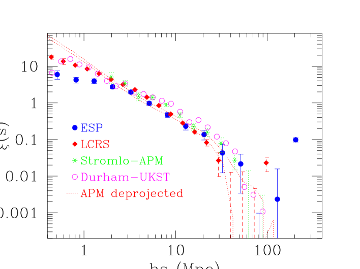
Figure 9: Recent estimates of the two–point correlation function of optically–selected galaxies. The plot shows results from the ESP (Guzzo et al. 1998, 1999), the LCRS (Tucker et al. 1997), the APM-Stromlo [79] and the Durham-UKST [80] surveys.

We clearly see how, within some scatter among different surveys, $\xi(s)$ remains positive to separations of $50{\rm\mskip 5.0mu plus 5.0muh^{-1}\,Mpc}$ or larger. Keeping in mind how the variance in galaxy counts is $\sim 1$ around $8{\rm\mskip 5.0mu plus 5.0muh^{-1}\,Mpc}$, we can conclude that a significant range of scales over which we measure positive clustering is still in the linear or quasi-linear regime.

The global form below $5-10{\rm\mskip 5.0mu plus 5.0muh^{-1}\,Mpc}$ is still well described by a power law: the slope is very close to the classical $-1.8$ for the APM $\xi(r)$ , which is in real space, while it is flatter for all the redshift–space measures due to the suppression by peculiar velocities discussed above. Above $\sim 5{\rm\mskip 5.0mu plus 5.0muh^{-1}\,Mpc}$ there is unanimous evidence for more power than expected by a simple extrapolation of the small–scale slope. This “bump” or “shoulder” is evident both in the APM $\xi(r)$ and in the redshift–space measures, implying that it is not an effect of the expected redshift–space amplification by coherent flows [82]. We found clear early evidence for this excess when studying clustering in the Perseus–Pisces survey [47], and realised that it was present already in the published CfA1 data (as also noticed in [83]). At the time we suggested that it was and indication for a steep power spectrum $P(k)\propto k^{-2.2}$ on large scales. Further theoretical modeling [84] and the new direct measures of $P(k)$ in real space from the APM survey [85], confirmed that indeed there is a significant change in $\xi(r)$ around $r\simeq 3-5{\rm\mskip 5.0mu plus 5.0muh^{-1}\,Mpc}$. It was natural to interpret this as a consequence of the transition between the strongly nonlinear clustering regime at small separations, to a quasi–linear regime on larger scales. In §5.3 we shall come back to this point while discussing directly the observed shape of $P(k)$.

5.2 The Clustering of Clusters

We have seen that clusters of galaxies represent a powerful tracer of structure on the largest possible scales. Their clustering can be also quantified at the simplest level through the two–point correlation function. The classic estimate of $\xi(s)$ for Abell clusters [86] showed that the cluster–cluster correlation function is also well described by a power law, with a slope apparently similar to that of galaxies, but a correlation length about 4 times larger. In reality, due to the limited size of the sample, the original fit was performed imposing a slope $\gamma=1.8$, and therefore it was not really a measure of the functional shape of cluster–cluster correlations. Nevertheless, the fit was good enough, and it became generally accepted that the cluster-cluster correlation function has a the same slope as galaxies, $\gamma=1.8$, but larger amplitude (see e.g. [60]), that is $\xi_{cc}(r)\simeq A\cdot\xi_{gg}(r)$. In fact, this statement could not rigorously be true if a simple statistical amplification mechanism, as then suggested by Kaiser [60], were the origin of the different amplitude: clusters trace scales $>10{\rm\mskip 5.0mu plus 5.0muh^{-1}\,Mpc}$, i.e. cover mostly fluctuations that are in the quasi–linear or linear regime, and it would have been a rather strange conspiracy, that their slope were the same that galaxies display on scales between 0.1 and $5{\rm\mskip 5.0mu plus 5.0muh^{-1}\,Mpc}$, where clustering is highly nonlinear.

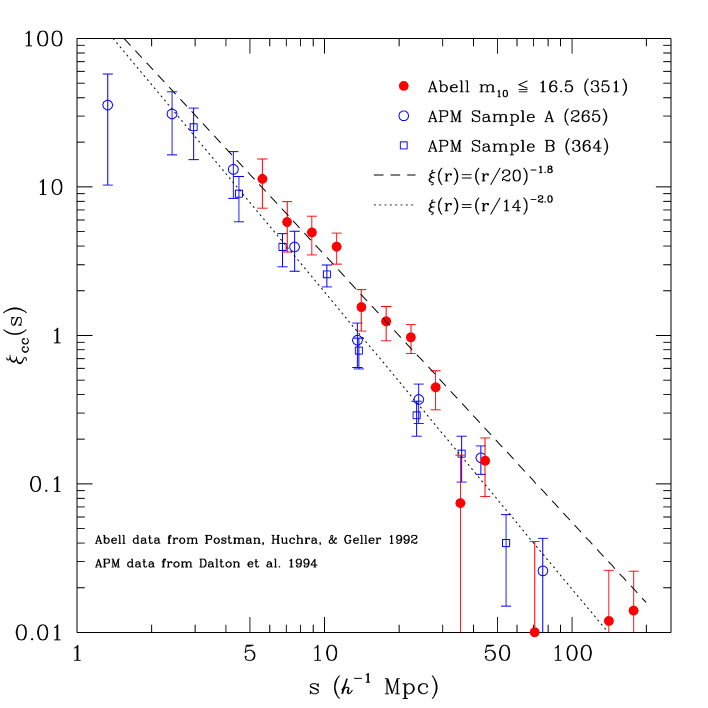
Figure 10: The cluster–cluster correlation function optically–selected clusters from the Abell and APM catalogues, reproduced from the review by Postman [61].

The basic problem was that the galaxy correlation function was not known accurately enough on large scales, as to provide a meaningful comparison. The situation has fortunately improved significantly since then. We have just reviewed the significant progress made in our knowledge of the galaxy correlation function. In parallel, new cluster samples have been constructed, such as the EDCC [87] and APM [89] automatically selected cluster catalogues, and the quality and number of redshifts available for Abell clusters have substantially increased.

Although I will not enter into details concerning optically–selected clusters, in Figure 10 I have reproduced a plot from [61], showing an up–to–date comparison of the cluster–cluster correlation functions of both an Abell sample [88], and a sample of APM clusters [89]. While comparison is presented with two possible power laws, the data clearly show a break from these simple models around $50{\rm\mskip 5.0mu plus 5.0muh^{-1}\,Mpc}$, much in the same way as galaxies do on a similar scale. See [61] for more details.

In section §4.1 I argued that X-ray selection is the best way to select homogeneous samples of clusters with well–defined physical criteria out to large redshifts. In particular, X-ray luminosity is a parameter that is much more closely related to mass than the somewhat loosely defined richness, used to characterise optically–selected clusters. For this reason, model predictions for the clustering of massive objects, can be more easily and safely translated in terms of observable quantities as luminosities and fluxes, than in the case of galaxies [90]. At a simpler observational level, it is particularly interesting to compare $\xi_{cc}$ for X-ray selected clusters to that of galaxies, as we do in Figure 11 [91]. This figure shows a preliminary estimate of $\xi_{cc}$ from the flux–limited REFLEX survey [92], compared to the galaxy–galaxy correlation function from two volume–limited subsamples of the ESP survey [32] . The dashed line on top of the cluster points is the Fourier transform of the power spectrum of REFLEX clusters (computed independently, see next section) while the bottom line has been scaled down by an arbitrary factor $b_{cg}^{2}=(3.3)^{2}$, so as to overlap the galaxy points. The agreement between the shapes of the cluster and galaxy correlation functions is remarkable. Here we also see how a proper functional description of the shape is not just a simple power law. The one shown here is the Fourier transform of the simple phenomenological shape for $P(k)$suggested by Peacock [51].

The result shown in Figure 11 is a powerful confirmation of a simple linear bias model between galaxies and clusters of galaxies, analogous to eq. (1), as first suggested by Kaiser [60] (see also [93] for a more recent refinement). Indeed, considering the relationship between $\xi(r)$ and the variance within a top–hat sphere of radius $r$

$$\sigma^{2}(r)={1\over V_{r}}\int_{V_{r}}\xi(x)d^{3}x\,\,\,\,,$$ (4)

eq. (1) implies that the cluster and galaxy correlation functions obey to the relation

$$\xi_{cc}(r)=b_{cg}^{2}\xi_{gg}(r)\,\,\,\,,$$ (5)

where the relative bias factor $b_{cg}$ is related to the typical mass of the clusters considered [60]. This kind of investigation can be generalised to the study of the dependence of the correlation length on the sample limiting X–ray luminosity, for which also model predictions can be quite specific [93]. This will also be an important output of the REFLEX survey [92].

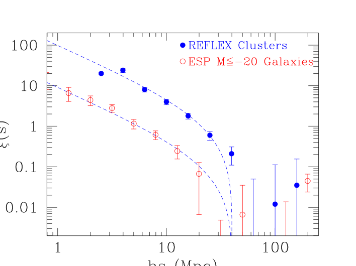
Figure 11: Comparison of the two–point correlation functions of REFLEX clusters [92] and ESP galaxies [32]. The top dashed line is the Fourier transform of a simple phenomenological fit of the REFLEX power spectrum with a double–power–law model. The bottom one is the same after scaling by an arbitrary bias factor of $b_{c}^{2}=(3.3)^{2}$. The agreement in shape between galaxies and clusters is remarkable. At the same time, both galaxies and clusters show an indication, after the breakdown around $r\simeq 50{\rm\mskip 5.0mu plus 5.0muh^{-1}\,Mpc}$, for more positive power on scales exceeding $100{\rm\mskip 5.0mu plus 5.0muh^{-1}\,Mpc}$.

5.3 The Power Spectrum

The Fourier transform of the correlation function is the power spectrum P(k)

$$P(k)=4\pi\int_{0}^{\infty}\xi(r){\sin(kr)\over kr}r^{2}dr\,\,\,\,\,,$$ (6)

which describes the distribution of power among different wavevectors or modes $k=2\pi/\lambda$ once we decompose the fluctuation field $\delta=\delta\rho/\rho$ over the Fourier basis [51].

The amount of information contained in $P(k)$ is thus formally the same yielded by the correlation function. The estimates of $P(k)$ or $\xi(r)$ from redshift surveys, however, are affected in different ways by uncertainties introduced, for example, by the poor knowledge of the mean density (in which case the power spectrum is to be preferred), or by the shape of the survey volume (whose effect is usually more easily treated when computing $\xi(r)$ rather than $P(k)$). Useful references for learning more about this topic are [94], [7] and [51], where further directions can be found to specific technical papers. One practical benefit of the description of clustering in Fourier space through $P(k)$ is that for fluctuations of very long spatial wavelength ($\lambda>100{\rm\mskip 5.0mu plus 5.0muh^{-1}\,Mpc}$), where $\xi(r)$ is dangerously close to zero and errors easily make the measured values fluctuate around it, $P(k)$ is on the contrary very large. Around these scales, most models predict the power spectrum to have a maximum, which reflects the size of the horizon at the epoch of matter–radiation equivalence.

Indeed, comparison of observations to the theory is in principle easier and more direct using $P(k)$. First, models are usually specified in terms of a linear $P(k)$, which is the result of the action of the specific transfer function of the model on a primordial spectrum, usually assumed to be of the so–called Harrison–Zel’dovic scale–invariant form $\propto k^{1}$, which is also the kind of spectrum most naturally produced in inflationary scenarios (see e.g. [50] for more details). In addition, k–modes in Fourier space are statistically independent (a part from the convolution effects due to the window function of the survey, see below), and direct $\chi^{2}$ comparisons to models is feasible, which is in principle not the case when the correlation function is analysed (see e.g. [95]).

However, not everything is better with power spectra. Redshift surveys are all but cubes (i.e. what would be optimal for a Fourier plane–wave decomposition), and their geometrical shape affects the measured power, so that what we really measure is the quantity

$$\tilde{P}({\bf k})=\int d{\bf k}^{\prime}\left|W({\bf k}-{\bf k}^{\prime})\right|^{2}\,P({\bf k}^{\prime})\,+\,SN\,\,\,\,\,\,.$$ (7)

The measured power spectrum is therefore a convolution of the true $P({\bf k})$ with the square modulus of the window function $\left|W({\bf k})\right|^{2}$, that is the Fourier transform of the survey volume, plus an additional shot–noise term. While the shot–noise contribution $SN$ is easily corrected for, the recovery of the true $P(k)$ necessarily involves a delicate de–convolution operation in $k$ space. While for nearly tridimensional surveys (as IRAS-based surveys [96, 97, 98], or the CfA2–SSRS2 [99], Stromlo–APM [100], Durham–UKST [101], and REFLEX surveys), the effect of the window function is mostly negligible, for nearly two–dimensional surveys as the LCRS or, even worse, the ESP, its effect is dramatic to very small wavelengths. The key point is that for slice surveys like ESP, the window function is very anisotropic, in particular it is extremely large along the direction perpendicular to the main plane of the survey. When the final estimate of $P(k)$ is computed by averaging over the whole $4\pi$ solid angle, this anisotropy brings contributions from different ${\bf k}$’s into the same averaged $k$ bin. It is important to keep these limitations in mind when one compares estimates of $P(k)$ from different surveys as we shall do here. A comprehensive discussion on different estimators for $P(k)$ and how to take these effects into account can be found in [102].

A different approach for dealing with surveys with peculiar shapes is otherwise that suggested by Vogeley & Szalay [103], using the so–called Karhunen–Loève transform. Rather than trying to correct the effect of the window function over the plane waves of the Fourier basis, the idea is to find a different set of orthonormal eigenvectors which are optimal given the survey geometry. The interesting quantities, as e.g. $P(k)$, are then projected on this basis, both for the data and for the models, and comparison is performed through a maximum likelihood analysis. Application of this method has been so far limited only to the 2D case [103]. A first application to the REFLEX data [105] is yielding promising results.

5.3.1 THE POWER SPECTRUM OF THE GALAXY DISTRIBUTION

In Figure 12, I have plotted the estimates of $P(k)$ for the same surveys as given in Figure 9. The four data sets allow me also to make a comparison of estimates from relatively tridimensional surveys (Stromlo–APM, Durham-UKST), to more bidimensional samples as the LCRS and ESP, the latter being in practice a single thin slice cut through the galaxy distribution. This means that the effect of the window function (and the need of a proper correction) on these data sets is very different. In addition, three of the four samples are selected in exactly the same photometric band, the blue–green $b_{J}$ (two, ESP and Durham–UKST are even constructed from the same catalogue, the EDSGC), the only exception being the $r$-band selected LCRS. This has the positive effect of reducing the relative biasing between the different samples, although some effect is possibly still present due to the different luminosity ranges covered.

In the same figure, I have also plotted (dashed line) $P(k)$ as reconstructed from the projected angular clustering of the APM galaxy catalogue [85]. This is clearly the only estimate which is free of redshift–space distortions. The effect of these is shown in particular by the slope above $\sim 0.3\rm\,h\,Mpc^{-1}$: an increased slope in real space (dashed line) corresponds to a stronger damping by peculiar velocities, diluting the apparent clustering observed in redshift space (all points).

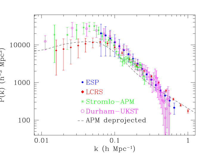
Figure 12: A non–exhaustive compilation of most recent estimates of the power spectrum of galaxy clustering, from four of the largest available redshift surveys of optically–selected galaxies (ESP [106]; LCRS [107]; Stromlo-APM [100]; Durham-UKST [101]), compared to that deprojected (and therefore in real space), from the 2D APM galaxy survey [85].

The first impression from this comparison is that to first order there is quite a good agreement across the different samples. The general trend is that of a well–defined power law range between $\sim 0.08$ and $\sim 0.3\rm\,h\,Mpc^{-1}$, with a slope around $k^{-2}$. Note that despite these samples are rather similar in terms of their galaxy properties, a minimal level of relative biasing might be present because of the relative weight of faint and bright objects. The only two samples that should in principle display the same amplitude are the ESP and the Durham–UKST surveys, which are both selected from the EDSGC catalogue. In fact, their $P(k)$ are practically identical over a good range of $k$’s. On one hand, the Durham–UKST $P(k)$ becomes rather noisy at small scales, due to the sparse sampling strategy of this survey (less sparse than the Stromlo–APM, though). On the other hand, the ESP $P(k)$ performs well on small scales, but on large scales it has to be limited to $k>0.06\rm\,h\,Mpc^{-1}$, below which the effect of its nasty window function cannot be deconvolved appropriately. In fact, the very good agreement with the Durham–UKST down to fairly small $k$’s is a very encouraging indication of the quality of the deconvolution procedure performed by the authors[106].

We also note how the LCRS power spectrum tends to be flatter and of lower amplitude around the tentative turnover displayed by the Durham–UKST and Stromlo–APM spectra. Also at large $k$’s, where ESP and Durham–UKST are significantly damped by small–scale pairwise velocities, the LCRS $P(k)$ seems to be less affected by this distortion. The same trend is also visible in the correlation function plot of Figure 9.

Recalling the discussion of § 5.1 on the shoulder observed in the two–point correlation function above $\sim 5{\rm\mskip 5.0mu plus 5.0muh^{-1}\,Mpc}$, here we can see clearly the same effect in $P(k)$ by looking at the real–space power spectrum from the APM catalogue. The slope of the APM $P(k)$ above $0.3\rm\,h\,Mpc^{-1}$ is $\sim k^{-1.2}$, corresponding to the small–scale clustering regime (in real space!) where $\gamma\simeq-1.8$. Below this scale, $P(k)$steepens to $\sim k^{-2}$, and this is what produces the excess power in $\xi(s)$ on large scales.

Peacock [108] applied the sophisticated linear reconstruction machinery by Hamilton and collaborators [109] to the whole $P(k)$ from the APM catalogue (and to another real–space estimate from the the IRAS-QDOT survey [110]) and concluded that the shape was indeed consistent with a linear power spectrum characterised by a steep slope ($\sim k^{-2.2}$). This is the same value of linear slope originally suggested in [47] to explain the observed large–scales shape of $\xi(s)$ in the CfA1 and Perseus–Pisces redshift surveys, and confirms the early speculation that the observed change in slope of $\xi(r)$ is a manifestation of the transition from the quasi–linear to the strongly nonlinear clustering regime.

5.3.2 THE POWER SPECTRUM FROM CLUSTERS

Also for measuring the power spectrum, clusters of galaxies offer the most efficient alternative to galaxies, given their ability to sample very large volumes. A first preliminary estimate of $P(k)$ from the REFLEX survey is shown in Figure 13 [105], compared to the power spectra of the largest redshift sample available for Abell clusters [111], and that of the APM automatic optically–selected clusters [112]. This is a conservative measure, based on only 188 of the nearly 460 clusters with redshifts that will form the final REFLEX sample, using a Fourier box of $400{\rm\mskip 5.0mu plus 5.0muh^{-1}\,Mpc}$ comoving side. This was done to avoid possible spurious fluctuations due to the incomplete sampling between the Northern and the Southern galactic sides of the survey. At the time of writing this review, virtually all clusters in the survey have been observed spectroscopically. A new measure of $P(k)$ in a box of $\sim 1000{\rm\mskip 5.0mu plus 5.0muh^{-1}\,Mpc}$ side (i.e. using all clusters within $z\sim 0.2$, where the survey is complete), should be produced by the end of 1999. Despite the point at smaller $k$’s is not significant, the turnover around $k\simeq 0.05\rm\,h\,Mpc^{-1}$ is shown to be significant at the $3\sigma$ level by a Karhunen-Loéve [103] Maximum Likelihood analysis. The analysis of the whole survey should also allow to put more serious constraints on the detailed shape of $P(k)$ around the turnover.

5.4 Features in the Power Spectrum

During the last few years, evidence has indeed been accumulating that the peak of the power spectrum could be rather sharp, perhaps characterised by an extra feature (with respect to smooth traditional models) around its maximum. Einasto and collaborators [114] analysed the distribution of Abell clusters, finding evidence for a sharp peak around $k\simeq 0.05\rm\,h\,Mpc^{-1}$. Although their result was questioned by other workers because of the possible incompleteness in the sample and the way $P(k)$ was estimated, the presence of such a feature was confirmed by a more conservative reanalysis of Abell data [111], where a slightly less pronounced but still significant peak is found, as we show in Figure 13. The peak is indeed evident in the Abell data, while the preliminary REFLEX sample is not yet able to put serious constraints on the shape around the turnover. Note also the very good agreement of the slopes of the three power spectra above $k\simeq 0.5\rm\,h\,Mpc^{-1}$, and at the same time the shift in amplitude of the three samples. The latter is a clear manifestation, again, of the different bias of the three samples. An X-ray selected sample as REFLEX allows for a more direct link to the typical mass of the objects we are looking at (see [115], for a more extended discussion of these points).

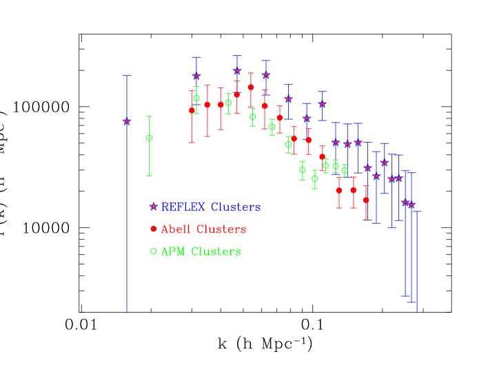
Figure 13: The power spectrum of the clustering of clusters, as measured from three different cluster surveys: a preliminary subsample of 188 clusters from the X-ray selected REFLEX survey [105], and redshift samples from the Abell [111], and APM [112] cluster catalogues. Note that a systematic difference in amplitude among these surveys is expected as they sample different mass thresholds, and are therefore characterised by different bias values.

If we also recall that evidence for excess power around $\sim 100{\rm\mskip 5.0mu plus 5.0muh^{-1}\,Mpc}$ was provided by a 2D power spectrum analysis of the LCRS slices [116], we cannot avoid being amused by the consistency in the peak scale to which these separate measures point, i.e., consistently between 100 and $150{\rm\mskip 5.0mu plus 5.0muh^{-1}\,Mpc}$. This is remarkably close to the “periodicity” scale revealed by Broadhurst and collaborators ([117], BEKS hereafter), in the analysis of their 1–dimensional pencil–beam surveys towards the galactic poles. This latter result has certainly been one of the most exciting findings of this decade in the study of large–scale structure. The authors merged together two deep redshift surveys of redshifts performed independently in the direction the two galactic poles over a small field of $\sim 0.7$ degrees, exploring a total 1–dimensional baseline of $\sim 2000{\rm\mskip 5.0mu plus 5.0muh^{-1}\,Mpc}$. The resulting galaxy distribution showed a surprising regularity of “spikes”. The visual impression was quantified and confirmed by a 1D correlation and power spectrum analysis, that clearly indicated a preferential “fluctuation” at $128{\rm\mskip 5.0mu plus 5.0muh^{-1}\,Mpc}$.

This result originated significant controversy. It was suggested that it could just be an aliasing of power due to the small size of the beam, that projected power from small to large scales [118]. On the other hand, the reality of the effect was supported by independent observations showing how the more nearby peaks detected in the pencil beam were coincident with known, real large–scale structures, as the Great Wall or the Sculptor supercluster (e.g. [119]). Further pencil beams in different directions (e.g. [120]), and a denser sampling around the original pointings [121] also show that, yes, this direction is somewhat special, but only in the sense that here the effect is maximised. This is what one would statistically expect if there is indeed a distribution of typical “cell” sizes around a characteristic dimension [122]. The peak observed in the 3D power spectrum of Abell clusters around the same scale is further suggesting that the origin of the BEKS periodicity lies indeed in a specific feature in the 3D power distribution around this wavelength.

Note also in Figures 9, 10 and 11 the behaviour of the two–point correlation functions on very large scales, for both galaxies and clusters. Although the binning of $\xi(s)$ is very coarse at these separations, there is a hint that $\xi(s)$ becomes positive again around $150-200{\rm\mskip 5.0mu plus 5.0muh^{-1}\,Mpc}$. This seems to be common to nearly all surveys, independently of their geometry (slice or 3D surveys), the kind of tracer (galaxy or clusters), and the estimator used. As can be readily seen by Fourier transforming a “standard” $P(k)$ (e.g., a CDM shape [123]), this damped oscillation of $\xi(s)$ cannot be reproduced if $P(k)$ has a smooth turnover around its maximum, and seems to be a further hint for a sharp peak. A similar oscillation in the correlation function was claimed for Abell clusters [124], and interpreted as evidence for a sharp feature in $P(k)$.

At the time of writing this review (Spring ’99), one very interesting piece of evidence has been provided along the same lines by Broadhurst and Jaffe [125], who analyse the redshift distribution of the high–redshift samples of Lyman–break selected galaxies by Steidel and collaborators [57]. As shown in Figure 14, they find again the same effect detected at smaller redshift, i.e. the emergence of a preferred clustering scale. One important consequence is that the co–moving scale of the peak in the power spectrum measured locally ($\sim 130{\rm\mskip 5.0mu plus 5.0muh^{-1}\,Mpc}$), can be used as a standard stick to provide a constrain on the combination of $\Omega_{M}$ and $\Omega_{\Lambda}$: $48\Omega_{M}-15\Omega_{\lambda}\simeq 10.5$, which for a flat Universe ($\Omega_{M}+\Omega_{\Lambda}=1$), gives $\Omega_{M}=0.4\pm 0.1$.

Figure 14: The one–dimensional clustering of Lyman–break galaxies, from [125]. Left: the co–added pair counts from 5 fields at $z\sim 3$ (top histogram), compared to the expectations from a randomly distributed sample with the same selection function (solid line). Right: the 1D correlation function along the line of sight, showing the clear pattern with $\sim 130{\rm\mskip 5.0mu plus 5.0muh^{-1}\,Mpc}$ periodicity (using $\Omega=0.2$). See [125] for details.

The convergence of so many independent observations seems to have left little doubt, in my opinion, that the observed characteristic scale is real, and is telling us something important about the properties of our Universe. Indeed, on the theory side there has been considerable interest in the recent literature about the possibile relation of this peak to baryonic acoustic features produced within the last scattering surface at $z\sim 1000$, when the Cosmic Microwave Background (CMB) radiation originated. Eisenstein and collaborators [126], show however how a large baryon fraction ($\Omega_{b}/\Omega_{o}\simeq 0.3$ or larger), and a rather ad hoc combination of parameters (as e.g. a “blue” tilt of the primordial spectrum) are required to match the observed Abell peak, while at the same time being consistent with the cluster abundance. More dramatically, it is worrying to see that no realistic CDM parameter combination is capable to account for the excess power (the “shoulder”) we were discussing in section 5.1, that is displayed by virtually all modern surveys [127].

Even without considering the existence of extreme features, therefore there seems to be a general difficulty for the “standard” theory to explain the detailed shape of $P(k)$, now that the data are becoming of higher and higher quality in the linear regime. Especially when one tries matching the power spectrum implied by the growing amount of CMB anisotropy experiments to that displayed by the clustering of luminous matter, problems seem to be unavoidable. According, for example, to Silk & Gawiser [128] “If the data are accepted as being mostly free of systematics and ad hoc additions to the primordial power spectrum are avoided, there is no acceptable model for large-scale structure.” Once again, a major uncertainty prevents any firm statement from being made: are we allowed to compare the power spectrum derived from the distribution of light to that derved from the mass (CMB), through a simple linear bias scaling? Clearly, a scale–dependent bias would add room for any detailed match between models and the data, but without a solid physical basis would also add an unpleasant ad hoc taste to the whole picture. In addition, the extremely linear relation between the correlation functions of galaxies and clusters that we have shown in Figure 11, seems to suggest that at least above $\sim 5{\rm\mskip 5.0mu plus 5.0muh^{-1}\,Mpc}$ the galaxy and mass distributions are linked by a simple linear bias.

6 Evolution of Large–Scale Structure

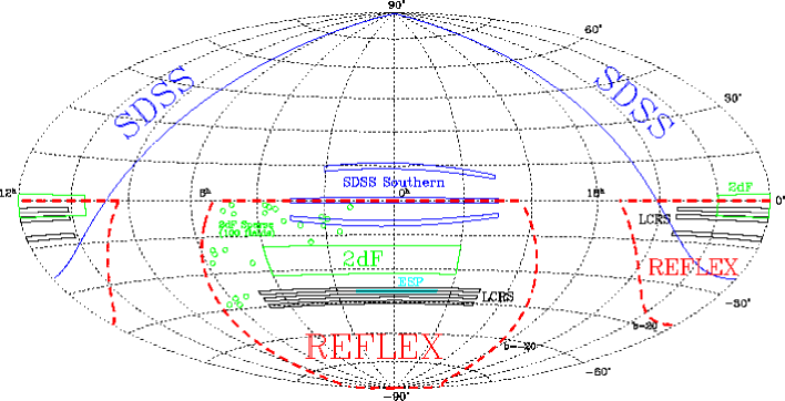
Figure 15: Pictorial view in Aitoff projection of the areas covered by the major galaxy and cluster redshift surveys discussed in the text.

Figure 15 gives a pictorial view of the sky coverage by wide–angle redshift surveys of galaxies and clusters that have mapped or are in the course of mapping the “local” Universe to $z\sim 0.2$. All these surveys have been discussed in some detail in the previous sections.

While considerable effort will still be necessary to complete the coverage both in photometry and redshift of this volume of the Universe, massive redshift surveys are already being planned to study large–scale structure at redshifts of the order of unity.

Deep redshift surveys, as demonstrated by the results from the clustering of Lyman–break galaxies discussed in the previous section, give in principle the possibility to trace the growth of structure, which represents a formidable test for theories: a successful model must be able not only to reproduce the final picture, but also all the snapshots of the “cosmic movie” at different epochs.

However, when we start exploring a baseline in time comparable to galaxy evolutionary times, we not only have the problem of understanding how our galaxy tracers map the underlying mass density field, but also to know the way they evolve, i.e. we need a full comprehension of the bias function $b(R,t)$. A successful theory must therefore provide two different ingredients: 1) a cosmological background, i.e. a linear power spectrum, depending on H_o, $\Omega$ and to the kind of dark–matter particles dominating the mass density, including a possible curvature contribution by a cosmological constant $\Lambda$ ; 2) a recipe to convert the mass and the growth history of “objects” (i.e. dark matter halos), forming during the gravitational evolution from the chosen initial conditions, into radiation with some spectral distribution, to be “observed” and compared to the real data. This is the arena of semi–analytical galaxy formation models (see the review by Kauffmann, these proceedings). Here halos obtained through analytical “merging trees” (e.g. [129, 130]), or from purely gravitational N–body simulations [131] are “lite–up” through as realistic as possible analytical recipes. This seems at present the best we can do to properly attach some “flesh” on the evolving “bones” of large–scale structure. It is self–evident that the inherent complication of realistically treating the dissipative part of this process (e.g. cooling, star formation, stellar evolution, supernova feedback – just to mention a few of the branches into which the problem of galaxy formation needs to be decomposed to become tractable), represents the weakest aspect of this machinery, and makes the use of galaxies as tracers of the evolution of large–scale structure a rather tricky game.

6.1 Non–Evolving Tracers?

Could we perhaps find a way to select some kind of tracer that does not evolve (or at least such that its evolution is weak and simple to understand), out to some cosmologically significant redshift? Clearly, if we push this redshift limit to some indefinitely high value, this cannot be true for any class of objects, as sooner or later we shall hit the epoch of their major formation. However, we could hope to isolate specific redshift ranges over which the growth of structure is significant, while the intrinsic mean spectrophotometric properties of such tracers remain the same.

To select such objects, detailed colour information, i.e. multi–band photometry, is fundamental. This implies that future deep galaxy redshift surveys will necessary have to be based on photometric catalogues covering possibly from the $U$ band in the ultraviolet to the $K$ band in the infrared. This is the case for the VIRMOS deep survey, that I shall briefly describe in §6.2.

The power of colour selection to isolate classes of objects within specific redshift ranges has been extraordinarily demonstrated by the Lyman–break selection technique [57]. These strategies, which base their power on the existence of “breaks” in the spectrum of galaxies, tend clearly to select galaxies for which these features are particularly prominent. The technique of Steidel and collaborators selects preferentially galaxies at $z\sim 3$ or $z\sim 4$ (depending whether $U$–band or $B$–band drop-outs are selected), with strong star formation, that enhances the Lyman break at 912 Å. While Lyman–break galaxies represent a class of objects whose properties would have changed significantly by the present time, it is possible to use similar techniques to select “steady” objects as early–type galaxies, for which another spectral break, that at 4000 Å  is particularly prominent, within a well–defined redshift interval.

For example, Iovino and collaborators [132] have been able, using Schmidt plates in three bands, $b_{J}$, $R$, and $I$, to construct a sample of several thousands early–type galaxies within the redshift range $0.3<z<0.55$, and measure their clustering. They find a correlation length $r_{o}\sim 6{\rm\mskip 5.0mu plus 5.0muh^{-1}\,Mpc}$, to be confronted to the value of more than $8{\rm\mskip 5.0mu plus 5.0muh^{-1}\,Mpc}$ at the present epoch (see Figure 6). This is one of the cleanest measures of the evolution of large–scale structure presently available: through the selection of a slowly evolving class of objects we try to circumvent our ignorance about how galaxies in general form and evolve. In this way, the measured difference in the clustering strength should only reflect the growth of fluctuations, and therefore the cosmological model. We have seen already how the application of this technique to the unique multi–band photometric catalogue of SDSS will create in a similar way a volume–limited sample of 100,000 early–type galaxies with measured redshift.

6.2 Large Redshift Surveys to $z\sim 1$ and Beyond

The exploration to $z<1$ was pioneered at the beginning of the nineties by deep pencil beam surveys as BEKS, and the Canada-France Redshift Survey [133]. A summary of clustering results from deep surveys, together with the most recent advances related to the Lyman–break selected galaxies can be found in [57]. Here I would like to spend a few words describing a large survey in an advanced stage of preparation, that promises to enlarge by two orders of magnitudes the number of available redshifts at $z\sim 1$: the VIRMOS Deep Survey.

This survey has its origin in the construction of two spectrographs for visible and IR light (VIMOS and NIRMOS), for the UT3 and UT4 telescopes of the ESO VLT, which is presently carried out by a consortium of French and Italian institutes led by O. Le Fèvre [134]. 120 nights of guaranteed time will be spent with these two instruments, starting in late 2000, to perform a redshift survey of 150,000 galaxies in the redshift range $0.3<z<5$.

The broad goal of the VIRMOS deep survey is a comprehensive study of the formation and evolution of galaxies, with particular emphasis on the evolution of the luminosity function, star-formation rate, clustering and the fundamental plane. To reach these goals, the following observations are planned:

• Spectroscopy of more than 100,000 galaxies with magnitude $I_{AB}<22$ observed at low resolution over four fields with a total area of $15-20$ deg².

• Spectroscopy of $\sim 50,000$ galaxies with magnitude $22<I_{AB}<24$ observed at low resolution over an area of 1-2 deg².

• Spectroscopy of $\sim 10,000$ galaxies at higher resolution for study of the fundamental plane of galaxies

• Ultra-deep spectroscopy using an Integral Field Unit (IFU), (that is, a pack of 6400 fibres over a $1\times 1$ arcmin² field), of about 1000 galaxies to $I_{AB}\simeq 26$.

The total numbers listed above will be made possible by the enormous multiplexing gain of the spectrographs: VIMOS in particular, will have the ability to collect simultaneously, in low resolution mode, nearly 800 spectra over a total field of $14\times 14$ arcmin². This field of view is split into four quadrants, to reduce the size of the optical elements required. Figure 16 reproduces the simulated appearance of the image from one of the four CCD detectors, with nearly 200 spectra packed over the available area. The spectroscopic targets for the survey with VIMOS an NIRMOS are being selected from a UBVRIK imaging campaign that is currently in progress using the CFHT, ESO-NTT, ESO-2.2m and CTIO-4m telescopes.

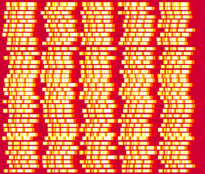
Figure 16: A simulated CCD frame as it will be produced by one of the four quadrants of the VIMOS spectrograph, showing 1/4 of the nearly 800 spectra that can be observed at once in the maximum multiplexing configuration.

6.3 X-ray Clusters as Tracers of High–z Structure

Given our still poor knowledge of galaxy formation and evolution, and on the contrary the relative simplicity of the physycs involved in the X-ray emission from clusters of galaxies, X-ray selected cluster have the potential to become one of the best tools for tracing large–scale structure at high redshifts [115]. The last few years have seen a number of studies on the evolution of the cluster abundance and of their X-ray luminosity function (e.g. [65]). These works have shown that the abundance of clusters with $L<10^{44}$ h^-2 erg s${}^{-1}\sim L^{*}$ does not seem to evolve significantly between the present epoch and $z\sim 1$. Although some uncertainties on how to relate this to the underlying evolution of the mass function still remain, these observations, together with the easiness in detecting X-ray clusters to high redshifts, qualifies them as excellent tracers for studying the evolution of large-scale structure.

The kind of flux limits that it is necessary to reach, to be able to detect at $z\sim 1$ objects with such luminosities, are comparable to the depth of ROSAT pointed observations, i.e. $\sim 10^{-14}\,erg\,s^{-1}\,cm^{-2}$. However, to be able to map large-scale structure at high redshifts, we shall need a survey covering an area significantly larger than the $\sim 100$ deg² typical of the serendipitous surveys constructed from the ROSAT PSPC archive, and in particular much less sparse than these. Such an X-ray survey has been recently proposed as the science drive for the construction of a wide-field X-ray satellite ([136]). Crucial for such a survey instrument is a novel design of the X-ray optics [137] which are able to obtain stable point–spread function of $\sim 10$ arcsec over a 1-degree diameter field, in contrast to the rapidly degrading resolution of classical Wolter–type telescopes [138]. A prototype of such innovative mirrors has been already constructed and successfully tested in the Merate labs of OAB. A more detailed discussion of the use of X-ray clusters as tracers of the evolution of structure, as a scientific case for future wide–angle deep X-ray surveys will be found in [115].

7 Conclusions

Looking at the various topics addressed in this paper, we can probably imagine the future development of this field during the first 10 years of the new Millennium as possibly moving along two directions.

One one side, the completion of the 2dF and in particular of the Sloan Digital Sky Survey will produce profound progress in the knowledge of many important statistical aspects of large–scale structure at $z\sim 0$. First of all, it is clear that something very interesting is hidden in the exact shape of the power spectrum near the expected turnover. While we seem finally to detect such turnover with some significance from the best samples now available, the data are still too poor on scales of $500-1000{\rm\mskip 5.0mu plus 5.0muh^{-1}\,Mpc}$ to sample it with sufficient resolution in $k$ space. This feature is more clearly detected when high–threshold objects as clusters of galaxies or Lyman–break galaxies are analysed. Larger samples of clusters of galaxies will be therefore essential: the REFLEX survey will be pushed down in flux by about a factor of two within the next two years, which will bring the number of clusters in the sample up to $\sim 800$, probing a volume extending to $z\sim 0.3$. At the same time, the sample of red luminous galaxies from the SDSS seems to represent the most promising data set for exploring the scales around the peak of $P(k)$ in sufficient detail. Also, the question on whether these features in the distribution of objects are partly a product of biasing, and therefore cannot be transferred to the matter power spectrum, will find an answer when detailed CMB anisotropy experiments will explore such scales. There seem to be all premises that the Planck Surveyor (see e.g. Efstathiou, these proceedings) will be able to provide this information to a high level of accuracy.

At the same time, 10–meter class telescopes equipped with a new generation of spectrographs give the opportunity to extend systematic studies of large samples of galaxies to redshifts above unity. I have briefly described the largest of these projects, the VLT–VIRMOS deep survey. Similar surveys with smaller sizes are being planned by different groups around the World, as newer instrumentation on very large telescopes commences operation. One example that I did not have time to discuss here is the Deimos spectrograph, under construction for the Keck II telescope [139].

The study of very large volumes of the Universe at high redshifts, however, will have to resort to using tracers which can be both more efficient and easier to understand than galaxies. X-ray selected clusters of galaxies provide this opportunity. Consequently, it would be highly significant if within the next $\sim 10$ years a large, possibly all–sky, survey in the X-ray band to a flux about 2 orders of magnitude fainter than the ROSAT All-Sky Survey ($\sim 10^{-14}$ erg s^-1 cm^-2) be performed. Concrete proposals in this direction have recently been presented [136], and will hopefully become reality in the near future.

References

References

- [1] Rood, H.J., 1998, ARA&A, 26, 245
- [2] Geller, M.J. & Huchra, J.P., 1989, Science, 246, 897
- [3] Giovanelli, R., & Haynes, M.P., 1991, ARA&A, 29, 499
- [4] Strauss, M.A., & Willick, J.A., 1995, Phys. Rep., 261, 271
- [5] Borgani, S., 1995, Phys. Rep., 251, 1
- [6] Guzzo, L., 1996, in Mapping, Measuring, and Modelling the Universe, P. Coles, V. Martinez & M.–J. Pons–Borderia eds., A.S.P. Conf. Ser. vol. 94, p. 157
- [7] Strauss, M.A., 1997, in Structure Formation in the Universe, A. Dekel & J.P. Ostriker eds. (astro-ph/9610033)
- [8] Chincarini, G., & Guzzo, L., 1998, in Proc. of V-eme Colloque de Cosmologie, H. De Vega ed., in press
- [9] da Costa, L.N., 1998, in Evolution of Large–Scale Structure: from Recombination to Garching, T. Banday & R. Sheth eds., in press (astro-ph/9812258)
- [10] Schuecker, P., Ott, H.-A., & Seitter, W.C., 1996, ApJ, 472, 485
- [11] De Lapparent, V., Geller, M.J., & Huchra, J.P., 1986, ApJ, 302, L1
- [12] Davis, M., Tonry, J., Huchra, J., & Latham, D. W. 1980, ApJ, 238, L113
- [13] Zwicky, F., Herzog, E., Wild, P., Karpowicz, M., & Kowal, C. 1961-68, Catalogue of Galaxies and of Clusters of Galaxies (Pasadena: California Institute of Technology)
- [14] Lauberts, A. 1982, The ESO/Uppsala Survey of the ESO(B) Atlas (München: European Southern Observatory)
- [15] Geller, M.J., et al., 1997, AJ, 114, 2205
- [16] Maddox, S.J., Efstathiou, G., Sutherland, W. J. & Loveday, J., 1990, MNRAS, 242, 43p
- [17] Heydon–Dumbleton, N.H., Collins, C.A., & MacGillivray, H.T., 1989, MNRAS 238, 379
- [18] Djorgowski, S.G., Gal, R.R., Odewahn, S.C., de Carvalho, R.R., Brunner, R., Longo, G., & Scaramella, R., 1998, in Wide Field Surveys in Cosmology, S. Colombi, Y. Mellier & B. Raban eds., (Paris: Edition Frontieres), p. 89
- [19] Collins, C.A., Nichol, R.C., & Lumsden, S.L., 1992, MNRAS, 254, 295
- [20] Davis, M., Efstathiou, G., Frenk, C. S., & White, S. D. M. 1985, ApJ, 292, 371
- [21] Loveday, J., Peterson, B.A., Efstathiou, G., & Maddox, S.J., 1992, ApJ, 390, 338
- [22] Parker, Q.A., & Watson, F.G., 1995, in Wide-Field Spectroscopy and the Distant Universe, S.J. Maddox and A. Aragón-Salamanca (eds.), World Scientific, Singapore, p. 33
- [23] Hill, J.M., 1988, in Fiber Optics in Astronomy, Samuel C. Barden ed., ASP Conference Series, Vol. 3, (San Francisco: ASP), p. 77
- [24] Avila, G., D’Odorico, S., Tarenghi, M., & Guzzo, L., 1989, The Messenger, 55, 62
- [25] Press, W.H., & Schechter, P., 1974, ApJ, 187, 425
- [26] Vettolani, G., Zucca, E., Zamorani, G., Cappi, A., Merighi, R., et al. (the ESP Team), 1997, A&A, 325, 954
- [27] Zucca, E., Zamorani, G., Vettolani, G., Cappi, A., Merighi, R., et al. (the ESP Team), 1997, A&A, 326, 477
- [28] Vettolani, G., Zucca, E., Merighi, R., Mignoli, D., Proust, D., et al. (the ESP Team), 1998, A&AS, 130, 323
- [29] Cappi, A., Zamorani, G., Zucca, E., Vettolani, G., Merighi, R., et al. (the ESP Team), 1998, A&A, 336, 445
- [30] Scaramella, R., Guzzo, L., Zamorani, G., Zucca, E., Balkowski, S., et al. (the ESP Team), 1998, A&A, 334, 404
- [31] Ramella, M., Zamorani, G., Zucca, E., Vettolani, G., Balkowski, C., et al. (the ESP Team), 1999, A&A, 342, 1
- [32] Guzzo, L., Bartlett, J., Cappi, A., Maurogordato, S., Zamorani, G., et al. (the ESP Team), 1999, A&A, in press (astro-ph/9901378)
- [33] Shectman, S.A., Landy, S.D., Oemler, A., Tucker, D.L., Lin, H., Kirshner, R.P., Schechter, P.L., 1996, ApJ, 470, 172
- [34] Lin, H., Kirshner, R.P., Shectman, S.A., Landy, S.D., Oemler, A., Tucker, D.L., Schechter, P.L., 1996, ApJ 464, 60
- [35] Taylor, K. 1995, in Wide-Field Spectroscopy and the Distant Universe, ed. S. J. Maddox and A. Aragón-Salamanca (Singapore: World Scientific), 15
- [36] Kaiser, N., 1986, MNRAS, 219, 785
- [37] Folkes, S.R., Ronen, S., Price, I., Lahav, O., Colless, M. et al. (the 2dF team), 1999, MNRAS, in press (astro-ph/9903456)
- [38] Colless, M., 1998, in Wide Field Surveys in Cosmology, S. Colombi, Y. Mellier & B. Raban eds., (Paris: Edition Frontieres), p. 77
- [39] Maddox, S.J., & 2dF Team, 1998, in Evolution of Large–Scale Structure: from Recombination to Garching, T. Banday & R. Sheth eds., in press
- [40] Fan, X., & SDSS Team, 1999, AJ, 118, 1
- [41] Loveday, J., 1999, in Second International Workshop on Dark Matter in Astro and Particle Physics, H.V. Klapdor-Kleingrothaus and L. Baudis eds, in press. (astro-ph/9810130)
- [42] Margon, B., 1998, Phil. Trans. R. Soc. Lond. A, in press (astro-ph/9805314)
- [43] Mandelbrot, B.B., 1982, The Fractal Geometry of Nature (San Francisco: Freeman)
- [44] Pietronero, L., 1987, Physica, 144A, 257
- [45] Guzzo, L., 1997, New Astronomy, 2, 517
- [46] Borgani, S., Martinez, V.J., Perez, M., & Valdarnini R., 1994, ApJ, 435, 37
- [47] Guzzo, L., Iovino, A., Chincarini, G., Giovanelli, R. & Haynes, M.P., 1991, ApJ, 382, L5
- [48] Martinez, V., 1999, Science, 284, 445
- [49] Padmanabhan, T., 1993, Structure Formation in the Universe (Cambridge: Cambridge University Press)
- [50] Coles, P., & Lucchin, F., 1995, The Origin and Evolution of Cosmic Structure (New York: John Wiley & Sons)
- [51] Peacock, J.A., 1999, Cosmological Physics (Cambridge: Cambridge University Press)
- [52] Saunders, W., et al., 1999, in Cosmic Flows Workshop, Victoria, July 1999, Courteau, S., Strauss, M., & Willick, J. eds., ASP Series, in press (astro-ph/9909190)
- [53] Jain, B., Seljak, U., & White, S.D.M., 1998, in Evolution of Large–Scale Structure: from Recombination to Garching, T. Banday & R. Sheth eds., in press (astro-ph/9901287)
- [54] Dekel, A., 1998, in Wide Field Surveys in Cosmology, S. Colombi, Y. Mellier & B. Raban eds., (Paris: Edition Frontieres), p. 47
- [55] Dressler, A., 1980, ApJ, 236, 351
- [56] Guzzo, L., Strauss, M.A., Fisher, K.B., Giovanelli, R., & Haynes, M.P., 1997, ApJ, 489, 37
- [57] Steidel, C., 1998, in Evolution of Large–Scale Structure: from Recombination to Garching, T. Banday & R. Sheth eds., in press (astro-ph/9811400)
- [58] Moscardini, L., Coles, P., Lucchin, F., & Matarrese, S., 1998, MNRAS, 299, 95
- [59] Tegmark, M., & Peebles, P.J.E., 1998, ApJ, 500, L79
- [60] Kaiser, N., 1984, ApJ, 284, L9
- [61] Postman, M., 1998, in Evolution of Large–Scale Structure: from Recombination to Garching, T. Banday & R. Sheth eds., in press (astro-ph/9810088)
- [62] Giacconi, R. & Gursky, H., 1974, X-ray Astronomy, (Dordrecht: Reidel Publishing Co.)
- [63] Henry, J.P., & Arnaud, K.A., 1991, ApJ, 372, 410
- [64] Henry, J.P., Gioia, I.M., Maccacaro, T., Morris, S.L., Stocke, J.T. & Wolter, A., 1992, ApJ, 386, 408
- [65] Rosati, P., 1998, in Wide Field Surveys in Cosmology, S. Colombi, Y. Mellier & B. Raban eds., Edition Frontieres, Paris, p. 219
- [66] Voges, W., Boller, T., Dennerl, K., et al., 1996, in Röntgenstrahlung from the Universe, H.U. Zimmermann, J.E. Trümper, H. Yorke (eds.), MPE Report No. 263, p. 637
- [67] De Grandi, S., Guzzo, L., Böhringer, H., Molendi, S., Chincarini, G., et al. (the REFLEX team), 1999, ApJ, 513, L17
- [68] Böhringer, H., 1994, in Studying the Universe with Clusters of Galaxies, H. Böhringer and S.C. Schindler (eds.), proc. of Ringberg workshop, MPE Report No. 256, p. 93
- [69] Romer, A.K., Collins, C.A., Böhringer, H., Cruddace, R.G., Ebeling, H., H.T. MacGillivray, & Voges, W., 1994, Nature, 372, 75
- [70] De Grandi, S., Böhringer, H., Guzzo, L., Molendi, S., Chincarini, G., et al. (the REFLEX team), 1999, ApJ, 514, 148
- [71] Böhringer, H., Guzzo, L., Collins, C.A., Neumann, D.M., Schindler, S., et al. (the REFLEX team), 1998, The Messenger, 94, 21
- [72] Peebles, P.J.E., 1980, The Large–Scale Structure of the Universe, (Princeton: Princeton University Press)
- [73] Groth, E.J. & Peebles, P.J.E., 1977, ApJ, 217, 385
- [74] Fisher, K.B., Davis, M., Strauss, M.A., Yahil, A., & Huchra, J.P. 1994, MNRAS, 267, 927
- [75] Ghigna, S., Bonometto, S., Guzzo, L., Giovanelli, R., Haynes, M.P., Klypin, A., & Primack, J.R., 1996, ApJ, 463, 395
- [76] Blumenthal, G. R., Faber, S. M., Primack, J.R., Rees, M.J., 1984, Nature, 311, 517
- [77] Guzzo, L., Bartlett, J., Cappi, A., Maurogordato, S., Zamorani, G., et al. (the ESP Team), 1998, in Evolution of Large–Scale Structure: from Recombination to Garching, T. Banday & R. Sheth eds., in press (astro-ph/9810173)
- [78] Tucker, D.L., Oemler, A., Kirshner, R.P., Lin, H., Shectman, S.A., et al., 1997, MNRAS, 285, L5
- [79] Loveday, J., Peterson, B.A., Efstathiou, G., Maddox, S.J., 1992b, ApJ, 390, 338
- [80] Ratcliffe, A., Shanks, T., Broadbent, A., Parker, Q.A., Watson, F.G., et al., 1996, MNRAS, 281, L47
- [81] Baugh, C.M., 1996, MNRAS, 280, 267
- [82] Kaiser, N., 1987, MNRAS, 227, 1
- [83] Dekel, A., & Aarseth, S.J., 1984, ApJ, 283, 1
- [84] Branchini, E., Guzzo, L., & Valdarnini, R., 1994, ApJ, 424, L5
- [85] Baugh, C.M., & Efstathiou, G.P., 1993, MNRAS, 265, 145
- [86] Bahcall, N.A. & Soneira, R., 1983, ApJ, 270, 20
- [87] Collins. C.A., Guzzo, L., Nichol, R.C., & Lumsden, S.L., 1995, MNRAS, 274, 1071
- [88] Postman, M., Huchra, J., & Geller, M.J., 1992, ApJ, 384, 404
- [89] Dalton, G.B., Maddox, S.J., Sutherland, W.J., & Efstathiou, G., 1997, MNRAS, 289, 263
- [90] Borgani, S., Plionis, M., & Kolokotronis, V., 1999, MNRAS, 305, 866
- [91] Guzzo, L., Böhringer, H., Schuecker, P., Collins, C.A., Schindler, S., et al (the REFLEX Team), 1999, The Messenger, 95, 27
- [92] Collins, C.A., & the REFLEX Team, in preparation
- [93] Mo, H.J., & White, S.D.M., 1996, MNRAS, 282, 347
- [94] Bertschinger, E., 1992, in New Insights into the Universe, V.J. Martinez, M. Portilla, D. Saez eds., (Berlin: Springer-Verlag), p. 65
- [95] Fisher, K.B., Davis, M., Strauss, M.A., Yahil, A., & Huchra, J.P. 1994a, MNRAS, 266, 50
- [96] Fisher, K. B., Davis, M., Strauss, M. A., Yahil, A., & Huchra, J. P. 1993, ApJ, 402, 42
- [97] Feldman, H., Kaiser, N., & Peacock, J. 1994, ApJ, 426, 23
- [98] Tadros, H. & Efstathiou, G. 1995, MNRAS, 276, L45
- [99] da Costa, L.N., Vogeley, M.S., Geller, M.J., Huchra, J.P., & Park, C. 1994b, ApJ, 437, L1
- [100] Tadros, H., & Efstathiou, G.P., 1996, MNRAS, 282, 138
- [101] Hoyle, F., Baugh, C.M., Ratcliffe, A., & Shanks, T., 1999, MNRAS, 309, 659
- [102] Tegmark, M., Hamilton, A.J.S., Strauss, M.A., Vogeley, M.S., & Szalay, A.S., 1998, ApJ, 499, 555
- [103] Vogeley, M.S., & Szalay, A.S. 1996, ApJ, 465, 34
- [104] Sutherland, W., Tadros, H., Efstathiou, G., Frenk, C.S., Keeble, O., et al., 1999, MNRAS, in press (astro-ph/9901189)
- [105] Schuecker, P., & the REFLEX Team, in preparation
- [106] Carretti, E., Bertoni, C., Messina, A., Zucca, E., & Guzzo, L., 1999, MNRAS, submitted
- [107] Lin, H., Kirshner, R.P., Shectman, S.A., Landy, S.D., Oemler, A., Tucker, D.L., & Schechter, P.L., 1996, ApJ, 471, 617
- [108] Peacock, J.A., 1997, MNRAS, 284, 885
- [109] Hamilton, A.J.S., Kumar, P., Lu, E., & Matthews, A., 1991, ApJ, 374, L1
- [110] Saunders, W., Rowan-Robinson, M., & Lawrence, A., 1992, MNRAS, 258, 134
- [111] Retzlaff, J., Borgani, S., Gottlober, S., Klypin, A., & Müller, V., 1998, NA, 3, 631
- [112] Tadros, H., Efstathiou, G., & Dalton, G., 1998, MNRAS, 296, 995
- [113] Guzzo, L., 1999, //http://www.mso.anu.edu.au/DunkIsland/Proceedings/Guzzo/
- [114] Einasto,J., Einasto, M., Gottloeber, S., Mueller, V., Saar, V., et al., 1997, Nature, 385, 139
- [115] Borgani, S., & Guzzo, L., in preparation
- [116] Landy, D.S., Shectman, S.A., Lin, H., Kirshner, R.P., Oemler, A.A., & Tucker, D. 1996, ApJ, 456, L1
- [117] Broadhurst, T.J., Ellis, R.S., Koo, D.C., & Szalay, A.S., 1990, Nature, 343, 726
- [118] Kaiser, N., & Peacock, J.A., ApJ, 379, 482
- [119] Guzzo, L., Collins, C.A., Nichol, R.C., & Lumsden, S.L., 1992, ApJ, 393, L5
- [120] Ettori, S., Guzzo, L., & Tarenghi, M., 1997, MNRAS, 285, 218
- [121] Broadhurst, T.J., Szalay, A.S., Koo, D.C., Ellman, N., Ellis, R.S., et al., in preparation
- [122] van de Weygaert, R., 1991, MNRAS, 249, 159
- [123] Bardeen, J., Bond, J. R., Kaiser, N., & Szalay, A., 1986, ApJ, 304, 15
- [124] Einasto, J., Einasto, M., Frisch, P., Gottloeber, S., Mueller, V., et al., 1997, MNRAS, 289, 813
- [125] Broadhurst, T.J., & Jaffe, A.H., 1999, ApJ, submitted (astro-ph/9904348)
- [126] Eisenstein, D.J., Hu, W., Silk, J., & Szalay, A.S., 1998, ApJ, 494, L1
- [127] Meiksin, A., White, M., & Peacock, J.A., 1999, MNRAS, 304, 851
- [128] Silk, J., & Gawiser, E., 1998, in Proc. of Nobel Symposium - Particle Physics and the Universe, Physica Scripta, in press (astro-ph/9812200)
- [129] Baugh, C.M., Cole, S., Frenk, C.S., Lacey, C.G., 1998, ApJ, 498, 504
- [130] Somerville, R.S., & Primack, J.R., 1999, MNRAS, in press (astro-ph/9802268)
- [131] Governato, F., Baugh, C.M., Frenk, C.S., Cole, S., Lacey, C.G., et al., 1998, Nature, 392, 359
- [132] Iovino, A., Warren, S.J., Hewett, P., & Shaver, P.A., 1997, Astroph. Lett. & Comm., 36, 327.
- [133] Lilly, S.J., Le Fèvre, O., Crampton, D., Hammer, F., & Tresse, L., 1995, ApJ, 455, 50
- [134] Le Fèvre, O., Vettolani, P. Maccagni, D., Mancini, D., Picat, J.P., et al. (the VIRMOS Consortium), 1998, in Wide Field Surveys in Cosmology, S. Colombi, Y. Mellier & B. Raban eds., (Paris: Edition Frontieres), p. 327
- [135] Borgani, S., Rosati, P., Tozzi, P., & Norman, C., 1999, ApJ, 517, 40
- [136] Chincarini, G., 1999, in Observational Cosmology: the Development of Galaxy Systems (Sesto Workshop 1998), in press. (astro-ph/9902184)
- [137] Burrows C.J., Burg R., & Giacconi R., 1992, ApJ, 392, 760
- [138] Citterio, O., Campana, S., Conconi, P., Ghigo, M., Mazzoleni, F., et al., 1999, in Proc. of 1999 SPIE Meeting, in press
- [139] Davis., M. & Faber, S.M., 1998, in Wide Field Surveys in Cosmology, S. Colombi, Y. Mellier & B. Raban eds., (Paris: Edition Frontieres), p. 333