On the Reliability of Cross Correlation Function Lag Determinations in Active Galactic Nuclei
Abstract
Many AGN exhibit a highly variable luminosity. Some AGN also show a pronounced time delay between variations seen in their optical continuum and in their emission lines. In effect, the emission lines are light echoes of the continuum. This light travel–time delay provides a characteristic radius of the region producing the emission lines. The cross correlation function (CCF) is the standard tool used to measure the time lag between the continuum and line variations. For the few well–sampled AGN, the lag is 1–100 days, depending upon which line is used and the luminosity of the AGN. In the best sampled AGN, NGC 5548, the H lag shows year–to–year changes, ranging from 8.7 days to 22.9 days over a span of 8 years. In this paper it is demonstrated that, in the context of AGN variability studies, the lag estimate using the CCF is biased too low and subject to a large variance. Thus the year–to–year changes of the measured lag in NGC 5548 do not necessarily imply changes in the AGN structure. The bias and large variance are consequences of finite duration sampling and the dominance of long timescale trends in the light curves, not due to noise or irregular sampling. Lag estimates can be substantially improved by removing low frequency power from the light curves prior to computing the CCF.
1 Introduction
Active galactic nuclei (AGN) often exhibit variable luminosity. In several highly variable AGN, the observed UV/optical emission–line fluxes are well correlated with the continuum variations, but with a time delay (e.g. Peterson 1988; Ulrich, Maraschi & Urry 1997). In effect, the line emission is a light echo of the photoionizing continuum. For Seyfert 1 galaxies, the well–measured time delays (“lags”) range from 1–80 d, and depend on which emission line is observed (the higher ionization lines respond more quickly to continuum variations than do lower ionization lines; see e.g. Clavel et al. 1991; Peterson et al. 1998b). The observed time delay gives a characteristic timescale that, under reasonable assumptions (i.e. the lines are responding to photoionization, the observed continuum closely mimics the photoionizing continuum, and the light–travel timescale is the most relevant timescale), provides a characteristic lengthscale (see e.g. Peterson 1988, 1993). Thus the observed lag between AGN continuum and emission–line light curves gives a measure of the size of the line–producing region, i.e., the broad–line region (BLR). Note that these lengthscales correspond to angular scales of microarcseconds on the sky, so “echo mapping” studies offer the potential for extremely high spatial resolution studies of AGN (e.g. the proceedings by Peterson and by Horne in Gondhalekar, Horne & Peterson 1994).
The Seyfert galaxy NGC 5548 has been the target of several variability studies and has been intensely monitored for several years (e.g. Peterson et al. 1999). Of particular interest are the time lag determinations for the H emission line with respect to the optical continuum. The lag (as defined by the peak of the cross correlation function) ranges from 8.7 d to 22.9 d over a span of 8 years (1989-1996) with an rms scatter of 4.5 d (Peterson et al. 1999). These variations have been interpreted as evidence for real structural changes in the BLR, either due to physical changes of the ensemble of BLR clouds or to changes in the photoionizing radiation field (e.g. Wanders & Peterson 1996). The dynamical timescale for the BLR () is on the order of a few years, so changes in the BLR structure on this timescale is a realistic possibility.
However, there is considerable difficulty in determining the lag from AGN time series, in particular, because (i) the data are short in duration compared to the timescales of interest and (ii) the data are usually not equally sampled. Previous studies have investigated the issue of noisy and poorly sampled data, e.g., see the summary in Koen (1994). Several different methods for computing the CCF have been constructed: the interpolated CCF (“ICCF” — e.g. Gaskell & Peterson 1987); the discrete CCF method (“DCF” — Edelson & Krolik 1988); the inverse Fourier transform of the discrete power spectrum (Scargle 1989); and the Z–transform CCF (Alexander 1997). In addition, methods other than the CCF have been used to measure time lags, e.g., optimal reconstruction via minimizing (Press, Rybicki & Hewitt 1992) or a parametric approach (i.e., modeling the light curves as random walks; Koen 1994). For comparisons of the DCF and ICCF methods, see e.g., Litchfield, Robson & Hughes (1995), White & Peterson (1994), and Rodriguez–Pascual, Santos–Lleo & Clavel (1989). Simulations have shown that these methods can provide reasonably accurate determinations of the lag under sampling and noise conditions similar to the actual observations (e.g. Peterson et al. 1998a; White & Peterson 1994, Koratkar & Gaskell 1991b). Hence the changing H lag in NGC 5548 seems quite real.
In this paper we consider two additional sources of “error” in the CCF lag determinations, which to our knowledge have not been fully addressed in the astronomical literature. The first is a bias inherent in the definition of the CCF such that, on average, the computed CCF lag is not the true lag. The second error is concerned with gross changes in the CCF due to changes in the ACF of the continuum. These changes in the ACF are not real, in that the underlying physical process generating the continuum variations have not changed; they are simply statistical fluctuations inherent in any finite realization of a stochastic process.
In §2 we define the autocorrelation function (ACF), cross correlation function (CCF) and transfer function and examine the relationships between them in the AGN echo mapping context. Several aspects of the CCF are examined in §3, and at the risk of being overly pedagogical, we present this material in detail because they are crucial to the interpretation and usefulness of the CCF. In particular, the bias inherent in the definition of the CCF and the error in the lag determination are highlighted. To illustrate and quantify these “problems” with the CCF, simulations tailored to match the characteristics of the H observations of NGC 5548 are presented in §4. The simulations clearly show the bias and large variance present in the CCF. Additional simulations are also presented to: (1) explore a wider range in parameter space, (2) help quantify the amount of bias and variance, and (3) illustrate how the bias and variance can be reduced by removing low frequency trends from the light curves. We conclude with a discussion of our results in §5.
2 The ACF, CCF and Transfer Function
2.1 The Standard Definitions of the ACF and CCF
The auto– and cross–correlation functions are standard tools of time series analysis (e.g. Jenkins & Watts 1969; Box, Jenkins & Reinsel 1994; Chatfield 1996; Wall 1996). The cross–correlation function, sometime called the serial correlation function, quantifies the amount of similarity or correlation between two time series as a function of the time shift (i.e., the delay or “lag”) between the two time series. The auto–correlation function (ACF) measures the similarity of a single time series to a delayed version of itself.
The standard definition of the cross–correlation function of two time series and sampled at discrete times () with equal sampling () is:
| (1) |
where the lag is the size of the time shift: , and , are the means of and (see e.g. Jenkins & Watt (1969), Chatfield (1996)). The ACF is similarly defined, with itself in place of . [NB: for negative lags, simply interchange and .]
It will be helpful to express the CCF more succinctly, and we will use the continuous definition to do so:
| (2) | |||
| (3) |
It should be explicitly stated that we use equations (2) & (3) only as shorthand representations of equation (1), as the discrete and continuous CCF are not the same. Also note that in this nomenclature and are by definition zero and the light curves have been normalized to unity variance.
2.2 The transfer function
AGN broad emission–line light curves are not simply delayed copies of the continuum light curves. This can be understood as a geometrical effect, as first pointed out by Blandford & McKee (1982): the line–emitting region extends over a large volume of space, so the light travel time across the BLR is significant. The integrated line light curve thus appears as a delayed and blurred version of the continuum light curve.
Blandford & McKee (1982) expressed the relationship between the line emission and the continuum emission as:
| (4) |
The geometry and responsivity of the gas is contained in the “transfer function” , and equation (4) simply states that the line light curve is equal to the continuum light curve convolved with the transfer function. The transfer function can be thought of as a “point spread function”, “impulse–response function”, or as a filter of a linear moving average process with the continuum as the driver (but note that in this interpretation the continuum is not an uncorrelated white noise process). Only if is a delta function will the be an identical (but lagged) version of [NB: we use the term “identical” loosely here: we mean is identical to within a scale factor and constant, allowing for and a background contribution to both the line and continuum. We also implicitly assume , i.e., is purely causal.] Recovering the transfer function is a major goal of variability studies in AGN, as it contains information on the geometry and kinematics of the BLR. The reader is referred to Horne (1994), Pijpers & Wanders (1994), Krolik & Done (1995), Vio, Horne & Wamsteker (1994), and the proceedings in Gondhalekar, Horne & Peterson (1994) for a discussion of the transfer function and inverting equation (4) to solve for .
2.3 The relationship between the ACF, CCF and transfer function
From the definitions it can be shown (e.g. Koratkar & Gaskell 1991a; Penston 1991; Sparke 1993) that
| (5) |
i.e., the cross–correlation function is equal to the transfer function convolved with the auto–correlation function of the continuum. In this representation it becomes clear that the theoretical CCF is identical to a blurred version of the transfer function.
If the continuum light curve consists of a well–isolated sharp pulse, or equivalently, its power spectrum is white, then its ACFc is a delta function and the CCF is then identical to . In this circumstance the peak of the CCF will occur at the same lag as the peak of . More generally, the ACF is a broad and even function, so the peak of the CCF will not necessarily occur at the same lag as the peak in . The lag determined from the CCF should be considered only a characteristic time scale.
Equation (5) concisely describes the fundamental issue we address in this paper: the determination of the lag between line and continuum light curves depends on both the shape of the transfer function and the ACF of the continuum. However, it is crucial to understand that eq. (5) is valid only in the infinite duration limit — for finite limits, it is straightforward to show the equality is not true.
3 Practical Issues
Just as with Fourier analysis, the difference between the mathematical CCF and the experimental (discrete and finite–sampled) CCF can be large. Thus it is useful to examine some of the details and practical issues concerning the computation of the CCF, with emphasis on the AGN echo mapping problem. Several of the issues discussed in this section will be illustrated with simulations presented in §4. Problems concerning unequal sampling have been discussed in the literature (see the references in the introduction) and will not be repeated here.
3.1 General aspects of the CCF
3.1.1 “self correlation”
The individual points in the ACF and CCF are highly correlated with themselves, i.e., neighboring points are not independent (a derivation can be found in Jenkins & Watts (1969)). In general, the neighboring values in the ACF/CCF are more correlated with themselves than neighboring values in the original time series (Jenkins & Watts 1969). It is important to be aware of this “self–correlation” in the interpretation of the ACF/CCF because trends in the ACF/CCF are long–lived, e.g. it can take a surprisingly long time for the ACF/CCF to decay from a peak. This can also lead to spurious large values of the CCF, especially for time series whose ACFs contain intrinsically broad peaks — see e.g. Figs. 1–4 in Koen (1994).
3.1.2 bias
The CCF as defined in equation (1) has the peculiar property that the summation in the numerator goes from to , but the normalization is , not . This normalization is chosen primarily because the variance of the CCF is then reduced, i.e., the sample CCF is a better estimator of the true CCF in the mean square error sense when the normalization is used (Jenkins & Watts 1969). This normalization also guarantees that the CCF is always bounded by , and the autocorrelation matrix is positive semi–definite so that the ACF and power spectrum are Fourier transform pairs — the Wiener–Khinchin theorem (e.g. Jenkins & Watt 1969). However, the normalization means that eq. (1) is only an asymptotically unbiased estimator of the correlation function, and its use introduces a well–known bias towards zero (e.g. Kendall 1954; Marriott & Pope 1954; Otnes & Enochson 1978; Chatfield 1996). This bias grows worse with increasing lag, and results in a triangular–shaped reduction of the CCF and hence underestimates the lag of the peak of the CCF. The trade–off between the bias and variance in an estimator is a common problem in statistics: often one must choose between precision (low variance) and accuracy (low bias). For the CCF, the bias goes as while the variance goes as ; this is why reducing the bias has not been treated with equal importance as reducing the variance (Tjostheim & Paulsen 1983). It is argued that in most cases and , so one can tolerate a small bias to achieve a large the reduction in variance. Furthermore, eq. (1) is extremely simple to compute. For these reasons the normalization has gained predominance.
In the case of AGN variability, however, the ACFs are intrinsically broad and the lags of interest are usually a substantial fraction of the duration of the observations, hence this bias can lead to a significant underestimation of the lag. As Scargle (1989) points out, this bias can be devastating. One could simply replace the term with , but then the CCF has the very undesirable property that it can exceed unity. Indeed, it is likely to exceed unity because of the self–correlation in the CCF; the ACF at =0 is forced by definition to be exactly 1, so due to self–correlation the value of the AGN ACF at =1 will tend to be close to 1 as well, and so on for many lags. As shown by Marriott & Pope (1954) and by Kendall (1954), the bias in the estimated ACF at lag depends, in general, on the value on the true ACF at lags and earlier, a consequence of the strong self–correlation. Because of this, the bias cannot be removed a priori and the simple attempt at bias correction will in general fail.
In his method for coping with unequally sampled data, Scargle (1989) suggests renormalizing the ACF with the ACF of the sampling pattern, which will remove both the effects of this bias as well as the effects of irregular sampling. Scargle notes that this correction is on average equivalent to replacing term with , and so it also allows values of the CCF to exceed unity.
We find that in practice, the normalization has the side–effect of boosting noise at large lags, but even worse, the shape of the ACF can be modified, and peaks in the CCF at can be shifted to longer lags. This is totally unacceptable for our purposes and so this proposed renormalization is rejected.
To the best of our knowledge, most of the effort in reducing the bias in the CCF as given in equation (1) has been motivated by the desire to accurately determine the Yule–Walker filter coefficients of a stochastic moving average (or autoregressive) process. These filter coefficients can be determined from the ACF, and in particular, the first few lags of the ACF. Since this usually corresponds to , a “better” definition of the ACF has not been sought and instead bias–corrections have been developed to treat the specific problem of determining the filter coefficients (e.g. Kendall 1954; Tjostheim & Paulsen 1983; Marriott & Pope 1954). In their noteworthy analysis, Sutherland, Weisskopf & Kahn (1978) address the question of bias specifically for the ACF in the case of a noisy and finite length shot–noise light curve, and in particular, they derive a “partially unbiased” definition for the ACF. They show that in addition to the bias that is present in the noise–free case, there is an additional reduction of the ACF due to noise; this comes about because the normalization of the ACF depends on the variance of the light curve, and in the presence of noise, the variance itself is biased too high. Thus the value of CCF depends on the signal–to–noise ratio (S/N) of the data. The motivation for their work was to deduce the correlation time constant for the shot noise in Cyg X-1. They show that this can be deduced in an unbiased fashion from the ratio of the ACF at lags =1 and =2. It is not obvious that their partially unbiased ACF, suitable for small lags, is applicable to the CCF at large lags but this is a topic worth pursuing.
Another possible method to reduce the bias in the ACF is to use the “jackknife” or Quenouille method (see e.g. Chatfield 1996): , where is the ACF of the first half of the data set and is the ACF of the latter half. The bias in is reduced from order to . Although this reduces the length of the already too short AGN time series by a factor of two, it does allow one to check the stationarity assumption between the two halves. While we have not investigated this bias correction method, it is worth consideration in future studies.
3.1.3 peak or centroid?
The peak of the CCF gives the lag where the two time series are most highly linearly correlated. Yet the peak of the CCF need not correspond to the peak of the transfer function — indeed, the transfer function may not have a well–defined peak at all. The peak of the AGN line–continuum CCF tends to correspond to where the line echo response is most coherent, i.e. the innermost region of the BLR, and hence can underestimate the BLR size (e.g. Gaskell & Sparke 1986; Edelson & Krolik 1988; Robinson & Perez 1990; and especially Pérez et al. 1992).
To avoid the uncertainty in the interpretation of the peak of the CCF, the centroid (center of gravity) of the CCF is often quoted. In the infinite duration limit, the centroid of the CCF corresponds to the centroid of (e.g. Penston 1991; Koratkar & Gaskell 1991a111The end result is correct, but the derivation contains an error.). As Penston points out, this is intuitively obvious because the ACF is an even function and the CCF is the convolution of and the ACF. The lag determined from the centroid of the CCF is therefore sometimes preferred over the peak lag (e.g. Peterson et al. 1998a) because it is more easily interpreted as the responsivity–weighted radius of the BLR. Thus it has become common practice to quote both the peak and centroid of the CCF when making lag estimations.
However, the centroid suffers from three serious flaws. First, the centroid of the CCF based on finite–duration light curves is not identically the centroid of . This follows directly from the fact that the sample CCF is not identically the sample ACF convolved with , i.e., eq. (5) is only true in the infinite duration case. The best that can be hoped for is that the centroid of the CCF is approximately the same as the centroid of if the durations of the light curves are much longer then the lag. Second, the centroid is poorly defined. Obviously not all points in the CCF should be used to define the centroid, only those near the peak should be included. So some threshold is arbitrarily set, and the value of the centroid can depend very strongly on what threshold is chosen (see Koratkar & Gaskell 1991a,b). Third, because the centroid integrates over a range of values of the CCF, it is more sensitive to the bias inherent in the CCF than the peak. Thus the centroid underestimates the lag more than the peak. This bias in the centroid then negates the argument that the centroid gives a more characteristic BLR size than the peak. The problems with using the centroid to estimate the lag will be illustrated via the simulations in §4, where it will be seen that the centroid of the CCF generally fares worse than the peak (see also Pérez et al. 1992). 222 A similar preference for the use of the CCF peak has been previously shown by Wade & Horne (1998). In using spectroscopy to measure radial velocities, they found that fitting a very narrow Gaussian to the peak of the CCF gives a more reliable velocity estimate than fitting a broad Gaussian to the CCF.
3.1.4 the removal of the mean
The terms and in eq. (1) are the mean values of the entire light curves. For a stationary process, the sample mean of all the data is clearly the best estimate for the mean. But for a finite duration realization of a stochastic process, this may not be the case. Scargle (1989) makes the point that for positive definite quantities (e.g. fluxes), removing the sample mean is not always desirable. Instead, removing a fraction of the mean may provide a better CCF estimate. The question of what fraction to use depends upon the data themselves, and experimentation (and judgment) is required to find what fraction is optimal. One could in fact solve for the mean as a free parameter (e.g. Press, Rybicki & Hewitt 1992).
The standard definition of the CCF (eq. (1)) implicitly assumes the time series are stationary in their mean and variance. To help fulfill this requirement, one can “pre–whiten” the data by: (a) removing a linear (or higher order) fit, or (b) apply a differencing operator to the data. In the latter case, the data to be analyzed are derived from differences of successive pairs of the light curve: . The differencing operator is in fact a high–pass filter, and under high signal–to–noise ratio (S/N) conditions it is the preferred technique to remove trends — see e.g. Koen (1993, 1994). Unfortunately, it fails in practice because the S/N of currently available UV/optical AGN variability data is too low, and one is left mostly with noise.
3.1.5 the “local” CCF
An alternative definition of the CCF in which only those points that overlap at a given lag () are used to determine the mean and standard deviations is:
| (6) |
where and are the means of and in the overlap interval. We refer to this method of computing the CCF as the “local CCF” method. The local CCF naturally accounts for the versus problem because only those values of the light curves which overlap at a lag are included in the determination of the mean and standard deviations. The value of the CCF determined in this fashion is then identical to the product–moment correlation coefficient, also known as Pearson’s statistic (see e.g. Press et al. 1996 for a discussion) and this is the method used by White & Peterson (1994). The simulations in §4 will demonstrate that while the bias is not completely removed, this definition produces a CCF with far more desirable qualities. Notice that in effect the local CCF method applies a varying high–pass filter to the data whose cutoff frequency depends on the number of points in the time series at a particular lag (i.e. ). Thus the local CCF handles data containing low frequency trends far better than the standard CCF. For these reasons we prefer the local CCF over the standard definition (eq. (1)), but we caution that CCFs constructed in this manner are for lag determinations only, as to our knowledge the statistical properties and the relationship between the local CCF and the (a) inverse Fourier transform of the power spectrum or (b) coefficients of autoregressive (or moving average) processes has not been investigated. Jenkins & Watts (1969) do not recommend the local CCF for these reasons; however, recovery of ARMA coefficients and the power spectrum is not the goal of CCF analysis in the context of AGN echo studies — the determination of an unbiased lag estimate is.
3.1.6 the CCF: an intuitive statistic?
As Jenkins & Watts (1969) point out, it should be kept in mind that the standard CCF as defined by eq. (1) has not in any way been proven to be the best possible estimator. It is used primarily because it is an efficient, consistent estimator with intuitive appeal. However, our intuition can be grossly incorrect in cases when is not . So we should not consider equation (1) to be sacrosanct, and in particular, the “local ccf” implementation largely reduces the bias problems mentioned above, and in our simulations, yielded results more akin to our expectations than the standard method.
The local CCF has an easy to understand interpretation (see e.g. Bevington & Robinson 1992): For a given lag , there are overlapping points. A least–squares straight–line fit to the mean–subtracted values of versus will yield some slope . A non–zero slope suggests a correlation. However, the value of cannot be used as a measure of the strength of the correlation because and could be strongly correlated and yet have a small slope (e.g., if spanned many orders of magnitude more than the slope would be small even if there were a perfect correlation). Reversing the dependent and independent variables and fitting a line to versus will give a slope . As with , a non–zero slope implies a possible correlation. The product is then a measure of the correlation strength, independent of the slope of the relationship. The quantity = local CCF().
Despite the apparent intuitive appeal of using the CCF to detect a correlation, a few caveats and comments are in order: (i) equation (1) defines a linear correlation coefficient between two series. The restriction to a linear correlation is arbitrary, and a non–linear analysis may prove fruitful; (ii) the use of non–parametric correlation tests (such as Spearman’s rank–order correlation) may be of value (see Press et al. 1996) since they tend to be more robust; (iii) our intuition is based on the abstract mathematical case of infinite duration time series, and this can be grossly misleading.
3.1.7 finite duration sampling
Flagrant violations of our intuition about the ACF/CCF can occur if the duration of the light curves are finite. The problem is particularly serious in the AGN context because the lags of interest are often a sizeable fraction of the total duration of the light curves.
In theory, the CCF should be the convolution of the ACF and the transfer function . But even in the absence of noise and with ideal sampling this will often not even be approximately true. Leaving aside the effects of bias in the standard CCF definition, the major cause of the difference between the expected and measured CCF is due to changes in the observed ACF. For any finite realizations of a stochastic process, the ACFs will not be exactly the same, even if the underlying generating process is unchanged. The usual interpretation of the CCF demands stationarity in the mean and variance, but this is in general unlikely for finite duration observations generated from a stochastic process, and in particular, AGN light curves have red power spectra and are far from being stationary on year–to–year timescales. As a consequence, the ACFs can vary from epoch to epoch, and with it the CCF lags, despite no real physical changes in the emission producing mechanism (either the continuum source or BLR). To help mitigate this effect, low frequency power in the data should be removed, or if the data S/N allow, a differencing operator should be applied. In §4.2 simulations will show the improvements in the CCF lag determination that can result by removing low–frequency trends and softening the edge effects in the finite light curves.
3.2 The errors in the lag determination
Real data have finite time resolution, contain noise, may be unequally sampled, and have finite duration. The effects of finite sampling rate are not a problem provided the data are not undersampled, and the effects of noise and unequal sampling have been discussed extensively in the astronomical literature, e.g., White & Peterson (1994), Maoz & Netzer (1989), Peterson et al. (1998a), and references therein. Simulations have shown that the CCF can be satisfactorally recovered under a wide range of realistic sampling and noise conditions. However, the effects of bias and finite duration observations have not be properly appreciated when considering the errors in the lag determination.
Ignoring bias for the moment, there are two distinct sources of error: (i) external errors due to observational noise and irregular sampling, and (ii) internal errors due to the random nature of the light curves. Finite duration sampling of the light curves brings about the latter source of error. It is independent of observational noise or the sampling pattern.
Maoz & Netzer (1989) estimated the errors on the CCF by producing a set of simulated line and continuum light curves with random sampling and noise, then constructed a “cross–correlation peak distribution” (CCPD) histogram showing the spread in lags of the peak. From the CCPD one can measure the mean (or median or mode) and the associated uncertainty on the lag for the chosen model. For their continuum time series they used either an interpolated version of the Peterson et. al. (1985) Akn 120 light curve or the Clavel et al. (1987) NGC 4151 light curve. So in fact identical parent continuum light curves were used for each of their two sets of simulations. The CCPD clearly shows a large spread in the determinations of the lag, but this spread only shows the effects of the sampling and observational noise.
The White & Peterson (1994) analysis is more general in that the continuum light curves are not identical; instead they have a power–law power density spectrum (PDS) of either or , motivated by the power spectra of NGC 5548 (Clavel et al. 1991) and NGC 3783 (Reichert et al. 1994), respectively. However, although the continuum light curves are different in each realization, they all have very similar ACFs (since by definition they have identical PDS and the Weiner–Khinchin theorem states that the PDS and ACF are Fourier pairs). The scatter in their CCPD is therefore dominated by observational noise and irregular and sparse sampling, and do not realistically include finite sampling–induced changes in the ACF.333Technical note: The construction scheme used by White & Peterson (1994) to add backgrounds to the light curves (such that the fractional rms “” matches the observed value of 0.32 for NGC 5548) results in a correlation between the intrinsic rms of the light curve and the amount of observational noise added. The simulated noise is therefore not constant, nor is it dependent only on the simulated fluxes; it also depends on the amount of intrinsic variability. This correlation may result in a slight overestimate of the reliability of the lag determinations, since for continuum light curves with small intrinsic fluctuations the observational noise is reduced.
In their pioneering work, Gaskell & Peterson (1987) do indeed take into consideration the changes in the ACF, since their simulated continuum light curves were generated using a first–order autoregressive model (e.g. see Jenkins & Watts 1969). In fact their figure 12 shows the problems mentioned in the previous section: bias in the correlation coefficient (height of the peak of the CCF) and bias in the position of the peak of the CCF (towards too small lags). However, the emphasis of their work was to highlight their interpolation method for coping with irregular, sparse sampling and observational noise, and neglected the issues we investigate here.
The more recent analysis of CCF uncertainties by Peterson et al. (1998a) attempts to generate a realistic CCPD using a combined Monte Carlo and bootstrap method (see e.g. Press et al. 1996 for a discussion of the bootstrap method). The Monte Carlo “flux randomization” jitters the observed data values by a random amount consistent with the observational noise, while the bootstrap “random subset selection” picks subsets of the time series at random. The authors conclude that the method produces estimates of the errors that are generous, i.e., slightly larger than the errors in the parent distribution. While their detection of a wavelength–dependent lag in NGC 7469 seems irrefutable, the analysis of the errors is only partially complete. In their simulations, the method used to generate the light curves was nearly identical to that in White & Peterson (1994), so they do not precisely mimic reality in the construction of the parent CCPD distribution. The fact that the CCPD generated via a Monte Carlo and bootstrap treatment of a single light curve realization is larger than the parent CCPD is comforting, but this may still underestimate the true uncertainty in the lag.
Note that the Peterson et al. (1998a) implementation of the bootstrap omits roughly 37% of the observed continuum and line data pairs; this can be avoided if one reverses the order of the Monte Carlo flux and the bootstrap sampling. By bootstrap sampling first, one can keep track of the data pairs that are selected more than once and the error bars on those points can be reduced accordingly, before the data are jittered by the Monte Carlo method. This brings the method more in line with the standard bootstrap technique (Efron 1983; Diaconis & Efron 1983), where in essence the data are not omitted, but rather, a random weighting is given to the points — in the analysis, a weight of zero is assigned to a datum if it is not chosen, and a weight of is assigned if that datum is selected times. The process is repeated many times and in all cases the total number of input values used is constant. Note that for data whose error bars are roughly constant, it is the bootstrapping, not the Monte Carlo step, that gives the correct error distribution, and for this reason the modification of the Peterson et al. (1998a) technique is important. For the equal sampling case with equal size error bars, Monte Carlo flux randomization alone can grossly underestimate the CCPD width.
The Monte Carlo plus bootstrap method as suggested by Peterson et al. (1998a) and modified to improve efficiency as stated above appears to be the best way to estimate the CCPD and hence the uncertainty of the lag for a given time series. Yet if the continuum light curve is not at least weakly stationary, knowing the uncertainty for a given realization does not give a reliable estimate for the full range of scatter in the determination of the lag. Even if the continuum generating process is stationary on long timescales, short observations may mimic non–stationarity. The fact that the observed yearly mean fluxes from NGC 5548 are not consistent with each other is evidence that the process is not stationary over the timescales of interest and so comparison of CCF from different years is problematic. Only if the ACFs from year to year are identical can the changes in the lag be ascribed to changes in the transfer function and hence changes in the BLR. In summary, even if large and apparently significant changes in the lag are observed, these do not necessarily imply changes in the AGN/BLR — the changes may simply be due to finite–length observations.
Returning to the issue of bias, the standard CCF will underestimate the lag on average, and this bias will not be included in the uncertainty estimates — it is a systematic error. Even with sufficient sampling and no noise, the CCPD is skewed toward smaller lags, and this bias becomes worse as the duration of the light curves decreases. The CCPDs shown by Maoz & Netzer (1989), and by Netzer & Peterson (1997) do not show this skew because they used a specific continuum ACF shape then resample it; there is a bias in their CCPD, but it is nearly the same for each of their simulations. The local CCF method reduces the bias, but it is still present.
There are a number of examples in the literature that show the presence of the bias, e.g., the CCPDs in Litchfield et al. (1995) clearly show a bias toward underestimating the lag in both the (local) interpolated CCF method and in the discrete correlation function. Litchfield et al. (1995) attributed this bias to the asymmetric shape of their simulated blazar single–flare light curves (rise time much shorter than decay time), but it is in fact a general property of the CCF. The bias can also be see in Table 1 (column 6) of White & Peterson (1994) in which the results of Monte Carlo simulations show that the peak of the CCF usually occurs at slightly smaller lags than the true lag.444Technical note: For the cases in White & Peterson’s Table 1 with anisotropic BLR cloud emission, i.e., the anisotropy factor , the values quoted for the true expected lag refer to the centroid of the CCF. However, for the simulations it was the peak of the CCF that was measured. For these asymmetric right triangle–shaped transfer functions, the centroid and peak values are very different. So the comparisons for cases with are only approximately valid, and the bias cannot be readily noticed. Another example of the presence of the bias can be seen in the Monte Carlo tests listed in Table 2 (column 2) of Peterson et al. (1998a) and the corresponding skewed CCPD shown in their Fig. 1. This figure also illustrates that while the CCF centroid distribution can be more strongly peaked than the CCF peak distribution, it is also more heavily skewed — it has a higher precision, but lower accuracy. Unfortunately, it is difficult to assess the amount of bias present in real data since it depends on the true shape of the CCF, i.e., we need to know the true ACF and the true — the broader either of these, the worse the bias. Simulations are required to estimate the bias present in the lag determination, and this then becomes model dependent.
4 Simulations
There is no doubt that the lag of the centroid (or peak) of the CCF for the NGC 5548 H light curve is changing from year to year. The question is, do these changes indicate that the transfer function is changing, or do the changes merely reflect the changing ACF due to finite duration sampling? To answer this question and to illustrate the points made in §3, we performed the following simulations.
4.1 Construction of the simulations
In this investigation we consider only equally sampled data; this way we cleanly separate the effects due to unequal sampling and those due to changes in the ACF. We construct the simulations such that the changes in the observed ACFs are due to the finite length of the light curve, not due to intrinsic changes in the AGN continuum–generating process, although this would have the same effect.
To simulate the observed continuum, we created a time series from a simple power–law power density spectrum (PDS with ) with index =–2 and random phases. A value of –2 to –3 for the UV continuum in NGC 5548 has been determined by Krolik et al. (1991), so =–2 is a reasonable choice, though we emphasize that this is a convenient parameterization for pedagogical purposes, not to be over interpreted as a true representation of the AGN light curve. This artificial time series has zero mean and spans 10 years in time with 1–day sampling.
To simulate the observed continuum light curve , the time series is normalized to give an intrinsic rms variability of 2.0 (in units of erg s-1 cm-2 Å-1), and a constant value is added so the average continuum level is 10.0. Gaussian distributed white noise with a standard deviation of 0.333 is then added to mimic observational noise.
A Gaussian centered at =20 d with width =6 d was chosen for the transfer function . This form of the transfer function is motivated by the appearance of the observed H transfer function in NGC 5548 (Horne, Welsh & Peterson 1991; Peterson et al. 1994), though we stress that the conclusions derived from this choice of are true in general. In fact, because this has a well–defined peak, unlike, say a thick spherical BLR transfer function, our simulations present a somewhat optimistic case because the resultant CCF should have a relatively sharp peak.
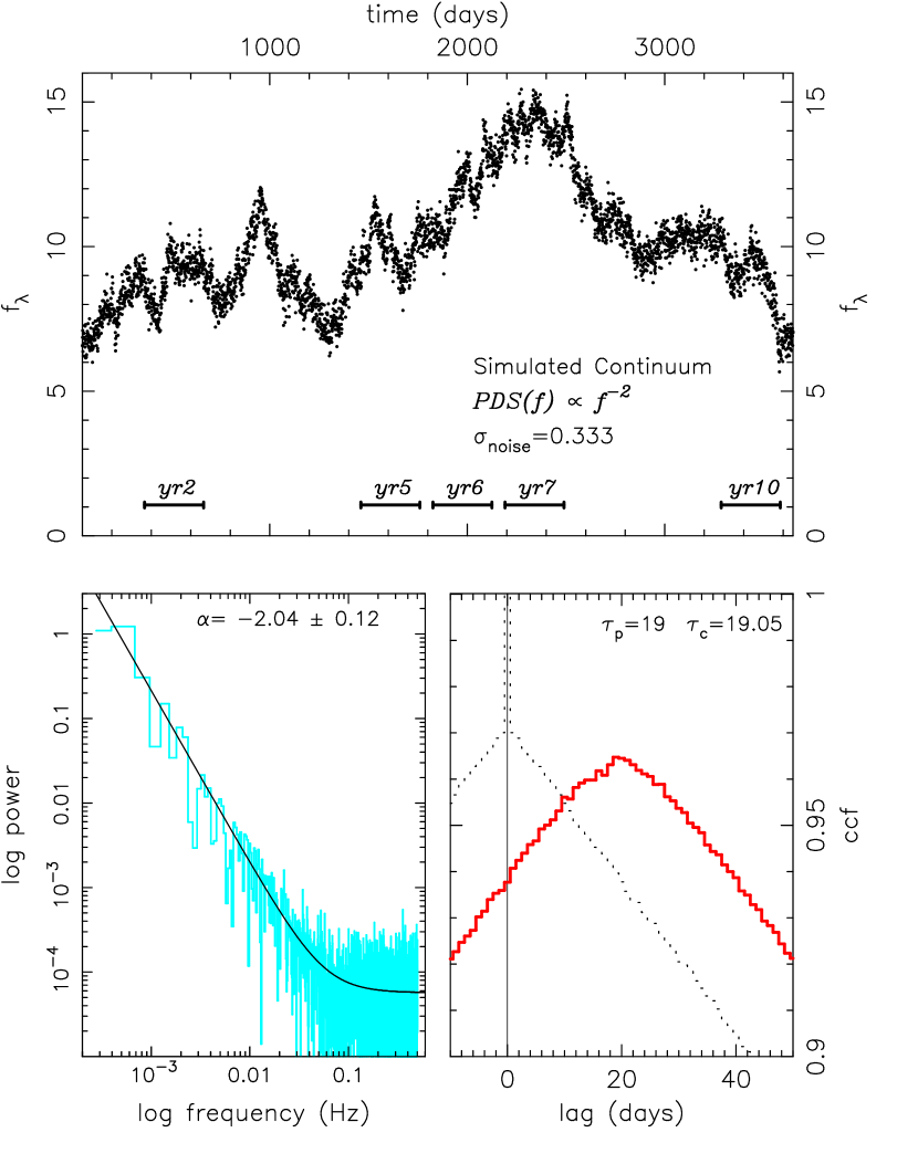
The line light curve is generated by convolving the original noise–free and zero–mean with . The line light curve is then scaled to give an rms value of 1.5 (in units of erg s-1 cm-2) and a constant of 7.5 is added. Gaussian distributed white noise with a standard deviation of 0.30 is then added to the line light curves to mimic observational noise. The parameters are summarized in Table 1, along with the actual observed values for NGC 5548 from Peterson et al. (1999). Figure 1 shows a typical 10–year long simulated continuum light curve, along with its local ACF and PDS.555Technical note: all PDS were computed using linearly detrended and Welch tapered light curves. The two lowest frequency bins were not used in the fit to the PDS. The local CCF between the simulated continuum and line light curve for the entire 10 yr period is also shown.
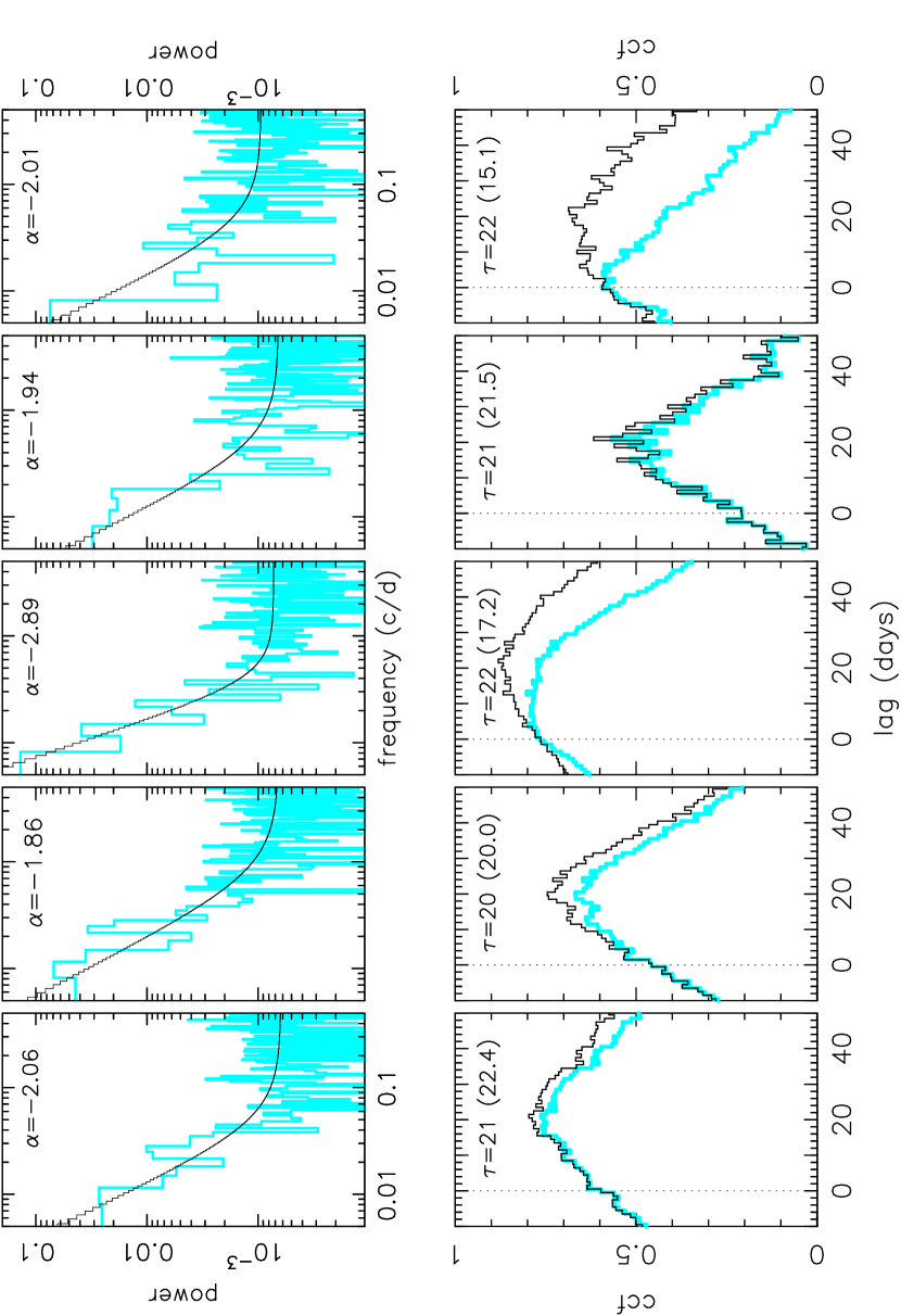
The light curve is then broken into 10 isolated segments, each 300 days long. Each of these segments corresponds to a season’s worth of simulated AGN data. Note that each continuum light curve is independent — the mean, the rms variability, the ACF, and the PDS are not fixed. Figure 2 shows the PDS and CCFs for five seasons extracted from the light curve in Fig. 1. Notice the large changes in shape and lag of the CCFs in these examples, all of which were taken from the same parent light curve. Also notice the differences between the standard and local CCFs.
To build up a statistical number of realizations, the above construction process was repeated 100 times, yielding 1000 seasons of independent simulated continuum and line light curves. The standard and local methods were used to compute the CCF for each of the 1000 pairs of light curves. Both the peak of the CCF and the centroid position were recorded; as in Peterson, et al. 1999, only values of the CCF that lie above 0.8 times the maximum r value were used in the centroid determination.
4.2 Simulation Results
4.2.1 The local vs. standard CCF
Figures 3 and 4 show the peak lag values for each of the 1000 trials, along with their CCPD, i.e., a histogram of the lag values. Results from the local CCF method (Fig 3), and the standard CCF definition (Fig 4) are shown. The superiority of the local method is immediately evident. These figures also illustrate two points: (1) there is a downward bias in the CCF, so that the average or median value underestimates the true lag of 20 d; (2) the scatter of the CCF peaks is very large.
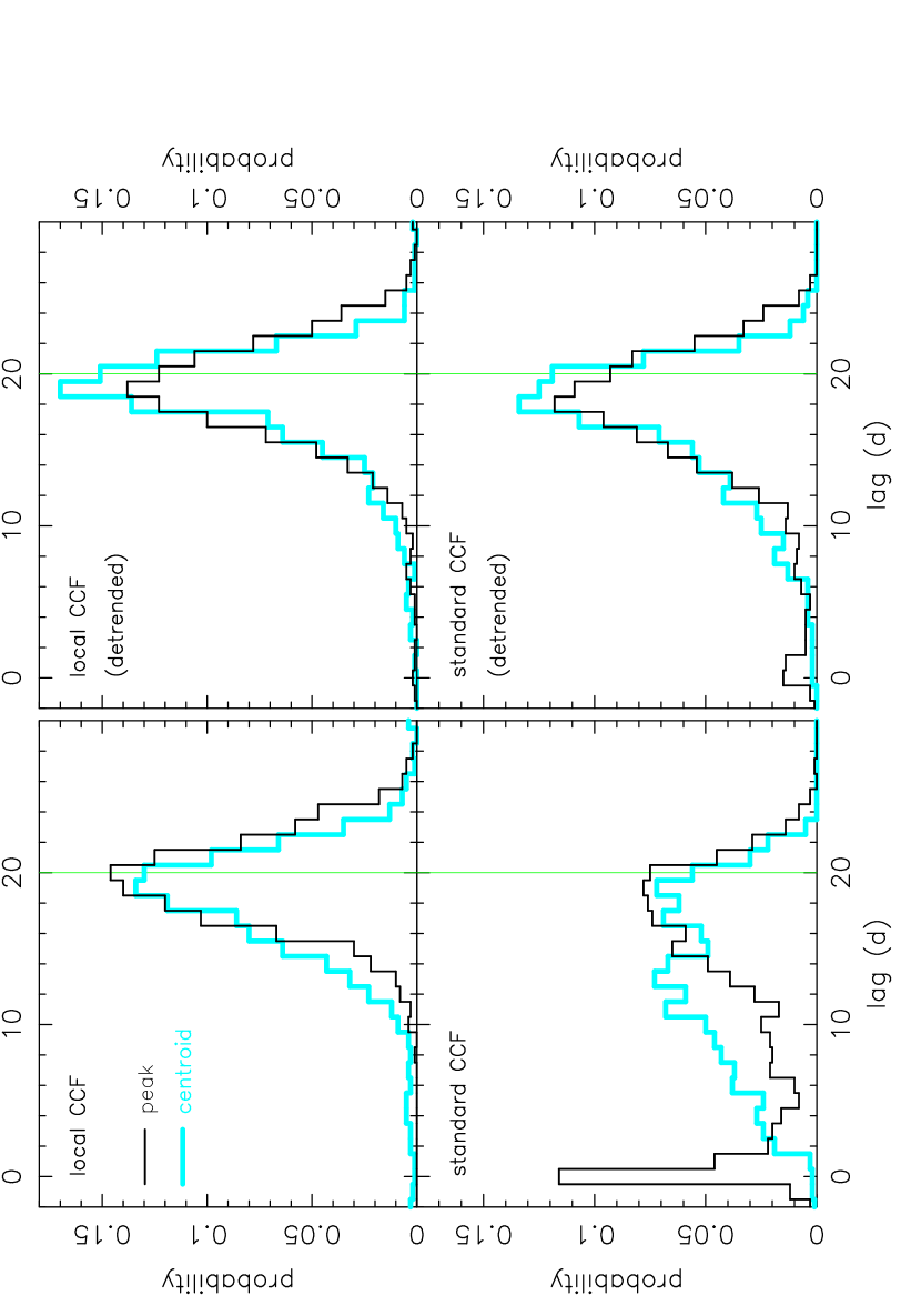
In Fig. 5, eight different CCPD are shown, each resulting from a different method of computing the lag, but all from the same 1000 pairs of light curves. On the left, the peak and centroid lags are shown for the local and standard CCF methods. The right panels show the same but for light curves that have had a linear fit subtracted prior to computing the CCF. This figure reveals several features: all CCPD show a downward bias, and this bias is very severe for the standard CCF method; the centroid distributions are more susceptible to bias than the peak distributions; the linear detrending greatly improves the standard method, but only slightly improves the local method (because the local method inherently contains a high–pass filter). The large number of CCFs that peak at zero delay in the standard CCF are due to trends in those season’s light curves: a strong linear trend in both continuum and line light curves will dominate the CCF. Linear detrending of each season’s light curves is therefore highly beneficial.
The simulations described above are optimistic in several regards: (i) the light curves are equally sampled with no gaps, (ii) the observational noise–induced scatter in fluxes are purely independent and Gaussian, (iii) the transfer function has a well–defined peak, and (iv) the duration of the light curves are 15 times longer than the lag of the peak of the transfer function. As a result, the conclusions drawn from these simulations are robust — more realistic simulations would show a larger scatter.
It was noticed that on occasion, the line ACF was narrower than the continuum ACF. This has sometimes been seen in AGN light curves and suggests that contains negative values or is non–linear (see the discussion by Sparke 1992). However, it can simply be a side–effect of finite duration sampling.
4.2.2 The effects of the continuum power spectrum “color”
To test the sensitivity to the assumed PDS power–law exponent , we carried out simulations using parent continuum light curves with a and PDS. The peaks of the local CCFs were determined, after the light curves had linear trends removed. The results are shown in Figs. 6 and 7, where it is clear that the scatter in the lags depends strongly on the value of . This is because the width of the ACF is sensitive to : redder PDS (more negative ) have broader ACFs. As stated in eq. (5), the ideal CCF is identical to the transfer function convolved with the ACF, so a broad ACF yields a broad CCF whose peak is poorly defined. The consequence is that the redder the continuum fluctuations, the more the ability to infer properties of from the measured CCF degrades. These simulation can be compared with the three model CCFs shown in Fig. 4 of Edelson & Krolik (1988), where redder continuum light curves yield a stronger correlation, but contain less structure and hence less information.
The above claim that the CCF peak should be more easily measured for whiter PDS leads to an apparent contradiction. The transfer function acts similarly to a low–pass filter, hence high frequency variations present in the continuum are averaged out and are not seen in line light curve. The thicker the BLR, the more the high frequencies are lost. This suggests that a continuum light curve dominated by low frequencies, i.e., a very red PDS, would provide a better “driver” for echo mapping. Indeed, this effect is seen by White & Peterson (1994) in their CCPD comparisons using and simulated continuum light curves. The contradiction is resolved by noting that the signal–to–noise ratio of typical AGN variability data is rather low, hence noise in the light curves is important. For continuum light curves with equal intrinsic rms variability but different PDS power–law slopes, the deleterious effect of white noise is more pronounced for whiter PDS. In other words, the S/N is timescale dependent: low frequency variations have effectively a higher S/N than high frequency variations. Since convolution with the transfer function preserves low–frequency power, continuum light curves with redder PDS yield CCFs that are are less sensitive to noise. However, one cannot escape the fact that a very red PDS continuum will have a very broad ACF and CCF, making its peak and centroid determinations difficult. For high S/N data, a whiter PDS will enable a richer echo mapping analysis.
4.2.3 The duration of the light curves
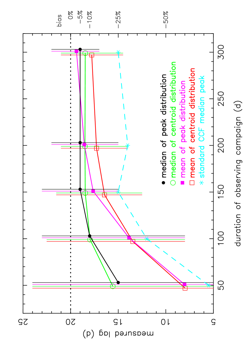
As the duration of the time series increases, one expects the reliability of CCF lag determination to improve. To quantify this behavior, Figure 8 shows the mean and median lag values plotted as a function of the length of the hypothetical observing campaign. Five curves are drawn, corresponding to the mean and median for the peaks and centroids of the local CCFs, and the median of the peaks using the standard CCF method. As before, 1000 simulations were used to determine the mean and median, and these simulations were identical in all respects except for the number of points. While all the distributions encompass the true value within , they are all biased too low. For simulations that match the characteristics of the observations of NGC 5548, the lag is underestimated by 5% using the local CCF method.
From this figure it is clear that the median is a far better statistic than the mean. This is because large outliers are not rare. For light curves of 150–300 days duration, the median bias in the local CCFs is roughly 5–10%. For shorter duration light curves, the bias and variance increase rapidly: for 100 day long time light curves the bias is 10% and for 50 day long light curves the bias grows to 25%. For light curves this short the huge uncertainty in the lag makes a single estimate almost meaningless. For comparison, the standard CCF method produces significantly more biased values: even with 300–day long light curves the bias is 25%.
The commonly held belief that the time series used to compute the CCF should be at least 4 times longer than the lags of interest, and preferably 10 times longer, is illustrated in this figure. As the light curves lengthen, the lags only asymptotically approach the unbiased value. Extending a 200 day long light curve by 100 days does not decrease the bias nearly as much as extending a 100 day long light curve by the same amount. Once the light curves exceed about 10 times the lag, increasing the S/N of the data leads to more significant improvements then extending the duration of the light curves.
4.2.4 The signal–to–noise ratio
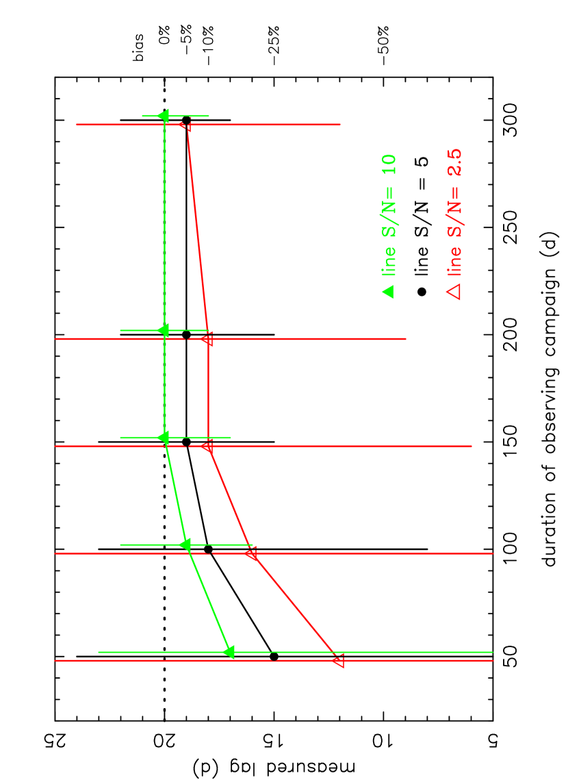
The previous simulations were all based on a line S/N of 5, mimicking the NGC 5548 H observations. S/N is defined here as the ratio of intrinsic line rms variations to the simulated observational noise per datum — see Table 1 for the numerical values. To quantify the effects of a change in S/N, Fig. 9 shows the median of the CCPD for S/N values of 2.5, 5 and 10, plotted as functions of the duration of the light curves. For this figure, lag is defined as the peak of the local CCF. Both the line S/N and the continuum S/N were boosted by the same factors, achieved in realization by reducing the amount of added simulated observational noise.
As expected, the higher the S/N, the smaller the bias, and more importantly, the smaller the variance about the median. From this figure it can be deduced that under certain conditions, doubling the S/N of the individual observations can be as significant as doubling the duration of the light curves.
4.2.5 The effects of detrending
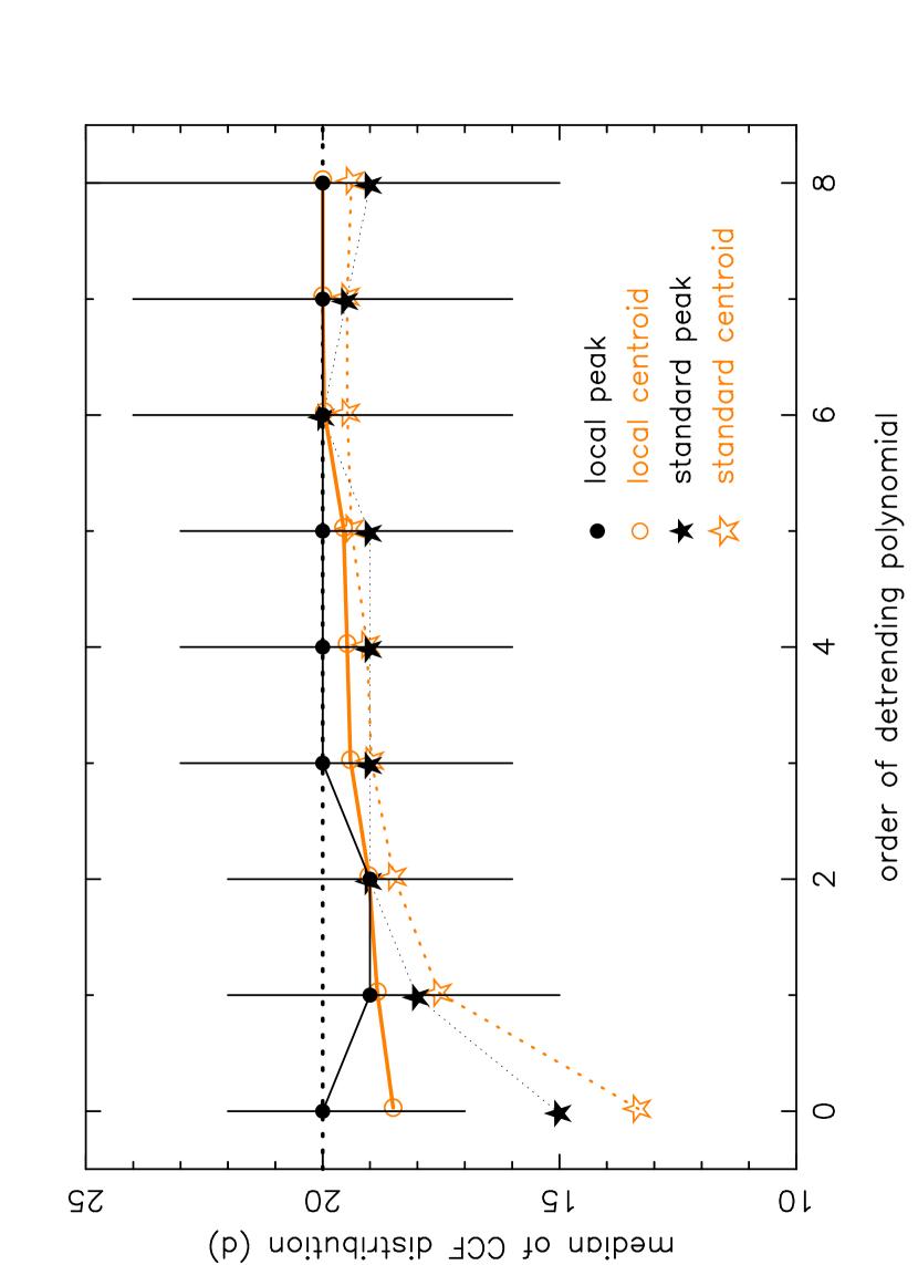
In §3.1.4, 3.1.7, and 4.2.1 it was stated that “detrending” or removing low frequency power from the light curves can improve CCF lag determinations. Figure 10 explicitly shows this effect. Plotted are the median values of the 1000 CCF simulations versus the order of the polynomial used to remove trends from the light curves (order 0 = mean, order 1 = linear, order 2 = quadratic, etc.). The detrending was accomplished by least–squares fitting a polynomial to the entire light curve for the observing season (300 days in all cases) then subtracting off the polynomial prior to computing the CCF. In all cases identical light curves were used (with a line S/N = 5). For clarity, only the error bars for the median lag computed with the local CCF are shown. In general, as the order of the polynomial increases, the bias in the CCF decreases.
For the standard method, simply removing a linear trend can result in a substantially better estimate of the lag. Significant additional improvements can be made by going to a 3rd or 4th order polynomial. However, for higher orders, the variance increases, offsetting the benefits of detrending.
The beneficial effect of detrending is more pronounced for the standard CCF method than for the local method because the local method intrinsically contains a detrending–like filter (see §3.1.5). Nevertheless, the local method also benefits from low–order polynomial detrending of the light curves. (The apparent degrading of the local CCF median when going from no detrending to linear detrending is a statistical event. More typically, the median value with no detrending is equal to or worse than with linear detrending.) Figure 10 again illustrates that the local CCF outperforms the standard CCF, and that the peak is a better (less biased) estimator than the centroid. However, the local CCF is more noisy than the standard CCF, particularly at large lags, and this grows worse with higher order detrending.666In the situation where outliers become common at the largest lags the median is no longer a good statistic to use to characterize the CCPD, since it depends on the limits of where the lags are computed (i.e., the median becomes sensitive to the endpoints of the interval over which the CCF is computed). A better statistic would be the mode or the center of a narrow Gaussian fit to the distribution.
Conceptually, detrending works for the following reason: AGN light curves have a red power spectrum, so most of the signal in the light curves are contained in the lowest frequencies. However, these low frequencies are the most poorly sampled in the light curve: there is only one measurement of the lowest Fourier frequency, two of the second lowest frequency, and so on. Due to the small number of samples, statistical fluctuations are very important. This is in contrast to the high frequency power, where there are many samples, but the observational noise is large (or even dominant). Detrending the light curves with polynomials applies a smooth and gently rolling high–pass filter.777For equally sampled data a sharp, well–defined high-pass filter could be applied in the Fourier domain, but for unequally sampled data working in the Fourier domain is problematic. The CCF will no longer be dominated by poorly sampled low frequencies, and hence less prone to random fluctuations. The scatter in the CCF is therefore reduced. Another way to think of it is that the detrending sharpens the ACFs, and since the CCF is approximately the ACF convolved with the , the CCF sharpens up.
To understand why detrending reduces bias, one must realize that the CCF is extremely efficient at finding the lag if the time series PDS are white; otherwise the CCF can give poor results. For example, if the time series contains a trend then for a long time interval the data will tend to be above (or below) the mean. Thus the data values are not randomly distributed about the mean; instead they are highly correlated on long timescales. This correlation will dominate the CCF and the peak of the CCF will occur at (or near) zero lag. Thus there is a bias towards small lags if there is any low frequency power in the time series. For example, the peak of the standard CCF will occur at zero lag for any two linear light curves. Unless the deviations from the straight lines are large, the CCF will tend to peak at zero lag.
AGN light curves are dominated by low frequency power hence the CCF will be biased towards too small lags unless the data are “pre–whitened”.888Determining radial velocity shifts of lines in a flux spectrum does not suffer as much bias because the power spectrum of the flux spectrum is mostly white. Nevertheless, any trends in the continuum must be removed or the resulting radial velocities will be biased. Detrending the light curves via polynomials is one way of removing low frequency power; other methods include subtracting off splines or a moving average, applying a differencing operation (see e.g. Chatfield 1996), or directly multiplying by a high–pass filter in the Fourier domain. Since AGN light curves are red, it is clear that some form of pre–whitening should be carried out.
What order polynomial should be used to detrend the light curves? The answer depends on the characteristics of the data: the redder (more negative ) the power spectra, the more detrending is required; the lower the S/N, the less detrending can be tolerated. AGN light curves have power at all observed frequencies so there will always be linear and other low–frequency trends, independent of the duration of the light curve. The minimum order of the detrending polynomial is therefore insensitive to the length of the light curve: a linear trend should always be removed. A crude estimate for the maximum order can be made as follows. A polynomial of order has at most zeroes, so it removes power on timescales greater than where is the duration of the time series. For a reliable CCF estimate, a light curve with a duration of 5–10 times the lag timescale is necessary. This gives a polynomial of order 0.4–0.5 , where is the lag expected for the given transfer function. If the S/N is poor, the maximum order polynomial for detrending will be less than this. When the light curves are heavily detrended, much of the intrinsic signal in the data is removed, leaving lower and lower S/N data for the CCF to work with. The lag of the peaks of the CCFs will therefore not necessarily converge with increasing detrending. In the extreme limit where the filtering leaves only the observational white noise, the ACF again will peak at zero lag because of correlated noise between the continuum and line observations (since they are both measured from the same spectrum). So while the detrending removes bias, it also increases the variance, and in extreme limits it re–introduces a bias. For this reason, large amounts of detrending is not beneficial. The technique of differencing the data (see §3.1.4) removes all low–frequency trends, and hence is not a viable option for data that is not of exceptionally high S/N.
The strong recommendation that results from this work is that removal of low–frequency trends in the light curves can significantly improve the reliability of the CCF lag determinations. Removal of a linear trend is essential; removal of a cubic or quartic trend is recommended; higher orders may be useful if the correlation remains strong enough to provide an unambiguous determination of the peak. In practice, one should compute and compare the CCF for progressively larger amounts of detrending.
4.2.6 The effects of tapering
Tapering (also called “windowing”) a time series is common practice in Fourier analysis (see, e.g., Jenkins & Watts 1968; Press et al. 1996). Tapering helps compensate for “end effects” of a finite duration time series: a sampled time series can be thought of as the product of two time series, the “true” infinite duration time series and a time series whose value is unity during the data acquisition interval and zero elsewhere. The multiplication of the true time series with this sampling function is identical to convolution of the Fourier transform of the true time series with the Fourier transform of a boxcar. The result is that the Fourier transform is broadened by convolution with a sinc function. The broadening results in “leakage” of power from one frequency into other frequency bins. Tapering the light curves consists of multiplying the light curves with a function that slowly goes from zero to unity and back over the duration of the experiment. The new time series has “softer” edges that produce a Fourier transform with less leakage. For time series that have a red power spectra, the leakage of power from low frequencies to higher frequencies is significant, and possibly even dominant at if the intrinsic PDS is redder than . Because of the equivalence of the CCF with its discrete Fourier transform counterpart, reducing leakage from low to high frequencies should improve the CCF lag estimate. The red PDS of AGN light curves means leakage is significant and suggests that tapering the light curves can have a benefical effect.
To explore the possible benefits of tapering, simulations were carried out using light curves that were detrended and tapered prior to computing the CCF. The taper was applied in two ways: (1) a global taper, applied once to the entire light curve; (2) a local taper, applied to each overlapping segment pair. The global taper is more akin to what is used to reduce spectral leakage; the local taper forces the same taper to be applied independent of lag.
The results indicate that tapering does on average improve the reliability of the CCF lag estimate. However, the effect is small compared to the effect produced by detrending. As expected, the greater the amount of detrending, the less effect the tapering had. The two different methods of tapering (global and local) produced similar results for small lags; the differences were much less than the variance in the estimates of the lag. For globally tapered light curves, the local and standard methods of computing the CCF gave very similar results for small lags. For large lags, the global taper significantly reduces the amplitude of the CCF. This has two effects: (1) it greatly reduces the number of outliers in the CCPD; (2) it introduced a strong bias against finding a correlation at a large lag. Provided the light curves are long compared to the true lag (something that is not known a priori), the latter effect is not serious. In summary, tapering does have a beneficial effect and the benefits are not very sensitive to the specific method of tapering (or taper shape), but the effect of detrending is far more important. In practice, one should compute the CCF several ways: using the standard and local method, different amounts of detrending, and with and without tapering.
5 Discussion and Conclusion
We have discussed some properties of the cross correlation function, specifically in the AGN echo mapping context. The two main issues we address are (1) the bias in the CCF and (2) the uncertainties in the CCF lag determinations. Both of these stem from finite duration sampling of the light curves, not irregular/sparse sampling or observational noise. Bias can also be introduced if low frequency power dominates the light curves. Since AGN light curves have a red power spectrum, this second source of bias is also present.
Because of the bias problem the CCF fails on average to reproduce the correct lag. The bias is inherent in the definition of the standard CCF itself and depends strongly on the ratio of the intrinsic (true) lag to the duration of the observed light curves and also the sharpness of the continuum autocorrelation function and transfer function. Unfortunately the amount of bias cannot be determined from the data themselves, i.e., one needs to know the true CCF in order to calculate the bias. As a result, exact corrections are impossible and simulations are required to estimate the statistical size of the bias. However, much of the bias can be removed by simply detrending (and to a lesser extent tapering) the light curves.
The impact on AGN variability studies is that the standard CCF tends to underestimate the true time lag, therefore the derived characteristic radius for the BLR is underestimated. From simulations designed to mimic the well–sampled light curves of NGC 5548, the estimated lag is too low by 5–10%; for more poorly sampled light curves the bias can be much larger. This bias amplitude is based on using the “local” CCF method, in which the means and standard deviations used to calculate the CCF are determined using only those parts of the light curves that overlap at for a given lag. We find that the local CCF gives superior results compared to the standard definition of the CCF, where the bias can be 3 times larger. Although the size of the bias is relatively small compared to the intrinsic uncertainty in the measured lags of many AGN, as the quality of the data continues to improve, the bias will not be negligible and its effect should not be ignored.
We also find that the lag of the centroid of the CCF does not yield a more accurate representation of the BLR size because (1) it is more heavily biased than the peak of the CCF; (2) unlike the infinite case, the centroid of the sample CCF does not necessarily correspond to the centroid of the transfer function.
It has been observed that the H lag in NGC 5548 changes from year to year (Peterson et al. 1999) and this can be interpreted in several ways. The variations can be attributed to the AGN itself, e.g., the BLR structure may be evolving, or the illumination of the BLR by the photoionizing source may be changing (Wanders & Peterson 1996), or the engine producing the continuum variability is changing such that the continuum ACF is variable. However, an alternate explanation is simply that the changing CCF lag is due to finite duration sampling of the light curves. Simulations that mimic the optical continuum and H observations of NGC 5548 demonstrate that, even with perfect sampling and with a transfer function that has a well–defined peak, the scatter in measured CCF lags is large. Thus the scatter in the observed lags in NGC 5548 can be attributed to finite duration sampling of a random process.
Observations have shown that AGN flux time series are not stationary on timescales spanning several observing seasons, i.e., the means and variances of the light curves do not remain constant from year to year. Since the continuum variability properties are not constant (in particular the ACFs), one cannot use the observed CCFs to unambiguously deduce changes in the transfer function.
It is of course possible that the changing lag is intrinsic to the AGN, but we have shown that the scatter in the lags are also consistent with the interpretation of being a consequence of finite duration sampling of a random walk–like process. Our simulations produce a distribution of lags that is as wide as the observed scatter. Given that the artificial data were oversampled, equally sampled, had perfectly known noise characteristics and a transfer function with a well–defined peak, the results of the simulations are highly robust.
To determine if the observed lag variations are intrinsic to the AGN, one needs to show that a realistic simulation produces a narrower scatter in lag distribution than what is observed, or that yearly changes in the lags are not random. Given that much longer observing runs than what has already been obtained for NGC 5548 are not feasible, the resolution of the question of the significance of the changing lags will demand new data with much higher S/N. This would substantially tighten the scatter in the simulated lag distributions, while its effect on the observed scatter depends on if the variations are intrinsic or not. Also, a better understanding of the continuum variability characteristics such as the power spectrum power–law exponent would allow more realistic simulations. As we have shown, the scatter in the simulated lag distribution depends strongly on the power law slope of the power spectrum. In this regard, a Fourier analysis of the long–term NGC 5548 continuum light curve is warranted.
Finally, enumerated below are some practical suggestions that can improve the reliability of CCF lag determinations in AGN: (1) Detrending the light curves produces far more reliable CCFs. Linear detrending is required, and higher order detrending can be beneficial if the S/N is high; (2) The peak of the CCF gives a more reliable lag estimate than the centroid. (3) Tapering the light curves also has a beneficial effect, though not as significant as detrending; (4) The “local CCF” is less biased and therefore gives better results than the standard CCF, especially for small lags. However, if the light curves are detrended and tapered, the advantage the local CCF has over the standard CCF is small. If simulations are used to estimate uncertainties in the lag estimates, then: (5) The median of the CCPD is more reliable than the mean or mode for light curves that are not too heavily detrended; (6) An improvement of the bootstrap + Monte Carlo method (Peterson et al. 1999a) as described in §3.2 should be used. However, simulations of this nature can only yield an estimate of the uncertainty of the lag for that particular sample of light curve. Without an understanding of the true ACF itself (not the sample ACF), estimates based on resampling or perturbing the observed sample light curves can underestimate the variability of the lag.
References
- Alexander (1997) Alexander, T. 1997, in Astronomical Time Series, ed. D. Maoz, A. Sternberg, and E.M. Leibowitz (Dordrecht: Kluwer), p. 163
- Bevington & Robinson (1992) Bevington, P.R. & Robinson D.K. 1992, “Data Reduction and Error Analysis for the Physical Sciences”, 2nd ed. (:WCB/McGraw–Hill)
- Blandford & McKee (1984) Blandford, R.D., & McKee, C.F. 1982 ApJ 255, 419
- Box, Jenkins & Reinsel (1994) Box, G.E.P., Jenkins, G.M. & Reinsel, G.C. 1994, “Time series Analysis: Forecasting and Control”, 3rd ed. (Englewood Cliffs:Prentice–Hall)
- Chatfield (1996) Chatfield, C. 1996, “The Analysis of Time Series: An Introduction”, Fifth edition (London:Chapman & Hall)
- Clavel, et al. (1987) Clavel, J., et al. 1987, ApJ, 321, 251
- Clavel, et al. (1991) Clavel, J., et al. 1991, ApJ, 366, 64
- Diaconis & Efron (1983) Diaconis, P. & Efron, B. 1983, Sci. Amer., 248, 116
- Edelson & Krolik (1988) Edelson, R.A. & Krolik, J.H. 1988, ApJ, 333, 646
- Efron (1983) Efron, B. 1983, “The Jackknife, the Bootstrap, and Other Resampling Plans”, CBMS-NSF Regional Conference Series in Applied Mathematics 38, Society for Industrial and Applied Mathematics
- Gaskell & Peterson (1987) Gaskell, C.M. & Peterson, B.M. 1987, ApJS, 65, 1
- Gaskell & Sparke (1986) Gaskell, C.M. & Sparke, L.S. 1986, ApJ, 305, 175
- Gondhalekar, Horne & Peterson (1994) Gondhalekar, P.M., Horne, K. & Peterson, B.M. (eds.) 1994, “Reverberation Mapping of the Broad–Line Region in Active Galactic Nuclei” (San Francisco: ASP)
- Horne (1994) Horne, K. 1994, in “Reverberation Mapping of the Broad–Line Region in Active Galactic Nuclei”, P.M. Gondhalekar, K. Horne & B.M. Peterson (eds.) (San Francisco: ASP) p. 23
- Horne, Welsh & Peterson (1991) Horne, K., Welsh, W.F. & Peterson, B.M. 1991, ApJ, 367, L5
- Jenkins & Watts (1969) Jenkins, G.M. & Watts, D.G. 1969, “Spectral Analysis and its Applications”, (San Francisco:Holden–Day)
- Kendall (1954) Kendall, M.G. 1954, Biometrika, 41, 403
- Koen (1994) Koen, C. 1994, MNRAS, 268, 690
- Koen (1993) Koen, C. 1993, MNRAS, 262, 823
- Koratkar & Gaskell (1991a) Koratkar, A.P. & Gaskell, C.M. 1991a, ApJS, 75, 719
- Koratkar & Gaskell (1991b) Koratkar, A.P. & Gaskell, C.M. 1991b, ApJ, 375, 85
- Krolik & Done (1995) Krolik, J. H. & Done, C. 1995, ApJ, 440, 166
- Krolik, et al. (1991) Krolik, J.H., Horne, K., Kallman, T.R., Malkan, M.A., Edelson, R.A. & Kriss, G.A. 1991, ApJ, 371, 541
- Litchfield, Robson & Hughes (1995) Litchfield, S.J., Robson, E.I. & Hughes, D.H. 1995, AA, 300, 385
- Maoz & Netzer (1989) Maoz, D. & Netzer, H. 1989, MNRAS, 236, 21
- Marriot & Pope (1954) Marriott, F.H.C. & Pope, J.A. 1954, Biometrika, 41, 390
- Netzer & Peterson (1997) Netzer, H. & Peterson, B.M. 1997, in Astronomical Time Series, ed. D. Maoz, A. Sternberg, and E.M. Leibowitz (Dordrecht: Kluwer), p. 85
- Otnes & Enochson (1978) Otnes, R.K. & Enochson, L. 1978, “Applied Time Series Analysis — Vol. 1 Basic Techniques”, (NY: John Wiley & Sons, Inc.)
- Penston (1991) Penston, M.V. 1991, in Variability in active galactic nuclei, eds. H. Richard Miller and Paul J. Wiita (Cambridge: CUP), p. 343
- Pérez (1992) Pérez, E., Robinson, A., & de la Funete, L. 1992, MNRAS, 255, 502
- Peterson (1988) Peterson, B.M. 1988, PASP, 100, 18
- Peterson (1993) Peterson, B.M. 1993, PASP, 105 247
- Peterson, et al. (1998a) Peterson, B.M., Wanders, I., Horne, K., Collier, S., Alexander, T., Kaspi, S. & Maoz, D. 1998a, PASP, 110, 660
- Peterson, et al. (1998b) Peterson, B.M., Wanders, I., Bertram,R., Huntley, J.F., Pogge, R.W. & Wagner, R.M. 1998b, ApJ, 501, 82
- Peterson, et al. (1985) Peterson, B.M., et al. 1985, ApJ, 292,164
- Peterson, et al. (1994) Peterson, B.M., et al. 1994, ApJ, 425, 622
- Peterson, et al. (1999) Peterson, B.M., et al. 1999, ApJ, 510, 659
- (38) Pijpers, F.P. & Wanders, I. 1994, MNRAS, 271, 183
- Press, et al. (1996) Press, W.H., Flannery, B.P., Teukolsky, S.A., & Vetterling, W.T. 1996, “Numerical Recipes in Fortran 77: The Art of Scientific Computing (Vol. 1 of Fortran Numerical Recipes)”, (Cambridge: Cambridge Univ. Press)
- Press, Rybicki & Hewitt (1992) Press, W.H., Rybicki, G.B. & Hewitt, J.N. 1992, ApJ, 385, 404
- Reichert, et al. (1994) Reichert, G.A., et al. 1994, ApJ, 425, 582
- Robinson & Perez (1990) Robinson, A. & Pérez, E. 1990, MNRAS, 244, 138
- Rodriguez–Pascual, et al. (1989) Rodríguez–Pascual, P.M., Santos–Leó, M. & Clavel, J. 1989, AA, 219, 101
- Scargel (1989) Scargle, J.D. 1989, ApJ, 343, 874
- Sparke (1993) Sparke, L.S. 1993, ApJ, 404, 570
- Sutherland, Weisskopf & Kahn (1978) Sutherland, P.G., Weisskopf, M.C. & Kahn, S.M. 1978, ApJ, 219, 1029
- Tjostheim & Paulsen (1983) Tjostheim, D. & Paulsen, J. 1983, Biometrika, 70, 389
- Ulrich, Maraschi & Urry (1997) Ulrich, M.–H., Maraschi, L. & Urry, C.M. 1997, ARAA, 35,445
- Vio, Horne & Wamsteker (1994) Vio, R., Horne, K. & Wamsteker W. 1994, PASP, 106, 1091
- Wade & Horne (1988) Wade, R.A. & Horne, K. 1988, ApJ, 324, 411
- Wall (1996) Wall, J.V. 1996, QJRAS, 37, 519
- Wanders & Peterson (1996) Wanders, I. & Peterson, B.M. 1996, ApJ, 466, 174
- White & Peterson (1994) White, R.J. & Peterson, B.M. 1994, PASP, 106, 879


| Simulations | NGC 5548aaderived from Peterson, et al. (1999) | ||||||
|---|---|---|---|---|---|---|---|
| Continuumbbcontinuum fluxes are in units of erg s-1 cm2 Å-1. | HccH line fluxes are in units of erg s-1 cm2. | Continuum | H | ||||
| mean flux | 10.0 | 7.5 | 9.35 1.86 | 7.56 1.53 | |||
| intrinsic rms flux | 2.0 | 1.5 | 1.82 | 1.50 | |||
| 20% | 20% | 19.5% | 19.9% | ||||
| observational noise | 0.333 | 0.30 | 0.33 | 0.28 |