Chemo-spectrophotometric evolution of spiral galaxies:
III. Abundance and colour gradients in discs

Abstract

We study the relations between luminosity and chemical abundance profiles of spiral galaxies, using detailed models for the chemical and spectro-photometric evolution of galactic discs. The models are “calibrated” on the Milky Way disc and are successfully extended to other discs with the help of simple “scaling” relations, obtained in the framework of semi-analytic models of galaxy formation. We find that our models exhibit oxygen abundance gradients that increase in absolute value with decreasing disc luminosity (when expressed in dex/kpc) and are independent of disc luminosity (when expressed in dex/scalelength), both in agreement with observations. We notice an important strong correlation between abundance gradient and disc scalelength. These results support the idea of “homologuous evolution” of galactic discs.

1 Introduction

Almost all large spiral galaxies present sizeable radial abundance gradients. This is, for instance, the case for the Milky Way disc, showing an oxygen abundance gradient of dlog(O/H)/dR$\sim$-0.07 dex/kpc in both its gaseous and stellar components. The origin of these gradients is still a matter of debate. A radial variation of the star formation rate (SFR), or the existence of radial gas flows, or a combination of these processes, can lead to abundance gradients in discs (e.g. Lacey and Fall 1985, Koeppen 1994, Edmunds and Greenhow 1995, Tsujimoto et al. 1995, Firmani et al. 1996, Molla et al. 1997, Matteucci and Chiappini 1998). On the other hand, the presence of a central bar inducing large scale mixing through radial gas flows tends to level out preexisting abundance gradients (e.g. Dutil and Roy 1999). Despite several studies in the 90ies (e.g. Friedli et al. 1998 and references therein) the relative importance of these processes has not been clarified yet.

Several large spectophotometric surveys and literature compilations have appeared in recent years (Vila-Costas and Edmunds 1992, Zaritsky et al. 1994, Garnett et al. 1997, van Zee et al. 1998). These studies allowed to establish several important features of abundances in spirals (Henry and Worthey 1999, and references therein). In particular, it is established now that the absolute abundance at a given galactocentric distance is correlated to galaxy luminosity (and rotational velocity). Also, when abundance gradients are expressed in dex/kpc there is a tendency of smaller discs to exhibit larger gradients; but when they are expressed in dex/R_d (where R_d is the disc exponential scalelength), that correlation disappears (Garnett et al. 1997).

In a series of recent papers (Boissier and Prantzos 1999a, 1999b; hereafter BP99a and BP99b, respectively) we presented a detailed model of the chemical and spectrophotometric evolution of spiral galaxies. Adopting some simple prescriptions for the star formation and infall rates, we first applied the model to the Milky Way disc and showed that it reproduces all major observables of our Galaxy (BP99a), including radial profiles of gas, stars, SFR and oxygen abundances. Assuming that the Milky Way is a typical spiral galaxy, we extended then the model to the study of other spirals (BP99b) with the help of some simple “scaling laws”, which have been established in the framework of the Cold Dark Matter scenarios for galaxy formation. We showed that this simple “scaled” model reproduces quite satisfactorily most of the observed integrated properties of present day spirals: disc sizes and central surface brigthness, Tully-Fisher relations in various wavelength bands, colour-colour and colour-magnitude relations, gas fractions vs. magnitudes and colours, abundances vs. local and integrated properties, as well as spectra for different galactic rotational velocities. Despite the extremely simple nature of our models, we find satisfactory agreement with all those observables, provided the timescale for star formation in low mass discs is longer than for more massive ones.

In this third paper of the series we explore the implications of our models for the radial profiles of spiral galaxies and, in particular, the abundance and photometry gradients. The plan of the paper is as follows: In Sec. 2 we present the basic ingredients and the underlying assumptions of the model. The results of the models concerning the evolution of the radial oxygen abundance profiles and the final abundance and luminosity gradients are presented in Sec. 3. In Sec. 4 we compare our results to observations; in particular, we show that there is a clear correlation between abundance gradient expressed in dex/kpc and disc scalelength, both observationnaly and in our models. The implications of these results for disc evolution are discussed in Sec. 5.

2 The model

In this section we recall the main ingredients and the underlying asumptions of our chemical and spectrophotometric evolution models.

The galactic disc is simulated as an ensemble of concentric, independently evolving rings, gradually built up by infall of primordial composition. The chemical evolution of each zone is followed by solving the appropriate set of integro-differential equations (Tinsley 1980), without the Instantaneous Recycling Approximation. Stellar yields are from Woosley and Weaver (1995) for massive stars and Renzini and Voli (1981) for intermediate mass stars. Fe producing SNIa are included, their rate being calculated with the prescription of Matteucci and Greggio (1986). The adopted stellar Initial Mass Function (IMF) is a multi-slope power-law between 0.1 M_⊙ and 100 M_⊙ from the work of Kroupa et al. (1993).

The spectrophotometric evolution is followed in a self-consistent way, i.e. with the SFR $\Psi(t)$ and metallicity $Z(t)$ of each zone determined by the chemical evolution, and the same IMF. The stellar lifetimes, evolutionary tracks and spectra are metallicity dependent; the first two are from the Geneva library (Schaller et al. 1992, Charbonnel et al. 1996) and the latter from Lejeune et al. (1997). Dust absorption is included according to the prescriptions of Guiderdoni et al. (1998) and assuming a “sandwich” configuration for the stars and dust layers (Calzetti et al. 1994).

The star formation rate (SFR) is locally given by a Schmidt-type law, i.e proportional to some power of the gas surface density $\Sigma_{g}$ and varies with galactocentric radius $R$ as:

$$\Psi(t,R)\ =\ \alpha\ \Sigma_{g}(t,R)^{1.5}\ V(R)\ R^{-1}$$ (1)

where $V(R)$ is the circular velocity at radius $R$. This radial dependence of the SFR is suggested by the theory of star formation induced by density waves in spiral galaxies (e.g. Wyse and Silk 1989).

The infall rate is assumed to be exponentially decreasing in time, i.e.

$$f(t,R)\ =\ A(R)\ e^{-t/\tau(R)}$$ (2)

with $\tau(R_{0}$=8 kpc) = 7 Gyr in the solar neighborhood, in order to reproduce the local G-dwarf metallicity distribution. The coefficient $A(R)$ is obtained by the requirement that at time T=13.5 Gyr the current mass profile of the disc $\Sigma(R)$ is obtained, i.e.

$$\int_{0}^{T}f(t,R)\ =\ \Sigma(R)$$ (3)

with

$$\Sigma(R)\ =\ \Sigma_{0}\ e^{-R/R_{d}}$$ (4)

In the case of the Milky Way disc one has for the central surface density $\Sigma_{0}$=1150 M_⊙ pc^-2 and for the disc scalelength $R_{d}$=2.6 kpc, leading to an overall disc mass $M_{d}\sim$5 10¹⁰ M_⊙ (see BP99a and references therein).

The efficiency $\alpha$ of the SFR (Eq. 1) is fixed by the requirement that the observed local gas fraction $\sigma_{g}(R_{0}$=8 kpc)$\sim$0.2, is reproduced at T=13.5 Gyr. We consider then that the really “free” parameters of the model are the radial dependence of the infall timescale $\tau(R)$ and of the SFR. It turns out that the number of observables explained by the model is much larger than the number of free parameters. In particular the model reproduces present day “global” properties (profiles of gas, O/H, SFR, and supernova rates), as well as the current disc luminosities in various wavelength bands and the corresponding radial profiles of gas, stars, SFR and metal abundances; moreover, the adopted inside-out star forming scheme leads to a scalelength of $\sim$4 kpc in the B-band and $\sim$2.6 kpc in the K-band, in agreement with observations (see BP99a).

Figure 1: Evolution of oxygen abundance profiles in our models, at times t=3 Gyr (dotted curves), 7.5 Gyr (dash-dotted curves) and 13.5 Gyr (solid curves). Models are arranged according to values of maximum rotational velocity $V_{C}$ (increasing from top to bottom) and spin parameter $\lambda$ (increasing from left to right). In the case of the Milky Way model ($V_{C}$=220 km/s, $\lambda$=0.03) observations of oxygen abundances in HII regions, planetary nebulae and B-stars are also plotted; the observed metallicity gradient dlog(O/H)/dR$\sim$-0.07 dex/kpc is well reproduced. Notice that the absolute values of $\lambda$ do not enter directly the calculations, since the model discs are scaled to the one of the Milky Way through the relations (5) and (6); in other terms, if the Milky Way $\lambda$ is taken to be 0.06, the same results would be obtained for discs with $\lambda$ = 0.02, 0.06, 0.10, 0.14 and 0.18, respectively.

In order to extend the model to other disc galaxies we adopt the “scaling properties” derived by Mo, Mao and White (1998, hereafter MMW98) in the framework of the Cold Dark Matter (CDM) scenario for galaxy formation. According to this scenario, primordial density fluctuations give rise to haloes of non-baryonic dark matter of mass $M$, within which baryonic gas condenses later and forms discs of maximum circular velocity $V_{C}$. It turns out that disc profiles can be expressed in terms of only two parameters: rotational velocity $V_{C}$ (measuring the mass of the halo and, by assuming a constant halo/disc mass ratio, also the mass of the disc) and spin parameter $\lambda$ (measuring the specific angular momentum of the halo). In fact, a third parameter, the redshift of galaxy formation (depending on galaxy’s mass) is playing a key role in all hierarchical models of galaxy formation. However, since the term “time of galaxy formation” is not well defined (is it the time that the first generation of stars form? or the time that some fraction of the stars, e.g. 50% form?) we prefer to ignore it and assume that all discs start forming their stars at the same time, but not at the same rate. In that case the profile of a given disc can be expressed in terms of the one of our Galaxy (the parameters of which are designated hereafter by index G):

$$\frac{R_{d}}{R_{dG}}\ =\ \frac{\lambda}{\lambda_{G}}\ \frac{V_{C}}{V_{CG}}$$ (5)

and

$$\frac{\Sigma_{0}}{\Sigma_{0G}}\ =\left(\frac{\lambda}{\lambda_{G}}\right)^{-2}\ \frac{V_{C}}{V_{CG}}$$ (6)

where we have adopted $\lambda_{G}$=0.03 (see BP99b). Numerical simulations show that the $\lambda$ distribution peaks around the value 0.04 (e.g. MMW98). The absolute value of $\lambda_{G}$ is of little importance as far as it is close to that peak, since our results depend only on the ratio $\lambda/\lambda_{G}$.

Eqs. 5 and 6 allow to describe the mass profile of a galactic disc in terms of the one of our Galaxy and of two parameters: $V_{C}$ and $\lambda$. The range of observed values for the former parameter is 80-360 km/s, whereas for the latter numerical simulations give values in the 0.01-0.1 range, the distribution peaking around $\lambda\sim 0.04$ (MMW98). Although it is not clear yet whether $V_{C}$ and $\lambda$ are independent quantities, we treat them here as such and construct a grid of 25 models caracterised by $V_{C}$ = 80, 150, 220, 290, 360 km/s and $\lambda$ = 0.01, 0.03, 0.05, 0.07, 0.09, respectively. [Notice: if $\lambda_{G}$=0.06 is adopted for the Milky Way, our model results would be the same, but they would correspond to values of $\lambda$ twice as large, i.e. 0.02, 0.06, 0.10, 0.14 and 0.18, respectively]. Increasing values of $V_{C}$ correspond to more massive discs and increasing values of $\lambda$ to more extended discs.

As discussed in BP99b, the resulting disc radii and central surface brightness are in excellent agreement with observations, except for the case of $\lambda$=0.01. This “unphysical” value leads to galaxies ressembling to bulges or ellipticals, rather than discs. We prefer, however, to keep this $\lambda$ value in our grid, for illustration purposes.

The two main ingredients of the model, namely the Star Formation Rate $\Psi(R)$ and the infall time-scale $\tau(R)$, are affected by the adopted scaling of disc properties in the following way:

For the SFR we adopt the prescription of Eq. (1), with the same efficiency $\alpha$ as in the case of the Milky Way (i.e. the SFR is not a free parameter of the model). In order to have an accurate evaluation of $V(R)$ across the disc, we calculate it as the sum of the contributions of the disc (with the surface density profile of Eq. 4) and of the dark halo, with a volume density profile of a non-singular isothermal sphere (see BP99b).

The infall time scale is assumed to increase with both surface density (i.e. the denser inner zones are formed more rapidly) and with galaxy’s mass, i.e. $\tau[M_{d},\Sigma(R)]$. In both cases it is the larger gravitational potential that induces a more rapid infall. The radial dependence of $\tau$ on $\Sigma(R)$ is calibrated on the Milky Way, while the mass dependence of $\tau$ is adjusted as to reproduce several of the properties of the galactic discs (see BP99b). The adopted prescription allows to keep some simple scaling relations for the infall in our models and the number of free parameters as small as possible. The fact that the adopted simple prescription provides a satisfactory agreement with several observed relationships in spirals (see BP99b) makes us feel that it could be ultimately justified by theory or numerical simulations of disc formation.

We stress at this point that in our models we ignore the possibility of radial inflows in gaseous discs, resulting e.g. by viscosity or by infalling gas with specific angular momentum different from the one of the underlying disc; in both cases, the resulting redistribution of angular momentum leads to radial mass flows. The magnitude of the effect is difficult to evaluate, because of our poor understanding of viscosity and our ignorance of the kinematics of the infalling gas. Models with radial inflows have been explored in the past (Mayor and Vigroux 1981; Lacey and Fall 1986; Clarke 1989; Chamcham and Tayler 1994); at the present stage of our knowledge, introduction of radial inflows in the models would imply even more free parameters and make impossible the study of a radial variation in the efficiency of the SFR. Since it is well known that bars induce radial mixing and reduce the abundance gradients (e.g. Dutil and Roy 1999), we do not consider bared galaxies in what follows.

3 Results and comparison to observations

3.1 Model results

The evolution of the oxygen abundance profiles in our models is presented in Fig. 1. Profiles are shown at three ages: T=3, 7.5 and 13.5 Gyr, respectively, covering most of the galaxian history. It should be noticed that the observed oxygen profile in the Milky Way disc is nicely reproduced by the corresponding model ($V_{C}$=220 km/s, $\lambda$=0.03), as analysed in detail in BP99a. The most important features of Fig. 1 are the following:

1) Because of the inside-out star forming scheme adopted in our work, the abundance profile is quite steep early on (when stars and metals are formed only in the inner disc) and flattens with time (as star formation “migrates” progressively outwards).

2) The final abundance gradients (expressed in dex/kpc) are, in general, larger for the lower mass discs. The reason is that, in such small galaxies, the $\Sigma_{g}^{1.5}/R$ factor in the adopted SFR can create large differences in abundances between regions relatively close to each other. Indeed, because of the small scalelength of these galaxies, the gas surface density varies a lot within a short distance, and so does the corresponding SFR. On the contrary, for massive and large discs, the gas surface density and corresponding SFR vary slowly within one kpc and produce flatter abundance gradients (in dex/kpc).

Figure 2: Results of our models at an age T=13.5 Gyr. They are plotted as a function of maximal rotational velocity $V_{C}$ and spin parameter $\lambda$ (0.03 solid curves, 0.05 dotted curves, 0.07 short-dashed curves and 0.09 long-dashed curves). From top to bottom: oxygen abundance gradient (in dex/kpc); absolute B-magnitude M_B; disc scalelength in the B-band R_B; radius where B-band surface brightness is 25 mag arcsec^-2 (R₂₅); colour gradient B-K (in mag/kpc). In all panels, the symbol $\odot$ indicates values corresponding to the Milky Way model.

3) The more massive the galaxy, the higher is the central (and average) abundance. This is due to the $V/R$ factor of the adopted SFR, making massive discs more efficient in forming stars and metals at a given galactocentric distance. This factor explains also why the most compact discs ($\lambda$=0.01) have very high abundances. However, as analysed in BP99b, that case does not produce “physical” results, since the obtained galaxies ressemble more to ellipticals or bulges than to spirals. We show the results for $\lambda$=0.01 in Fig. 1 for illustration purposes, but in the following we shall discuss only results for the other cases. In BP99b we show that this increase of metallicity with disc mass and luminosity compares well to the data of Zaritsky et al. (1994).

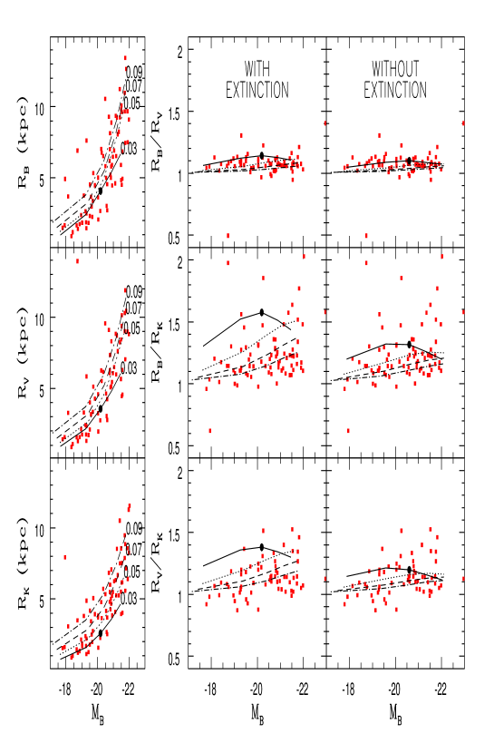
Figure 3: Disc scalelengths in various wavelength bands (left) and disc scalelength ratios (middle and right) as a function of B-magnitude. Our results (curves, parametrised with values of the spin parameter $\lambda$ as indicated on the left) are compared to the observations of de Jong (1996). Model scalelengths in the middle panels are calculated with extinction taken into account, while in the right panels extinction is neglected. In all panels, the filled circle indicates results for the Milky Way disc.

4) The most efficient galaxies in forming stars and metals are the compact (low $\lambda$) and massive (large $V_{C}$) ones. In their innermost regions, metallicity tends to saturate, to a value of log(O/H)+12$\sim$9.4. This is a well known feature of galactic chemical evolution models taking into account the finite lifetime of stars (see Prantzos and Aubert 1995). At late times, when most of the gas is exhausted and little star formation or metal production takes place, large amounts of metal-poor gas are returned to the interstellar medium; they are ejected by the numerous low-mass and long-lived stars that were abundantly formed in the early days of the galaxy. This metal-poor gas dilutes the metal abundances and leads to a “saturation” of their value. This feature cannot be revealed by models using the Instantaneous Recycling Approximation. For that reason, the oxygen profiles of the $\lambda$=0.01 case are flat, since star formation is very rapid and efficient all over the (small) disc.

Figure 2 summarizes a number of important features of our models at an age of T=13.5 Gyr.

a) The oxygen abundance gradient (in dex/kpc) is a monotonically increasing function of $V_{C}$. Notice that gradients are negative and more massive discs have smaller absolute values of d(log(O/H))/dR, i.e. flatter abundance profiles. Also, abundance gradients depend on the $\lambda$ value, especially in low mass discs: more compact discs have more important (in absolute value) gradients, while extended discs have flat abundance profiles. In both cases, the fact that smaller discs have larger abundance gradients (in dex/kpc) is due to the $\Sigma^{1.5}$/R factor in the adopted star formation rate, as explained in point 2 above.

b) The B-magnitude depends mainly on the mass of the galaxy (i.e. rotational velocity $V_{C}$) and very little on the spin parameter $\lambda$. As analysed in detail in BP99b, a Tully-Fisher relation with a slope similar to the observed one in field spirals and small dispersion is obtained in our models. This is a success of semi-analytical models, since the TF relation is “built-in” as a boundary condition (the disc mass being proportional to $V_{C}^{3}$).

c) The final B-band scalelength is a monotonically increasing function of $V_{C}$ and $\lambda$. This again is due to the “boundary conditions” imposed by the semi-analytic models adopted in our work (see Sec. 2).

d) R₂₅, the radius where B-band surface brightness is 25 mag/arcsec², is also found to increase monotonically with $V_{C}$ and $\lambda$.

e) Finally, discs with $\lambda>0.05$ have small colour gradients, independently of their mass (lower panel in Fig. 2). This is because in those galaxies the whole disc is formed relatively late (in timescales $>$5 Gyr for $V_{C}<$220 km/s, see Fig. 5 in BP99b) and stellar populations in the inner disc are not much older than in the outer regions.

3.2 Comparison to observations of luminosity profiles

The exponential scalelength of the Milky Way disc was a subject of controversy for several years. Indeed, observations in different wavelength bands lead to different results: a value of R${}_{B}\sim$4-5 kpc is found in the B-band, while smaller values are found in longer wavelengths (R${}_{I}\sim$2.5 kpc). In BP99a we showed that these different values result naturally from schemes of “inside-out” formation of the disc, that manage to reproduce the observed oxygen abundance gradient of dlog(O/H)/dR$\sim$-0.07 dex/kpc. In fact, light in the I- or K- bands traces closely the old stellar population, which dominates the mass of the disc in all radii. Light in the B-band traces a younger stellar population, formed in the past 1-2 Gyr from a gas with a surface density profile flatter than the one of the old population. Thus, colour and abundance gradients are found to be naturally correlated in the case of the Milky Way disc.

In this section we explore the results of our models concerning the disc scalelengths in various wavelength bands. Our aim is: 1) to see whether our results are compatible with the observations and 2) to check whether there are any similarities with the case of the Milky Way.

On the left part of Fig. 3 we present the disc scalelength of our models in the B-, V- and K- bands (evaluated with the effects of extinction taken into account) and compare them to the observations of De Jong (1996). De Jong has decomposed the luminosity profiles of his $\sim$80 face-on galaxies in bulge and disc components and we plot in Fig. 3 only the corresponding disc component, directly comparable to our results. It can be seen that the model disc scalelengths are in excellent agreement with the observed ones as a function of M_B. More massive and bright discs have larger scalelengths on the average, while the variation of the spin parameter $\lambda$ allows to reproduce the observed scatter (perhaps not quite efficiently in the B-band).

On the right part of Fig. 3 we plot the disc scalelength ratios as a function of M_B. Since extinction may affect the results, we plot our results with extinction included (middle panels) and neglected (right panels). It can be seen that the observed R_B/R_K and R_V/R_K rates are on the average larger than 1 (i.e. there is a colour gradient); also, there is a marginal trend of increasing ratios with galaxy luminosity. Our results are in agreement with the observed trends, in particular when extinction is included. We find that the case of $\lambda$=0.03 leads to the most extreme scalelength ratios; other $\lambda$ values (i.e. less compact discs) produce more modest colour gradients. In that respect then, our Milky Way is a rather compact disc having larger than average colour gradients.

3.3 Comparison to observations of abundance gradients

In this section we compare our results to the observations of Garnett et al. (1997) and van Zee et al. (1998) concerning abundance gradients in external spirals (i.e. observations of O/H in HII regions as a function of galactocentric distance).

Figure 4: Oxygen abundance gradients of our models at T=13.5 Gyr (open symbols, corresponding to the values of the spin parameter $\lambda$ as indicated in the upper panel and connected with solid curves). They are plotted as a function of the B-magnitude and compared to observations (filled symbols, with appropriate references given in each panel). Upper panel: Oxygen gradient in dex/kpc; Middle panel: Oxygen gradient in dex/R_B; Lower panel: Oxygen gradient in dex/R₂₅.

Garnett et al. (1997) combine data obtained in several previous works (Vila-Costa and Edmunds 1992, Zaritsky et al. 1994 and Ryder 1995) and make several adjustements in order to introduce a greater degree of uniformity. From this final sample we selected a sub-sample of 17 non-barred galaxies, since those compare better to our models (bars can induce mixing of gas along the disc and flattening of abundance gradients in relatively short timescales, e.g. Friedli et al. 1998 and references therein; our models do not take such effects into account). On the other hand, van Zee et al. (1998) combine data from the literature (including their own observations for low metallicity HII regions) and derive abundance gradients for 11 more spirals.

Our results are compared to observations in Fig. 4, where abundance gradients are plotted as a function of integrated B-magnitude.

In the upper panel, abundance gradients are expressed in dex/kpc. Observations show that luminous discs have small gradients, while as we go to low luminosity ones the absolute value of the gradients and their dispersion increase. This trend is fairly well reproduced by our models. The reason can be understood by comparing to the upper panel of Fig. 2, where our results are plotted as a function of $V_{C}$ (which correlates well to M_B through the Tully-Fisher relation, BP99b). As analysed in Sec. 3.1, the $\Sigma_{g}^{1.5}$/R factor in the adopted SFR creates large abundance variations within short distances in small galaxies; no important gradients can be created in massive discs, where neighboring regions differ little in $\Sigma_{g}$. As for the increased dispersion at low luminosities (and low $V_{C}$), it is due to the effect of the $\lambda$ parameter: for large $\lambda$ values, even small mass discs are quite extended (Eq. 5 in Sec. 2) and the $\Sigma^{1.5}$/R factor becomes less and less efficient in creating abundance gradients (since $\Sigma$ varies little as a function of R). Thus, in low mass discs, both the mass and the spin parameter $\lambda$ drive the abundance gradient.

As stressed in BP99b, discs with $\lambda>0.08$ correspond to Low Surface Brightness galaxies (LSBs, see also Jimenez et al. 1998). According to DeBlok and van der Hulst (1998) LSBs have negligible abundance gradients. Our results of Fig. 4 are quite encouraging in that respect: indeed, had we run models with $\lambda>0.09$ we would expect to find smaller and smaller abundance gradients at all galaxy luminosities. We postpone, however, the detailed study of LSBs in a forthcoming paper.

In the middle panel of Fig. 4, the oxygen gradients are expressed in dex/R_B. When expressed in this unit, the observed abundance gradients show no more any correlation to M_B, as already noticed in Garnett et al. (1997). Moreover, a considerable dispersion is obtained for all M_B values, while the average gradient is $\sim$-0.2 dex/R_B. Our results (values in the upper panel of Fig. 2, multiplied by the corresponding R_B values of the middle panel of Fig. 2) show also no correlation with M_B, in fair agreement with observations. However, the average value is slightly larger than observed ($\sim$-0.25 dex/R_B). Since the estimates of R_B, both in observations and in our models, may be affected by extinction, we consider that the agreement with the data is quite satisfactory. Another difficulty may stem from the fact that relatively few discs can be fit with perfect exponentials; according to Courteau and Rix (1999) this happens for only $\sim$20% of the disc galaxies. Finally, we obtain no significant dispersion in our models, contrary to obervations. We suspect that the difficulties to evaluate the effects of extinction or to fit the profiles with a perfect exponential may be (at least partly) responsible for the observed scatter.

In the lower panel of Fig. 4 abundance gradients are expressed in dex/R₂₅. Again, observations show no trend with M_B and a considerable dispersion. Our results also show no correlation with M_B, while the average model value ($\sim$-0.8 dex/R₂₅) is in perfect agreement with observations. This is most encouraging, since $R_{25}$ is less affected by considerations on dust extinction or fit to an exponential profile. Indeed, we think that the obtained average value of dlog(O/H)/dR=-0.8 dex/R₂₅ is a more robust result than the -0.25 dex/R_B value obtained in the previous paragraph. However, the observed dispersion is not reproduced by our models; only part of it can be attributed to the effects of the spin parameter $\lambda$.

Figure 5: Predictions of our models for the gradients of metallicity (in dex/kpc) vs 1/R_B (left panels) and 1/R₂₅ (right panels). In the upper panels our models are parametrised by $V_{C}$ values and in the lower panels by $\lambda$ values. Data are from Garnett et al. (1997), van Zee et al. (1998) and Zaritsky et al. (1994). A clear correlation is found between abundance gradient (in dex/kpc) and 1/R_B.

3.4 Abundance and colour gradients vs. scalelength

In the previous section it was shown that:

a) abundance gradients (in dex/kpc) become more important and present a larger dispersion in low luminosity discs.

b) Abundance gradients in dex/R_B are independent of disc luminosity, and so is the corresponding dispersion.

Points (a) and (b) immediately suggest that there must be a one-to-one correlation between abundance gradients and scalelength R_B. The correlation must be relatively tight, since the observed dispersion (middle panel of Fig. 4) is relatively small. Although this conclusion is an immediate consequence of the observations in Fig. 4, it has never been stated explicitly (to our knowledge). For the same reason, a one-to-one correlation must exist between abundance gradients and R₂₅. However, the observed scatter (lower panel in Fig. 4) shows that one should not expect a very tight correlation in that case.

In Fig. 5 we plot the oxygen abundance gradients (in dex/kpc) as a function of 1/R_B (which is proportional to a “magnitude gradient” in mag/kpc) and of 1/R₂₅, both from observations and from our models. In the upper panels our results are parametrised by the values of rotational velocity $V_{C}$, while in the lower panels they are parametrised by the values of the spin parameter $\lambda$. It can be seen that our models show an excellent correlation between the abundance gradients and 1/R_B: smaller discs have larger gradients and the results depend little on $\lambda$. In principle, knowing the B-band scalelength of a disc, one should be able to determine the corresponding abundance gradient and vice-versa! In practice, however, observations show a scatter around the observed trend. Moreover, our results seem to agree better with the data of Garnett et al. (1997) than with those of van Zee et al. (1998). The latter show a less steep dependence of the gradient on 1/R_B. Since large discs “cluster” on the upper left corner of the diagram, we suggest that observations of the abundance gradients in small discs would help to establish the exact form of the correlation. Finally, we notice that in our models we find similar correlations between abundance gradients and disc scalelengths in other wavelength bands (as can be expected from the fact that scalelength ratios are close to unity, Fig. 3).

The situation is not as promising when abundance gradients are plotted as a function of 1/R₂₅. Our models show again a correlation, but this time the different $\lambda$ values lead to increasingly different abundance gradients as one goes to smaller discs. Although the data are compatible with the obtained relation, the large observational uncertainties do not allow to conclude. Again, further observations for small discs are required to clarify the situation.

Figure 6: Predictions of our models at T=13.5 Gyr for the relation between metallicity gradient (in dex/kpc) and colour gradient B-K (in mag/kpc). The grid of our models is parametrised by $V_{C}$ (360, 290, 220, 150 and 80 km/s, from top to bottom) and $\lambda$ (0.03, 0.05, 0.07 and 0.09, from left to right). Massive and extended discs have negligible metallicity and colour gradients.

Finally, our models predict that, in general, colour gradients are developped in discs, because of the inside-out star formation scheme. For instance, in the case of the Milky Way we obtain R${}_{B}\sim$4 kpc and R${}_{K}\sim$2.6 kpc, in agreement with observations (see BP99a and references therein). As shown in Fig. 2 (bottom panel) and discussed in Sec. 3.1, colour gradients are rather small for discs with $\lambda>$0.05; only for low $\lambda$ and $V_{C}$ values do they become important. In Fig. 6 we present the obtained relationship between abundance and B-K gradient, expressed in dex/kpc and mag/kpc, respectively. Although the resulting grid covers a rather large part of the figure, it nevertheless excludes the co-existence of large colour and small abundance gradients. Combined chemical and photometric analysis of disc profiles should allow to find out whether the proposed scheme is realistic or not.

4 Summary

In this work, we study the photometric and chemical abundance profiles resulting from our models of the evolution of galactic discs. Our galaxy evolution models are calibrated on the Milky Way (BP99a) and reproduce a large body of observational data concerning integrated properties of external spirals (BP99b). Here it is shown that they also produce results in excellent agreement with observations of abundance gradients in spiral galaxies. More specifically:

1) Because of the inside-out star formation scheme, our models predict that abundance and photometric profiles flatten with time.

2) Model abundance gradients (in dex/kpc) are more important and present a larger dispersion for low luminosity discs, in fair agreement with observations. We claim that the spin parameter $\lambda$ (affecting the size, but not the mass of the disc in our models) is responsible for the scatter. Discs with larger $\lambda$ values than those studied here should appear as Low Surface Brightness galaxies and should exhibit even smaller abundance gradients than those displayed in Fig. 3. Observations show indeed that LSBs have negligible abundance gradients (DeBlok and van der Hulst, 1998).

3) When expressed in dex/R_B and dex/R₂₅, observed abundance gradients show no dependence on galaxy luminosity; they do show an important scatter, especially in the latter case. Our models also show no trend with luminosity, while the average values are in fair agreement with observations. We fail, however, to reproduce the observed scatter (variations induced by the different $\lambda$ values are not sufficient for that).

4) The observed and theoretical relation between galaxy luminosity and abundance gradients, suggest that there must also exist a correlation between the latter and 1/R_B or 1/R₂₅. Our models show indeed such a correlation: abundance gradients (in dex/kpc) correlate much better to 1/R_B than to M_B. Observations seem to coroborate this idea, although more data are needed to establish the precise form of that correlation.

5) Our models show no correlation between abundance and colour gradients (expressed in dex/kpc and mag/kpc, respectively), except for the most compact discs (those with $\lambda$=0.03). Compact discs of low luminosity are found to have large abundance and colour gradients.

The most interesting feature of this work is the anticorrelation found between abundance gradients and scalelength. Discs with small scalelengths have large abundance gradients, independently of their mass. It is the first time (to our knowledge) that this relationship is noticed. It should be interesting to establish it through further observations, concerning in particular discs of small scalelengths. Our models seem to reproduce that relationship quite naturally (Fig. 5).

We wish to stress here that our simple chemical evolution models treat galactic discs as ensembles of concentric, independently evolving rings, i.e. no radial flows ar considered. If radial inflows are indeed playing a key role in shaping abundance gradients (as sometimes claimed), how is then the success of our models to be understood?

As explained in Sec. 2, our models are “calibrated” on the Milky way disc. In particular, the radial dependence of the adopted infall rate is such that, when combined to the adopted SFR, reproduces the current profiles of gas, stars and metal abundances. The fact that we keep the same prescriptions for the SFR and infall rate in the other disc models, leads obviously to a kind of “homologuous evolution”, as already suggested in Garnett et al. (1997). In other words, prescriptions adopted for the Milky Way are found to be equally successful when applied to other discs. It should be interesting to see whether hydrodynamical simulations (like e.g. those of Samland et al. 1997, or Contardo et al. 1998) manage to produce this kind of “homologuous evolution” in galactic discs. We notice, however, that the idea of a “homologuous evolution” merely states a fact, but does not itself explain the origin of the observed gradients.

References

- [Boissier & Prantzos1999] Boissier S. & Prantzos N., 1999a, MNRAS, 307, 857 (BP99a)
- [Boissier & Prantzos1999] Boissier S. & Prantzos N., 1999b, MNRAS in press and astro-ph/9909120 (BP99b)
- [] Calzetti D., Kinney A. & Storchi-Bergmann T., 1994, ApJ,429,582
- [1] Chamcham C. & Tayler R., 1994, MNRAS, 266, 282
- [Charbonnel et al.1996] Charbonnel C., Meynet G., Maeder A. & Schaerer D., 1996, A&AS, 115,339
- [2] Clarke C., 1989, MNRAS, 238, 283
- [] Contardo G. , Steinmetz M. & Fritze-Von Alvensleben U., 1998, ApJ, 507, 497
- [Courteau & Rix1999] Courteau S. & Rix H.-W., 1999, ApJ, 513, 561
- [] DeBlok W. & van der Hulst J., 1998, A&A, 335, 421
- [] De Jong R., 1996, A&A Suppl., 118, 557
- [] Dutil Y. & Roy J.-R., 1999, ApJ, 516, 62
- [] Edmunds M. & Greenhow R., 1995, MNRAS, 272, 241
- [] Firmani C., Hernandez X. & Gallagher J., 1996, A&A, 308, 403
- [] Friedli D., Edmunds M., Robert C. & Drissen L., 1998, “Abundance Profiles: Diagnostic Tools for Galaxy History”, ASP Conf. Series 147
- [] Garnett D., Shields G., Skillman E., Sagan S. & Dufour R.,1997, ApJ, 489, 63
- [Guiderdoni et al.1998] Guiderdoni B., Hivon E., Bouchet R. & Maffei B., 1998, MNRAS, 295,877
- [] Henry R. & Worthey G., 1999, PASP, 111, 919
- [] Jimenez R., Padoan P., Matteucci F. & Heavens A., 1998, MNRAS, 299, 123
- [] Koeppen J., 1994, A&A, 281, 26
- [Kroupa et al.1993] Kroupa P., Tout C. & Gilmore G., 1993, MNRAS, 262, 545
- [] Lacey C. & Fall S., 1985, ApJ, 290, 154
- [] Lejeune T., Cuisinier F. & Buser R., 1997, A&AS, 125,229
- [] Matteucci F. & Chiappini C., 1998, ESO Conference “Chemical Evolution from Zero to High Redshift”, held in Garching. Aph/9812315.
- [Matteucci & Greggio] Matteucci F. & Greggio L., 1986, A&A, 154, 279
- [3] Mayor M. & Vigroux L., 1981, A&A, 98, 1
- [Mo et al.1998] Mo H., Mao S. & White S., 1998, MNRAS, 295,319
- [Molla et al.1997] Molla M., Ferrini F. & Diaz A., 1997, ApJ, 475, 519
- [] Prantzos N. & Aubert O., 1995, A&A, 302, 69
- [Renzini & Voli1981] Renzini A. & Voli A., 1981, A&A, 94, 175
- [] Ryder S., 1995,ApJ, 444, 610
- [] Samland M., Hensler G. & Theis C., 1997, ApJ, 476, 544
- [] Schaller G., Schaerer D., Maeder A. & Meynet G., 1992, A&AS, 96, 269
- [] Tinsley B., 1980, Fund. Cosm. Phys., 5, 287
- [] Tsujimoto T., Yoshii Y.,Nomoto K. & Shigeyama T., 1995, 302, 704
- [] Van Zee L., Salzer J., Haynes M., O’Donoghue A. & Balonek T., 1998, AJ, 116, 2805
- [] Vila-Costas M. & Edmunds M., 1992, MNRAS, 259, 121
- [Woosley & Weaver1995] Woosley S. & Weaver T., 1995, ApJ Suppl., 101. 181
- [Wyse & Silk1989] Wyse R. & Silk J., 1989, ApJ, 339, 700
- [] Zaritsky D., Kennicutt R. & Huchra J.,1994, ApJ, 420,87