The infrared polarizations of high-redshift radio galaxies

Abstract

This thesis reports the $K$-band polarizations of a representative sample of nine radio galaxies: seven 3C objects at $0.7<z<1.3$, and two other distinctive sources. Careful consideration is given to the accurate measurement and ‘debiasing’ of faint polarizations, with recommendations for the function of polarimetric software.

  3C 22

has 3% polarization perpendicular to its radio structure, consistent with suggestions that it may be an obscured quasar.

  3C 41

also has 3% polarization perpendicular to its radio and may also be an obscured quasar; its scattering medium is probably dust rather than electrons.

  3C 54

is polarized at 6%, parallel to its radio structure.

  3C 65

is faint: its noisy measurements give no firm evidence for polarization.

  3C 114

has a complex structure of four bright knots, one offset from the radio structure and three along the axis. There is strong evidence for polarization in the source as a whole (12%) and the brightest knot (5%).

  3C 356

is faint: we do not detect any $K$-band continuation of the known visible/near-ultraviolet polarization.

  3C 441

lies in a rich field; one of its companions appears to be 18% polarized. The identification of the knot containing the active nucleus has been disputed, and is discussed.

  LBDS 53W091

was controversially reported to have a 40% $H$-band polarization. No firm evidence is found for non-zero $K$-band polarization in 53W091, though there is some evidence for its companion being polarized. The object is discussed in the context of other radio-weak galaxies.

  MRC 0156$-$252

at $z\sim 2$ is found to be unpolarized in $K$.

Simple spectral and spatial models for polarization in radio galaxies are discussed and used to interpret the measurements. The important cosmological question of the fraction of $K$-band light arising in radio galaxy nuclei is considered: in particular, the contribution of scattered nuclear light to the total $K$-band emission is estimated to be of order 7% in 3C 22 and 3C 41, 26% in 3C 114, and tentatively 25% or more in 3C 356.

Declarations required by the University of Wales

Declaration
This work has not previously been accepted in substance for any degree, and is not being concurrently submitted in candidature for any degree.

$\>\overline{~{}~{}~{}~{}\mbox{\rule{0.0pt}{11.56346pt} Candidate \hskip 332.44243pt Date }}\>$

Statement 1
This thesis is the result of my own investigations, except where otherwise stated as indicated by footnotes to the text. All sources consulted are referenced and a full bibliography is appended.

$\>\overline{~{}~{}~{}~{}\mbox{\rule{0.0pt}{11.56346pt} Candidate \hskip 332.44243pt Date }}\>$

Statement 2
I hereby give consent for my thesis, if accepted, to be available for photocopying and inter-library loan, and for the title and summary to be made available to outside organisations. On acceptance, a copy of the thesis will be lodged in the astro-ph archive at xxx.soton.ac.uk and its mirror sites on the internet.

$\>\overline{~{}~{}~{}~{}\mbox{\rule{0.0pt}{11.56346pt} Candidate \hskip 332.44243pt Date }}\>$

To Jesus and Mary,

Ad Majoram Dei Gloriam,

and to my parents and grandparents.

Contents

toc

List of Tables

lot

List of Figures

lof

Special Notes on Conventions

Please note that certain conventions are adopted throughout this thesis:

• The results in this thesis are often quoted in the form of percentages (for polarizations, proportions of light from different sources, etc.). Whenever measurements are presented in the form $a\pm b\%$, this should be read as $b$ being the absolute error on $a$ with both variables having the ‘units’ in percentages. The format of a percentage error on an absolute quantity is never used.

• Occasionally it has been necessary to use the same mathematical symbols in different ways in different chapters. Usage is always consistent within a chapter and the most mathematical ones conclude with a glossary of all symbols used.

• Position angles are always denoted $\phi$; the symbol $\theta$ is only used in polarization vector phase space.

• Assumptions about the cosmological parameters of the Universe are always explicitly stated where required; $h_{0}$ denotes the Hubble constant in units of 100 km s^-1 Mpc^-1. Angular to linear scale conversion factors, when required, are taken from Peterson [1997, Figure 9.3].

• Throughout this thesis, the term ‘optical’ is used to encompass the near infrared, visible light and the near ultraviolet, as opposed to ‘visible’, which explicitly means the region of the spectrum covered by the $R$, $V$ and $B$ bands.

• The different classes of active galaxies are defined in Chapter 1. The term ‘quasar’ is used to cover both radio-quiet and radio-loud quasi-stellar objects.

• Each chapter is self-contained in abbreviations for papers cited. Any abbreviations used in a chapter are defined in the introduction to that chapter.

• The work is written in the first person plural, the scientific ‘we’, throughout. This does not imply collaboration in authorship except where explicitly noted by footnotes.

Chapter 1 Active Galaxies and the Unification Hypothesis

Meddle first, understand later. You had to meddle a bit before you had anything to try to understand. And the thing was never, ever, to go back and hide in the Lavatory of Unreason. You have to try to get your mind around the Universe before you can give it a twist.
— Ponder Stibbons, Interesting Times.

The study of the most distant objects in the Universe is a demanding task. The maximum amount of information must be gleaned from the minimal flux of photons reaching Earth. When a target is so faint that our best image consists of a few bright pixels on an infrared array, there seems little hope of probing the structure hidden within. Yet even the faintest light, limited by diffraction or seeing, carries with it a hidden property: polarization. This is the tool which has been investigated and used in this work, to reveal new data on nine radio galaxies.

1.1 Active Galaxies

Humanity’s understanding of the Universe has developed radically since Immanuel Kant first speculated about the existence of ‘island universes’ in the eighteenth century. In 1845, Lord Rosse completed construction of his great reflecting telescope, and subsequently discovered spiral structure in many of Messier’s nebulae. By 1920, it was seriously argued that the spiral nebulae were in fact galaxies external to our own - epitomised by the ‘Great Debate’ of Astronomy between Curtis and Shapley that year [1976]. Hubble’s determination of the distance to the spiral nebulae resolved the debate, and in the years that followed, the vast majority of galaxies were found to be of elliptical or spiral formation.

The advent of radio astronomy opened up a second waveband through which the Universe could be studied, and by the late 1960s, radio astrometry was sufficiently accurate that radio sources could be identified with their optical counterparts. It became apparent that many elliptical galaxies were strong radio sources – forming the class of radio galaxies [1993]. Most of the sources consisted of double radio lobes spanning a distance 5-10 times the size of the parent galaxy at the centre.

At the same time, numerous other classes of unusual galaxies or intense radio sources were revealing themselves to new instruments. Earliest to become apparent was the class of Seyferts, galaxies (normally spirals) with unusually bright nuclei whose spectra included narrow ($\sim 1,000$ km/s) permitted and forbidden emission lines. Some Seyferts also exhibited broader ($\sim 10,000$ km/s) permitted emission lines, and were branded ‘Type 1’, while those without were spectroscopic ‘Type 2’. Seyferts exhibit radio emission, but this is usually weak. The lines were accompanied by a ‘featureless continuum’ whose profile was flat rather than the curve characteristic of blackbody thermal emission [1996, and references therein].

Meanwhile, radio surveys had also identified sources whose optical counterparts were found to be brilliant and pointlike: these were named quasars, the quasi-stellar radio sources. Like Type 1 Seyferts, quasars exhibited a flat spectrum optical continuum with strong emission lines, both narrow and broad. In 1963, quasar emission lines were first identified with an element: 3C 273’s emission lines were found to be characteristic of hydrogen at high redshift, $z=0.158$ [1997, and references therein].

The radio-loud quasars were found to be excessively luminous in the $U$-band compared with stars and normal galaxies, which prompted optical surveys to hunt for more objects with ultraviolet excesses. These surveys discovered many more quasi-stellar objects with similar spectra, and 90-95% of all quasars are now thought to be radio-quiet.

Collectively, Seyferts, quasars and radio galaxies became known as ‘active galaxies’, the Collins Dictionary of Astronomy  definition [1994] being ‘galaxies that are emitting unusually large amounts of energy from a very compact central source — hence the alternative name of active galactic nuclei  or AGN ’. Classification of an object as an AGN may be made because the active nucleus has been observed directly, or be inferred from the presence of radio lobes. Certain extremely energetic AGN clearly dominated by an optically bright nucleus became known as ‘blazars’ [1993, §3.1].

At first it was unclear whether the wide-ranging class of ‘AGN’ was simply phenomenological, or whether the different types of AGN were linked by an underlying physical mechanism. All species of AGN demanded a mechanism whereby a much greater energy output might be obtained from the heart of a galaxy than could be accounted for by stellar nuclear fusion; the mechanism would have to be capable of giving rise to a flat spectrum in both radio and optical wavelengths, provide for the presence of hot clouds of gas emitting radiation at particular wavelengths, and allow for the presence or absence of radio jets.

Now it is generally accepted that the underlying mechanism in all these objects is the accretion of matter on to a black hole [1993, 1995]. Infalling matter forms an accretion disk, heated by viscous and/or turbulent processes, which glows in the ultraviolet and possibly soft X-rays. Hard X-rays are emitted in the innermost part of the disk. Clouds of gas close to the black hole move rapidly in its gravitational potential, and produce line emission at visible and ultraviolet wavelengths — these form and occupy the Broad Line Region (BLR). Well beyond the accretion disk, gas and dust forms a second, warped, disk or torus. This torus screens the BLR from view in those AGN whose line of sight to the Earth is not close to the axis of the torus. Energetic particles escape in well-collimated jets at the poles of the torus. Gas clouds further from the active nucleus travel at lower velocities: not obscured by the torus, such clouds emit light whose emission lines suffer less Doppler broadening. Hence narrow lines are seen in all forms of AGN, whereas in those AGN oriented so our line of sight is ‘down the jet’ we see the otherwise obscured broad line regions and/or continuum light from the central engine. This model mechanism, illustrated in Figure 1.1, is generally known as the Unification Model of AGN. At present, this stands as the ‘best buy’ model for AGN, but is not universally accepted — especially in the case of quasars.

The diagram below shows the postulated structure of an active nucleus according to the Unification Hypothesis. The molecular torus is cut away at the front to show the broad line region clouds and core. The black hole at the centre is surrounded by an accretion disc. This figure is reproduced from Urry & Padovani [1995], © PASP, reprinted with permission of the authors.

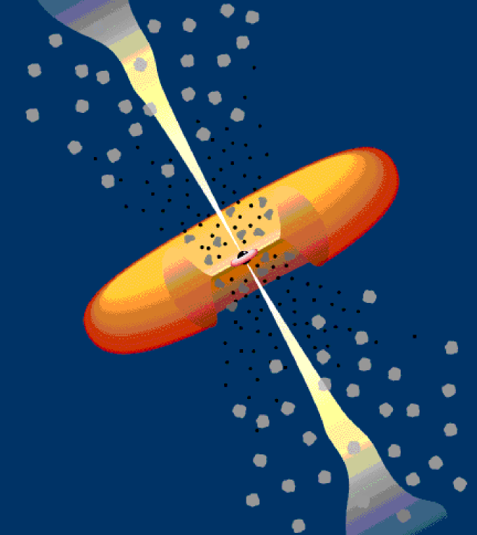
Figure 1.1: Schematic representation of an active nucleus.

Drawing on the spectroscopic classification of Seyferts, AGN generally are now classified ‘Type 1’ and ‘Type 2’. Type 2 objects are those with no evidence of a direct view of their central engines: radio galaxies exhibiting only narrow emission lines (NLRGs) join Seyfert 2s in this category. Type 1 objects are those which do seem to include radiation from the central engine, and Seyfert 1s are joined by BLRGs (broad-lined radio galaxies – which also show the narrow lines), and by quasars.

One important prediction of the Unification Model is that Type 2 objects, with their torus axis being aligned roughly in the plane of the sky, ought to include broad line regions (BLRs) whose light, though obscured from Earth, escapes into the plane of the sky. Dust particles or electrons in the host galaxy or in the clouds responsible for the narrow lines should scatter some of this light into our line of sight. When light becomes scattered, it becomes linearly polarized in the sense perpendicular to the pre- and post-scattering flight axes of the photon; hence linearly polarised imaging or spectroscopy of AGN should reveal light from BLRs polarised perpendicular to the direction of the radio jet (presumed to be aligned with the opening of the torus).

The motivation of this thesis is to search for evidence of such polarization in $K$-band infrared light from radio galaxies – a waveband thought, but not proven, to be dominated by light from the host galaxy’s stars rather than the active nucleus. Findings of $K$-band polarization would set important constraints on the relative strengths of the nuclear and stellar components. Accordingly, the next chapter presents a review of the status quo  in our knowledge of the relationship between radio galaxies’ radio structure and their morphological and polarization properties. First, however, we must look at the ‘big picture’ of the different classes of AGN known to exist, and how they might be related to one another if the best-buy Unification Hypothesis is correct.

1.2 The Unification Hypothesis for AGN

Contemporary authors embrace the Unification Model as the accepted model for AGN with various degrees of enthusiasm: Antonucci [1993] rushes to set it up as the ‘straw person model’ against which he reviews the current observational evidence; for Robson [1996, ch. 9] it is a solid foundation, while Peterson’s [1997, ch. 7] approach is more cautious. There is no other serious contender to explain the wide range of AGN phenomena, although in certain individual objects [1997, §§2.4, 3.4] starbursts rather than black hole accretion may form the hidden engine driving the radiation output.

A fundamental division between the various classes of AGN is their radio strength. Radio galaxies, by definition, are radio loud. Seyferts are empirically found to be radio quiet. All blazars, without known exception, are radio loud; 90–95% of quasars are radio quiet. The various classifications of AGN stem historically from the (often extreme) prototypes of each class first discovered, and are not always helpful in classifying less extreme examples: for instance, a radio-loud galaxy with an obvious active nucleus would now be classified a radio galaxy rather than a Seyfert, so the absence of radio-loud Seyferts is a consequence of taxonomy rather than physics. While some attempt has been made to define the different AGN classes more rigorously [1997, ch. 2], the older literature and human nature militate against the use of clear-cut terms to distinguish different classes of object – objects which are hypothesised to lie on a continuum of classes in any case!

1.2.1 Seyfert Galaxies

As summarised earlier, the first key to unification came from studies of Seyfert galaxy spectra. Seyferts are now defined as low luminosity AGN with absolute magnitudes $M_{B}>-21.5+\log h_{0}$ [1997, §2.1]; it follows naturally, therefore, that all known Seyferts are at low redshift and their morphology is open for study. Nearly all Seyfert AGN are found to lie within spiral galaxies [1997, §8.1.1], often of type Sa or Sb, and the host galaxies are more likely than normal spirals to be barred and/or deformed. Robson [1996, §3.2] notes that in the rare cases where Seyferts are radio-loud, they often have other peculiar characteristics.

Spectral studies of Seyferts led to the Type 1 / Type 2 classification based on the presence or absence of broad spectral lines. The discovery of broad lines in Type 2 Seyfert NGC 1068 in polarised light [1985] prompted the realization that the Broad Line emitting Region (BLR) must lie within some geometrical feature which screened it from direct view. This screening feature – the postulated molecular torus – is typically of diameter $\sim$ 100 pc, and should not be confused with the accretion disk in the central engine, measuring perhaps 0.03 pc. A typical schematic diagram is Figure 7.1 of Peterson [1997]; an excellent cartoon sketching the structure of an AGN at eight different scales ($10^{-4}$–$10^{+6}$ pc) is borrowed from Blandford by Robson [1996, Figure 9.9].

Recent studies of the near-infrared ($H$-band) polarization of NGC 1068 [1996, 1997] have been found to be consistent with a scattered light hypothesis and have even allowed the likely position and orientation of the molecular torus to be identified: the torus in this case has a diameter greater than 200 pc.

Miller & Goodrich [1990] studied eight further Seyfert 2s to see if spectropolarimetry would reveal Seyfert 1 features, choosing objects already known to have high broadband polarizations. Four gave definite positive results, two gave definite negatives, and two failed to produce reliable signal-to-noise. The four polarised galaxies revealed polarized features consistent with Seyfert 1 properties, albeit with a degree of ‘bluing’ in the spectrum indicative that dust scattering must be a contributing mechanism. Three of these, and possibly one of the two low signal-to-noise sources, exhibited perpendicular alignment between the polarization orientation and the radio axis. Similar perpendicular alignments had also been detected in Seyfert 2s by Antonucci [1983]. Weak parallel  polarizations have been observed in a few Seyfert 1s [1990, and references therein].

The nuclear polarization levels obtained by Miller & Goodrich [1990] were only of the order of a few percent — rather low if the underlying mechanism is the scattering implied by the perpendicular alignment. Antonucci [1993] speculates that they may have underestimated the contribution of host galaxy starlight, and that the true polarization may be closer to the 16% level observed in NGC 1068.

Further tests for the Unification Model in Seyferts are reviewed by Antonucci [1993] — some may indicate refinements that need to take account of additional parameters in the model (e.g. the opening angle of the molecular torus) but none fatally wound the principle of Unification. Claims that some Seyfert 2s contain no BLR emission [1993, §2.6.2] call for more sensitive spectropolarimetry before they can seriously question Unification: Robson [1996, §3.2] and Peterson [1997, §7.4.1] note that this is a hot area of current research. Until proven otherwise, it can be safely stated that Seyfert galaxies fall into two distinct classes: broad line (Type 1) objects which sometimes exhibit weak polarizations parallel to the radio structure, and narrow line (Type 2) objects which often display strong perpendicular polarizations.

1.2.2 Blazars

The precise definition of a blazar seems to depend on which source is consulted. I will follow Robson’s [1996, §3.6.4] helpful advice that the term refers to a phenomenon rather than a simple class of object: specifically, the phenomenon of a relativistic jet beamed roughly in the direction of terrestrial observers, dominating the radio thru infrared spectrum with its non-thermal synchrotron emission. The blazar phenomenon is exhibited by three classes of object: BL Lacertae objects (BLLs), optically violent variable sources (OVVs), and highly polarized quasars (HPQs).

BLLs are distinguished and defined by the lack of emission or absorption features in their spectra. They often exhibit variability (changing their output by several magnitudes in the space of a few weeks) and usually lie in elliptical galaxies, though spiral hosts are also known. OVVs are AGN (with spectra including broad emission lines) which exhibit short timescale luminosity variations ($\mathrel{\mathchoice{\vbox{\offinterlineskip\halign{\hfil$\reset@font\displaystyle#$\hfil\cr>\cr\sim\cr}}}{\vbox{\offinterlineskip\halign{\hfil$\reset@font\textstyle#$\hfil\cr>\cr\sim\cr}}}{\vbox{\offinterlineskip\halign{\hfil$\reset@font\scriptstyle#$\hfil\cr>\cr\sim\cr}}}{\vbox{\offinterlineskip\halign{\hfil$\reset@font\scriptscriptstyle#$\hfil\cr>\cr\sim\cr}}}}0.1$ mag) over timespans as short as a day [1994, 1997, §2.5]. No radio-quiet OVVs or BLLs are known [1993].

Antonucci [1993, §3.1] argues strongly that the distinction between BLLs and OVVs is ill-founded – especially given that the sources’ very variability can switch them between the two categories – and that in fact all radio-loud AGN with radio structures dominated by emission from the core are part of the same family of objects. The optical components of core-dominated radio-loud AGN tend to be quite red, highly variable, and polarized: this is proposed to be the high-frequency tail of the core synchrotron emission. Only emission from the core can vary coherently over timescales of weeks or days. He proposes that BLLs are simply the extreme cases where the synchrotron emission utterly dominates other components of the optical output, and predicts that more sensitive spectropolarimetry of BL Lacertae objects would reveal faint unpolarised broad emission lines from the BLR clouds basking in the synchrotron jets. Conversely, he also suggests that those core-dominated radio-loud AGN not classed as blazars would reveal a faint red optical core under careful scrutiny.

Robson [1996, §3.6.4] also includes HPQs in his phenomenological class of blazars. Scarpa & Falomo [1997] recently compared the optical properties of a sample of HPQs and BLLs, finding that optical properties of radio-selected BL Lacertae objects were very similar to those of highly polarised quasars. An earlier survey comparing high- and low-polarization quasars [1984] found that all but two of their HPQs were radio-loud, and the two radio-quiet quasars had their own peculiarities. The orientation angles of the HPQ linear polarizations seemed randomly distributed with respect to the radio axes; this bears out the core emission hypothesis, as the synchrotron mechanism produces light whose polarisation orientation has no relationship with the radio jet geometry. It seems eminently reasonable to accommodate HPQs between less extreme core-dominated radio-loud AGN and the OVVs on Antonucci’s unified blazar scheme.

1.2.3 Quasars

Complementing the definition of Seyferts, above, quasars are now defined as AGN with absolute magnitudes $M_{B}<-21.5+\log h_{0}$ [1997, §2.2]. A small proportion (5-10%) are known to be radio-loud; spectroscopically, quasars exhibit spectra similar to Type 1 Seyferts [1997, §7.4.1]. Since Moore & Stockman [1984] found HPQs to be quite distinct from low polarization quasars (LPQs) we have already dealt with HPQs as blazars; and Stockman, Moore & Angel [1984] undertook a specific study of the LPQs. The cut-off cannot be precisely defined, but 3% polarization is normally taken as an effective working threshold in the literature.

Stockman, Moore & Angel [1984] found that the typical LPQ polarization was around 0.6% and tended to be aligned parallel with the radio axis. There was no strong evidence for temporal variability in the degree or orientation of polarization, with upper limits of $\Delta p/p\leq 0.16$ and $\Delta\phi\leq 8\hbox{${}^{\circ}$}$. In a sub-sample of LPQs mostly selected in the radio, the $B$-band polarization was typically 50% greater than the $R$-band value; the equivalent test was not performed on optically-selected LPQs. The lack of variability and the tendency for polarization to increase at shorter wavelengths rules out a blazar origin for the polarized light in LPQs: models invoking scattering off dust grains or electrons in a disk or oblate cloud could account for such polarization but the mechanism is still very unclear. Stockman, Angel & Miley [1979], Antonucci [1982] and Moore & Stockman [1984] provide evidence for a bimodal (parallel/perpendicular) distribution of scattering angles; perpendicular alignments can be easily accounted for by the usual mechanism. Antonucci & Barvainis [1990] suggest that the parallel LPQs and the few Seyfert 1s that exhibit weak parallel polarization may contain disks or tori with very large opening angles, which could produce parallel polarization by scattering.

The Stockman, Moore & Angel [1984] survey covered bright objects from a variety of catalogues, and was not statistically complete in any meaningful sense. To complement it, Fugmann & Meisenheimer [1988] studied a sample of faint 5 GHz radio sources, and more recently, Impey, Lawrence & Tapia [1991] studied the optical polarization of a complete sample of radio sources, also selected at 5 GHz.

Impey, Lawrence & Tapia’s [1991] complete 5 GHz sample included both radio galaxies and quasars. Since HPQs are known to exhibit strong variability, it is possible that they may sometimes drop below the 3% threshold and are at risk of being labelled LPQs on the strength of a single measurement. Discovering a trend of polarization increasing with radio compactness, Impey, Lawrence & Tapia [1991] note that they ‘cannot exclude the possibility that all  quasars with compact radio emission have $p_{\mathrm{m}ax}>3\%$, at least some of the time’. Again, this would support a division of radio-loud quasars into those which are part of the blazar family, aligned such that their radio core would appear compact, and those whose beaming axis is not so closely aligned with the line of sight to Earth. Fugmann & Meisenheimer’s [1988] results also suggest that many compact radio objects not otherwise noted for optical variability exhibit polarization properties characteristic of blazars. Robson [1996, §3.4.1] notes that the polarization properties of radio-quiet quasars have not been well measured, but are tightly constrained in the optical as being very low — low enough to be attributed to thermal emission.

One unanswered question for the Unification Model is why Type 2 spectra are not seen in quasars. Peterson [1997, §7.4.1] offers two suggestions: that the molecular torus surrounding such a powerful central engine is thinned to the point of ineffectiveness; or that ‘Quasar 2s’ exist but have been misidentified as something else, perhaps the ultraluminous far infrared galaxies [1988].

Robson [1996, §9.2.3] pursues the latter hypothesis in the shape of IRAS galaxy IRAS FSC 10214+4724. This remarkable object, at $z=2.286$, appears to be gravitationally lensed, to be undergoing a starburst phase, and  to contain an active nucleus! Images [1993] taken through polarizing filters reveal a polarization of about 16% regardless of aperture, but ambiguous indications of any Alignment Effect. Polarized spectra [1996] reveal broad quasar-like emission lines. Dust scattering from an active nucleus is proposed as the most likely source of the polarization, but scattered light from a blanketed starburst might also provide an explanation. IRAS 09104+4109 [1993] is also notable as an IRAS galaxy containing a powerful radio source and with a constant nuclear polarization of $\sim 18\%$, although the polarization is misaligned with its radio structure (possibly due to the geometry of thin regions in its blanketing dust). Both Antonucci [1993] and Robson [1996, §9.2.3] speculate that future analyses of the most luminous IRAS galaxies will reveal some (perhaps ten percent) of them to be hiding the missing Type 2 quasars.

1.3 Radio Galaxies

Radio Galaxies form the remaining category of AGN. Most of the AGN sources considered so far have been radio-quiet, except for the blazars which are dominated by strongly beamed radiation over many decades of their spectrum. Radio galaxies join the 5-10% of quasars in the distinct class of radio-loud AGN. Reviewing the status of high redshift radio galaxies, McCarthy [1993] notes that the distinction between radio galaxies and radio quasars is becoming blurred as the host galaxies of quasars have been identified for quasars with $z\mathrel{\mathchoice{\vbox{\offinterlineskip\halign{\hfil$\reset@font\displaystyle#$\hfil\cr<\cr\sim\cr}}}{\vbox{\offinterlineskip\halign{\hfil$\reset@font\textstyle#$\hfil\cr<\cr\sim\cr}}}{\vbox{\offinterlineskip\halign{\hfil$\reset@font\scriptstyle#$\hfil\cr<\cr\sim\cr}}}{\vbox{\offinterlineskip\halign{\hfil$\reset@font\scriptscriptstyle#$\hfil\cr<\cr\sim\cr}}}}0.5$. Classically, the distinction had been that a powerful radio source was a ‘quasar’ if the host galaxy could not be seen beneath the active nucleus; an ‘N galaxy’ if the nucleus was exceptionally bright but did not wash out all traces of the starlight; or an ordinary radio galaxy otherwise.

1.3.1 The spectra of radio galaxies

Today, radio galaxies are classified on the basis of two distinct sets of properties: their optical emission lines and their radio structure. McCarthy [1993] notes that Broad Line Radio Galaxies (BLRGs), i.e. those with H i lines having widths over 2,000 km/s, tend to have the morphological classification of ‘N galaxies’, and their broad line spectra are similar to those exhibited by Seyfert 1s. Narrow Line Radio Galaxy (NLRG) spectra have only narrow lines for both permitted and forbidden transitions; BLRGs have narrow forbidden line spectra similar to those of NLRGs.

A distinction is often made between ‘nuclear’ and ‘extended’ emission, but isolating the nucleus from any extended emission region is not trivial when a 2^′′ slit encompasses more than 10 kpc of an object at $z>1$. If spectroscopy can be performed on distinct regions of a radio galaxy (an operation not possible with unresolved quasars), the properties of the spectra would enable the composition of the different parts of the galaxy to be identified. Similarly, imaging polarimetry has the potential to be an invaluable tool to determine the properties of different parts of the emission. But both techniques are limited in practice by the faintness of the galaxies [1996].

The optical radiation emitted by radio galaxies is thought to be a combination of starlight and nebular emission from the host galaxy, and a quasar-like (power-law) component originating in the active nucleus hidden in the heart of the galaxy. [Note that at this stage we need make no assumptions about the reason  for the shape of the quasar spectrum, but only utilise its profile. It has been suggested [1988] that the quasar spectrum could be synthesised from a suitable combination of blackbody curves.]

Manzini & di Serego Alighieri [1996] tested this three-component hypothesis by modelling radio galaxy spectra at rest frame wavelengths from 0.2 m to 1.0 m. Starlight from the host galaxy was modelled as the synthetic spectrum of Bruzual & Charlot [1993] for a galaxy with an initial burst of star formation and no subsequent formation. Nebular emission was modelled with a spectrum selected from Aller [1987]. The active nuclear component was modelled by the composite radio-loud quasar spectrum of Cristiani & Vio [1990], and attenuated according to different distributions of dust grains which might be present to scatter nuclear light into the line of sight to Earth.

Manzini & di Serego Alighieri [1996] applied their modelling to a small sample of radio galaxies at redshifts ranging from 0.11 to 2.63, and have demonstrated that their observed magnitudes (by multiwaveband photometry) are consistent with artificial spectra synthesised from three such components. The contribution of the starlight becomes greater to longer wavelengths, while the nuclear component decreases. For five out of their six galaxies, the stellar component of the light has become dominant by a rest-frame wavelength of 0.5 m; in 3C 277.2 $(z=0.766)$ the starlight only exceeds the nuclear component at about 0.85 m. Hence the ‘galaxy plus quasar’ model predicts that starlight should dominate the infrared output of radio galaxies, while nuclear emission is predominant in the ultraviolet. Hammer, LeFèvre & Angonin [1993] confirm that the ultraviolet $\lambda<400$ nm light from $z\sim 1$ 3C radio galaxies is dominated by the presence of an active nucleus.

We have already noted (§1.2.1) that the distinction between BLRGs and NLRGs can be interpreted as a Type 1 / Type 2 orientation effect, with the BLR obscured by an assumed molecular torus in those galaxies classed NLRGs. Quasars and radio galaxies have been shown to have comparable emission line luminosities, arising in emission line regions less than 1 kpc in diameter [1982]. If the Unification Model is the correct model to apply to radio galaxies, then Manzini & di Serego Alighieri [1996] are correct to model their ‘quasar’ component as scattered into the line of sight by dust; and their results show that radio galaxies can be accurately modelled as containing quasar cores (with molecular tori of dimensions less than 1 kpc), with core light scattered by plausible (albeit idealized) distributions of dust.

1.3.2 The Hubble diagram: radio galaxy evolution

If the infrared emission of radio galaxies is dominated by starlight, then studies of the variation of their $K$-band magnitudes with redshift should tell us something about galactic evolution. Lilly & Longair [1984] produced a $K-z$ plot, or Hubble diagram, for 3CR radio galaxies, i.e. for those radio galaxies with the most powerful radio emissions. Two features were evident in the resulting Hubble diagram: the dispersion of the $K$-magnitudes about the average value remained constant up to $z\mathrel{\mathchoice{\vbox{\offinterlineskip\halign{\hfil$\reset@font\displaystyle#$\hfil\cr>\cr\sim\cr}}}{\vbox{\offinterlineskip\halign{\hfil$\reset@font\textstyle#$\hfil\cr>\cr\sim\cr}}}{\vbox{\offinterlineskip\halign{\hfil$\reset@font\scriptstyle#$\hfil\cr>\cr\sim\cr}}}{\vbox{\offinterlineskip\halign{\hfil$\reset@font\scriptscriptstyle#$\hfil\cr>\cr\sim\cr}}}}1$, but the average magnitude evolved with redshift such that galaxies at $z\sim 1$ were about 1 mag more luminous than at $z=0$.

Eales & Rawlings [1996] summarise the natural interpretation of these findings: low dispersion implies that the radio galaxies were not passing through any transient phase in their evolution (which would have caused wider variation in their luminosity) over the span of redshifts covered. The declining luminosity to lower redshifts is consistent with a period of star formation at $z>5$, followed by passive evolution as stars of decreasing mass reach the end of their lives. This seems perfectly reasonable since nearby radio galaxies are known to lie within giant ellipticals with a small spread of absolute magnitude [1983], and a similar evolutionary model has been suggested for radio-quiet elliptical galaxies [1962]. Imaging of the rest-frame visible structure of radio galaxies out to $z\sim 2$ shows many of them to have dynamically relaxed structures, suggesting that these are active elliptical galaxies, too [1992, 1992, 1994].

It should be noted, however, that many distant radio galaxies at $z>0.6$ [1993, 1994, see below] do not have elliptical morphologies: an evolving elliptical model alone cannot explain the disturbed morphology of these objects, so at best a modified evolving elliptical model is needed. [It has also been suggested that the radio galaxies are in fact young objects which pass through a radio-loud phase only a few hundred Myr after a rapid star-forming phase itself lasting of order 100 Myr [1990].]

Lilly & Longair’s [1984] Hubble diagram suffers from the unavoidable selection effect that 3CR galaxies contain the most powerful radio sources. Eales et al. [1997] therefore analysed a 90% complete set of radio galaxies selected at lower radio luminosities in the B2 and 6C catalogues, and created a Hubble diagram allowing the $K$-magnitudes of 3CR galaxies to be compared to those whose radio output was only one-sixth as strong. Analyzing the diagram above and below the natural threshold of $z=0.6$, they found that the low redshift B2/6C galaxies had $K$-magnitudes statistically identical to the 3CR sample, but at $0.6<z<1.8$, the 3CR sample was brighter by a median 0.6 magnitudes. Demonstrating that sources of bias have either been eliminated or would make their result stronger, Eales et al. [1997] argue that the $K$-band emission of the brightest radio galaxies must be contaminated by light from a source whose luminosity is correlated with the radio strength of the galaxy – presumably direct or indirect $K$-band emission from the active nucleus itself (but see below).

Eales & Rawlings [1996] note that Hubble diagram for the 6C/B2 galaxies (assumed to be unpolluted by nuclear emission) follows a curve for no  stellar evolution; the 3C Hubble diagram which had previously been interpreted as indicating stellar evolution rather represents a series of galaxies showing no evolutionary effects, hosting nuclear sources which tend to be brighter at higher redshift by the selection effect of a flux-limited radio sample. It has been argued [1998] that the apparent ‘no evolution’ result occurs because of a cosmic conspiracy: the host galaxies of the radio sources evolve in the same way as radio-quiet Brightest Cluster Galaxies (BCGs). The $K-z$ Hubble diagram for BCGs also suggests an unphysical no-evolution scenario, which must be accounted for by postulating evolution in the galactic structure whose net effect counteracts that of stellar evolution. The most likely explanation is ongoing formation according to hierarchical clustering models. Radio galaxies are preferentially found in clusters at high redshift, so it would not be surprising for their behaviour to follow that of BCGs; while the fact that low-redshift radio galaxies are not preferentially found in clusters should make us suspicious of accepting Lilly & Longair’s [1984] continuous Hubble diagram across the $z=0.6$ morphology break.

Best, Longair & Röttgering [1998] argue that $K$-band emission from the active nucleus cannot contribute more than 15% (typically 4%) to the brightness of a 3CR radio galaxy, nor cause more than 0.3 mag of brightening in 3CR objects over 6C objects. Ruling out the possibility that 3CR objects contain more young stars, they suggest rather that 3CR objects simply contain greater masses of stars, and cite evidence [1995] that if the central engine is a black hole whose accretion rate depends on the material available in the host galaxy, then the mass of stars in the galaxy will be correlated with the radio, and hence the optical [1998, 1998].

1.3.3 The radio morphology of radio-loud AGN

The radio classification of radio-loud AGN distinguishes those which are ‘lobe-dominated’ and those which are ‘core-dominated’ [1996, §3.7]. A more detailed discussion of the different radio structures observed in radio galaxies is given by Miley [1980, §2.1].

Measurements of radio flux density, $S$, at different frequencies allow a power law spectrum to be fitted to the source, characterised by a spectral index $\alpha$, such that $S\propto\nu^{-\alpha}$. Core-dominated radio sources tend to have flat spectra ($\alpha\sim 0$) and often show a single kpc-scale jet; in fact, most core-dominated radio sources would fall into the category of blazars rather than radio galaxies [1996, §3.7.2] — and there is recent evidence that radio galaxies which are core-dominated exhibit variable optical polarization due to synchrotron emission [1997, 1998].

Lobe-dominated radio structures emit radio waves from a locus of space which can span many tens of kiloparsecs, up to 3 Mpc in the case of 3C 236 [1996, §3.7.1]. The extended lobes of radiation are zones of synchrotron emission, and are fed by a stream of relativistic electrons flowing out of the poles of the central engine. The radio spectra of lobe-dominated sources tend to be steep, with $\alpha\sim 1$.

A further division is made according to the criteria of Fanaroff & Riley [1974], whence sources with spectral luminosity density $P_{\mathrm{1}78\,MHz}>5\times 10^{25}$ W Hz^-1 are class FR II, and those less luminous are class FR I. The class FR I sources are usually associated with radio galaxies alone, and the most prominent parts of the the radio structure (‘hot spots’) lie closer to the core than to the edge of the radio structure.

Both quasars and radio galaxies can exhibit class FR II structure, and their hotspots lie closer to the edge of the emission region than to the core [1994]. Such sources usually have a compact radio core co-located with the optical nucleus of the galaxy. All radio-loud quasars and many class FR II radio galaxies are asymmetric, with a kpc-scale jet only visible between the core and one of the lobes [1996, §8.1]. The most likely explanation of the asymmetry again invokes an orientation argument, with those jets travelling towards us closest to our line of sight being most Doppler-brightened and the counterjets similarly Doppler-supressed [1996, §8.2.1]; hence quasars, where we are thought to be looking close to ‘down the jet’, are always asymmetric, while radio galaxies are viewed closer to ‘sideways on’ and the two jets can appear to be of comparable brightness. This has been borne out by the discovery of the Laing-Garrington effect [1993, §3.4], where the radio emission from the far side of such a source suffers depolarization by its passage through the interstellar material in the host galaxy and hence appears less polarized than the radio emission from the lobe associated with the jet.

For nearby radio galaxies, class FR II sources are normally found in (otherwise normal) giant elliptical galaxies, although not in galaxies forming part of rich clusters. Nearby FR I sources, however, are very likely to be hosted by more luminous ellipticals, often the type D or cD galaxies which dominate rich clusters [1996, §3.7.1]. At high redshift, though, there is no clear evidence for a distinction between the richness of clusters hosting FR I and FR II classes; and the morphology of the host galaxy is often distorted by the presence of knots. We will return to this in the next chapter, in a discussion of the Alignment Effect.

1.3.4 Radio source unification revisited

The presence or absence of strong radio emission seems to be a fundamental characteristic of AGN, and is strongly linked with optical morphology: Peterson [1997, §8.1.3] notes that it is ‘true in general’ that radio-quiet AGN (Seyferts, most quasars) are found in spiral galaxies [but see Ridgway & Stockton [1997] and references therein for evidence of elliptical hosts being common in radio-quiet quasars], while strong radio sources (radio quasars, radio galaxies and blazars) tend to have elliptical hosts. Further, the host galaxies of radio quasars are, on average, 0.7 mag brighter in absolute $B$-magnitude than radio-quiet quasar hosts. The absence of FR I class quasars may follow from the strength of the central engine: if the nucleus is powerful enough to be optically classified a quasar, then its jets may de facto  be strong enough to produce FR II class radio structure.

The first indications that orientation effects may be important in understanding the nature of radio sources came with the discovery of apparent superluminal motion in four of the brightest radio sources [1977]. Superluminal observations can be understood if the source is ejecting matter at relativistic velocities along a path close to the line of sight to the observer [1966, 1979]; in which case superluminal sources must be the beamed subset of some parent population. This model is now generally accepted as the explanation of superluminal radio sources and is consistent with other observed features of the superluminal sources – including blazar properties and asymmetric jets [1989].

The Unification Model predicts that radio galaxies should not exhibit superluminal motion. Of Cohen et al.’s [1977] four original superluminal sources, three were quasars but the fourth was classed as a radio galaxy. This object, 3C 120, is a nearby $(z=0.033)$ galaxy which has been variously classified as a core-dominated broad-line radio galaxy, and as a radio-loud Seyfert 1 with disturbed morphology [1997]. If we set aside 3C 120 as an anomalous object, what of other AGN? A survey of relativistic motion in all sources of known VLBI core size, appearing in the literature 1986–1992, was assembled by Ghisellini et al. [1993]. Of the sources for which speeds were recorded, definite superluminal velocities were observed in all 11 BLLs, 23 out of 29 quasars (with 5 more having superluminal upper limits), and none of 6 radio galaxies. One radio galaxy (0108+388) displayed an apparent speed of $1.0c$, and another (0710+439) had an upper limit of $2.5c$ quoted. Neither of these findings are strong enough to prove the existence of superluminal motion in a radio galaxy.

The Unification Model hypothesises that radio-loud quasars are an oriented subset of some intrinsically radio-loud parent population. Barthel [1989] poses the question, ‘Is every quasar beamed?’, and reviews the evidence. As discussed above, those quasars which show superluminal motion are likely to be beamed, and we have also considered the evidence of the Laing-Garrington effect. A beaming hypothesis can explain several statistical properties, including the correlation between brightness and component motion, and more limited statistics showing that lobe-dominated sources display lower superluminal velocities than core-dominated (more closely aligned?) sources. Against that must be set the problem of why certain radio-loud quasars have very large extended structures, whose deprojected linear size would be enormous; and the statistical finding that the asymmetric brightness of jets over counterjets is, on average, larger than can be accounted for by beaming effects alone if the parent population is of randomly oriented quasars.

Barthel [1989] goes on to demonstrate that by assuming the parent population is of powerful radio galaxies, with quasars as the beamed subset, the statistics of jet/counterjet asymmetries can be justified; and the sizes of the largest radio galaxies are such that the largest superluminal quasars are not too large in the context of the parent population. Radio-loud quasars and FR II radio galaxies at $0.5<z<1$ in the 3CRR catalogue were compared; after the exclusion of unsuitable candidates, 12 quasars and 30 radio galaxies remained, with the linear dimensions of the galaxy radio structure averaging about twice that of the quasar mean. The relative numbers suggest that a source will appear as a quasar if viewed within $44.4\hbox{${}^{\circ}$}$ of its axis, and as a radio galaxy otherwise. This being the case, the quasars should be foreshortened 1.8 times as much as the radio galaxies, consistent with the observed factor of 2. [If the radio-quiet unbeamed counterparts of the quasars really are the far infrared galaxies, Barthel [1989] notes that the number count statistics are consistent with such unification: there are 11 quasars for every 49 far infrared galaxies.]

Further evidence for radio galaxy / radio quasar Unification comes from other wavebands [1989]: Blazars and quasars are known to be strong in their X-ray emission, while radio galaxies are weak; Seyfert 1s are luminous in X-rays while Seyfert 2s are not, suggesting that the molecular torus is an effective shield of X-ray radiation. On the other hand, the torus viewed from any angle ought to be bright in the far infrared because of its own heat, and detection statistics of both radio galaxies and quasars in this waveband bear this out. Two pieces of evidence oppose Unification, however: claims that the host galaxies of radio quasars differ significantly from radio galaxies [1987]; and that extended radio sources lie in denser environments than compact sources [1988].

Robson and Antonucci draw differing conclusions on how blazars fit into the unification picture. We have already seen how Antonucci [1993, §3.1] proposes that BLLs and OVVs are attributed to different luminosities in otherwise similar synchrotron cores. Recall that under this scheme, BLLs are postulated to be blazars with the most powerful synchrotron sources, whose emission effectively drowns out the broad lines from the BLR which lies in the line of sight. Robson [1996, §8.4.2] suggests that BL Lac objects are not end-on quasars, claiming rather than BLLs are beamed FR I objects and OVVs are beamed FR II objects — and noting differences in the radio polarization properties of BLLs and OVVs which hint that BLLs are more likely to have shocks in their jets. The absence of emission lines in BLLs would be related to the weakness of the output of the line-emitting clouds rather than the overpowering strength of the optical synchrotron core emission. Ghisellini et al. [1993] find that their statistics from a survey of 105 radio-loud AGN support this idea.

Antonucci [1993, §3.1] warns against the automatic identification of the BLL/OVV classification with the Fanaroff-Riley class, noting that some famous BL Lacs are FR class II [1992]. What is clear, is that many blazars have sufficient radio output in their diffuse emission alone to make it into the 3C or 4C catalogues; and so ‘misaligned blazars’ not beamed towards the Earth must be part of a unified continuum with some other classes of AGN which are already known.

One modification to the standard Unification Model is that some putative radio galaxies may be quasars obscured not by their molecular torus, but by other obscuring material. For instance, infrared spectroscopy revealed a broad H$\alpha$ line in ‘NLRG’ 3C 22 [1995], suggesting that this source may be in the quasar orientation, but with opaque material obscuring much of the light from the active nucleus. Similarly polarization measurements of 3C 109 [1992] can be understood if there is a hidden quasar core whose light suffers polarization by transmission through dust. If such obscured quasars are common [1998, 3C 234 could be another example], then many putative radio galaxies may have their axis closer to their line of sight to Earth than hitherto thought, and orientation statistics will be affected accordingly.

Two major questions remained unanswered by current Unification models. Why do some galaxies and quasars produce jets strong enough to drive radio emission, and others not? Why is radio emission is only found in elliptical galaxies? We shall not pursue these questions or debate the nature of blazars here, as such matters lie outside the scope of this thesis, but pause to note that work is still very much in progress on the refining of the Unification Model.

Chapter 2 The Alignment Effect and Polarization in Radio Galaxies

There comes a time when for every addition of knowledge you forget something that you knew before. It is of the highest importance, therefore, not to have useless facts elbowing out the useful ones.
— Sherlock Holmes, A Study in Scarlet.

The current paradigm within which radio galaxies are explored is that of the Unification Hypothesis. We have already explored how this hypothesis can be used to account for the wide range of AGN phenomena described in the previous chapter; now we look more specifically at radio galaxies. Distinctively among AGN, radio galaxies often display significant alignments between their radio structures and the orientation of their polarization and/or optical structure. Study of these alignments can help confirm or refute the appropriateness of the Unification Hypothesis to describe individual radio galaxies, and statistically, the class as a whole.

2.1 Polarization in AGN

Since active nuclei lie within host galaxies whose stars emit unpolarized blackbody radiation, the measured polarization of any active galaxy will be that of the active nucleus diluted by starlight. It is important to distinguish whether polarization figures quoted in a given case are those of the raw measurement, or corrected for removing the unpolarized stellar intensity to yield the polarization of the nucleus. The contribution of starlight diminishes in the near ultraviolet and at shorter wavelengths; rest-frame ultraviolet measurements can be presumed to give a good indication of the nuclear polarization.

The 1980 review paper of Angel & Stockman summarised what was then known of the visible and infrared polarization of extragalactic objects: the three classes of active galaxies known to produce polarised light were blazars, quasars and Seyfert 2s. Although the spectra of BLRGs suggested that they were related to quasars and Seyfert 2s, their relative faintness meant that polarimetric studies of low redshift radio galaxies did not appear in the literature until the early 1980s [1982, 1983], and high redshift studies a decade later [1993].

Angel & Stockman [1980, §IV] wrote before the Unification Hypothesis had become popular, and reviewed numerous mechanisms which might account for the low visible/infrared polarizations observed in many Seyferts. Originally, Seyfert polarizations (of order 1%) were attributed to the visible high-frequency tail of synchrotron radiation. Multicolour and spectroscopic studies of Seyfert polarization, however, showed that in most Seyferts, both the core continuum light and the emission lines were polarised, and the polarization (corrected for the stellar contribution) was stronger in the blue than in the red, but with little rotation of position angle. These facts suggested that the total light emerging from the central engine was being polarised by some subsequent interaction, most probably with dust. [We dealt with this in some detail in §1.2.1.]

The discovery of Type 1 features in the polarised spectra of Seyfert 2s was the key to the first stage of Unification [1997, §7.1], the realization that orientation alone might be the distinguishing feature between the two classes of Seyferts. Antonucci’s [1993] review paper describes how the prototypical Seyfert NGC 1068 was investigated and found to be generating visible/ultraviolet light polarised at 16% in its nucleus. Since electrons scatter light equally strongly at all wavelengths whereas dust (via Rayleigh scattering and similar mechanisms) preferentially scatters blue light, it is implied that the scattering medium in NGC 1068 may be free electrons. Other Seyferts show evidence of higher nuclear polarizations at shorter wavelengths, characteristic of dust. Most yield a polarization orientation perpendicular to the radio structure, as would be expected for scattering.

Similarly, by the time of Antonucci’s [1993] paper, evidence was accumulating that BLRGs and NLRGs were the Type 1 and Type 2 classes for radio galaxies analogous to the classification of Seyferts. The picture seemed to be clearest for radio galaxies at redshifts $z>0.6$, where light measured in the $V$-filter on Earth corresponded to rest frame ultraviolet ($\lambda<330$ nm) emissions in the AGN, uncontaminated by significant starlight. The first measured high redshift radio galaxy polarization was reported in Nature  by di Serego Alighieri et al. [1989]; and since then, mounting evidence [1991, 1992, 1993, 1997] has generally borne out the empirical rule of thumb [1993] that distant radio galaxies $(z\mathrel{\mathchoice{\vbox{\offinterlineskip\halign{\hfil$\reset@font\displaystyle#$\hfil\cr>\cr\sim\cr}}}{\vbox{\offinterlineskip\halign{\hfil$\reset@font\textstyle#$\hfil\cr>\cr\sim\cr}}}{\vbox{\offinterlineskip\halign{\hfil$\reset@font\scriptstyle#$\hfil\cr>\cr\sim\cr}}}{\vbox{\offinterlineskip\halign{\hfil$\reset@font\scriptscriptstyle#$\hfil\cr>\cr\sim\cr}}}}0.6)$ should display diluted polarizations of 5% or more, oriented roughly perpendicular to the radio lobe structure.

In addition to this polarimetric evidence (reviewed in more detail below, §2.3.2), the apparent alignment of the knotted optical structures of high redshift radio galaxies with the radio axes [1987, 1987a, 1993, §5] lent weight to the concept of the torus and central engine proposed by the Unification Model. As we shall see in §2.3.1, this so-called ‘Alignment Effect’ is manifested most strongly in the AGN with the most powerful radio emission, and is intimately linked to the Unification Model and the presumed scattering mechanism for polarization.

While not proven – and inevitably suffering from a number of pathological cases which fit poorly – the Unification Model is now generally accepted, to the extent of being the foundation of the first textbooks on AGN to become available [1996, 1997]. The model must stand or fall, however, according to objective tests, not by indications of its popularity among astronomers. As new technology becomes available to the astronomical community, it is naturally the Unification Model which experiments are designed to test, and reinforce or falsify. With the recent availability of infrared arrays and polarisers [1997], it has become possible to extend imaging polarimetry into the $K$-band. The work contained in this thesis represents the first studies of linear polarization in high redshift radio galaxies in this waveband.

2.2 The Observational Challenge of Distant Radio Galaxies

2.2.1 Observational techniques

Modern astronomical detectors [1997] make a range of observational techniques available. Light from distant objects can be imaged on a detector array, and the light intensity measured in a synthetic aperture covering any part of the image. The light can be dispersed to form a spectrum or passed through an analyser which separates orthogonally polarised components.

Both spectroscopy and polarimetry are time-consuming procedures for faint objects: the former disperses the minimal available light into its component wavelengths, and the latter requires an accurate measurement of the intensity difference between the two orthogonal components of the light. Only recently has technology made it possible to employ both techniques simultaneously and perform spectropolarimetry of high-redshift radio galaxies, and our capabilities are limited: even with the light-gathering capacity of the 10 m Keck telescope, the resulting spectra must be rebinned at low resolution to extract a meaningful signal [1996]. Alternatively, if the orientation of the polarization is already known, a 4 m class telescope can obtain a spectrum of light polarized in the known direction in a reasonable time [1994].

The unique value of spectropolarimetry lies in its ability to identify the spectrum of scattered light present in the total signal, and so trace the emission properties of whatever hidden component is illuminating the scattering medium. (The spectrum will also, of course, give us an indication of whether polarization is attributable to a mechanism other than scattering.)

Images taken through a polarizing filter have their own value; photopolarimetry (i.e. photometry of polarized light) can be performed in synthetic apertures, yielding a polarization map or a study of the polarization of individual structures in an object of complex morphology. But again, the faintest sources are not amenable to a pixel-by-pixel polarimetric analysis; regions several pixels square may need to be binned together to obtain an acceptable signal-to-noise; and many of the radio galaxy figures given in the literature are simply polarizations integrated over the whole structure.

Where photopolarimetry is available in multiple wavebands, models of the polarized spectra of radio galaxies can be fitted against these broadband measurements: Manzini & di Serego Alighieri [1996] used this technique to establish their result (§1.3.1) that if the radio galaxies sampled consist of stars, nebular emission and an excess component in the form of a power-law, then starlight is still their dominant component in the near infrared.

2.2.2 The importance of the $K$-band

While observations of the rest frame ultraviolet have been important in polarimetric studies of AGN, on the assumption that the host galaxy contribution to the ultraviolet emission is negligible, the infrared is important for the opposite reason. Radio galaxies, as a species of AGN distinguished by their radio properties but [ideally] unremarkable in their optical emission, could be used as examples of ‘normal’ galaxies at high redshift (hence having experienced less cosmological evolution than nearby galaxies). They could be detected at high redshifts by virtue of their radio emission, and then studied optically in the hope that the active nucleus has not had too great an influence on their evolution (compared to ‘inactive’ galaxies), and is not polluting the light from the host galaxy. At high redshifts, of course, light originating in the visible or near infrared arrives at the Earth shifted into longer infrared wavelengths.

The atmospheric $K$-band window lies at a convenient wavelength for studying the near infrared properties of objects at $z\sim 1$, and the previous chapter reviewed how the $K-z$ Hubble diagram for 3CR radio galaxies [1984] suggested that the observed $K$-band light was essentially stellar emission from passively evolving elliptical galaxies. So in the late 1980s, $K$-band studies of radio galaxies were thought to be revealing the properties of young elliptical galaxies. As we have seen (§1.3.2), this has now been called into question by studies of fainter radio sources [1997]; and it seems that a substantial fraction of the observed $K$-band light in 3CR galaxies must come from the active nucleus after all.

While the Hubble diagram is a useful tool to analyse the statistical properties of a set of galaxies, it tells us nothing about individual galaxies. Studies of the polarization, morphology and spectra of 3CR galaxies are needed to determine the properties of their $K$-band excess; an understanding of the influence of the excess in individual radio galaxies is essential if we are to salvage their role as probes of galactic evolution.

The new observations presented in this thesis are polarized $K$-band images of nine radio galaxies, including seven from the 3CR catalogue. The signal-to-noise limit prevents the meaningful analysis of any structure finer than lobes of individual bright objects. In some cases, polarimetry in other optical bands is available and can be used together with our findings for comparison with synthetic spectra. In all cases, an upper limit can be assigned to the maximum contribution of any scattered component to the $K$-band light, providing an independent means of determining the influence of the active nucleus on the apparent luminosity of 3CR sources.

In the light of our measurements, and those in the literature, it is then possible to model the most likely mechanism giving rise to the observed polarizations. If the strength of the $K$-band emission is related to the power output of the central engine, the simplest explanation of this result is that a significant fraction of a radio galaxy’s infrared light emerges from the active nucleus in a restricted cone, and enters our line of sight after scattering by dust or electrons. In this case, as for the visible and ultraviolet light, the scattered infrared light should be polarised perpendicular to the direction of the radio jet. As we shall see in the rest of this chapter, the relationship between the polarization and structure of radio galaxies measured at radio, visible and infrared wavelengths is already well documented, and we shall discuss the properties of our representative sample of radio galaxies in this context.

The motivation for performing studies of the $K$-band polarizations of high redshift radio galaxies, therefore, is to probe the origin of their $K$-band emission. A finding of no polarization would suggest that infrared light could be used as a safe indicator of the properties of the host galaxy (but would make it hard to explain the suspected infrared Alignment Effect). A finding of infrared light polarised perpendicular to the radio axis would suggest scattered nuclear light; and where polarimetry exists in other wavebands, would provide a longer baseline to test the likely origin of the polarisation — electron scattering, dust scattering and direct sight of a synchrotron source each have a distinct dependence on wavelength. Any other finding would be an invitation to further scientific study!

2.2.3 The need for rigorous statistics

As in any scientific investigation, a thorough error analysis is required to give the final data their due weight. Polarimetry, however, is more demanding than other forms of photometry. Measuring a polarization is akin to determining the magnitude of a vector, a definite positive quantity. While the measurements of the vector’s components may fluctuate about zero for an unpolarised object, the magnitude stubbornly remains greater than zero and must be ‘debiased’ accordingly.

The astronomical literature contains not a few papers by statisticians [1985] and careful polarimetrists accusing astronomers of failing to debias their work adequately, although most 1990s papers on radio galaxy polarizations do address this issue. Given the need for debiasing polarization figures and the low signal-to-noise inevitable when studying objects at high redshift, a great deal of work in this thesis has been devoted to the accurate debiasing and error estimation of the data available. Much of the work has been published in the form of a step-by-step guide to polarimetry [1998]; the format has been retained, though the work has been refined and updated, in Chapter 3 of this thesis.

2.3 Observational Evidence for Orientation Correlations in Radio Galaxies

2.3.1 Evidence for the Alignment Effect

CCD technology of the mid-1980s allowed the optical structures of high redshift radio galaxies to be investigated for the first time. Radio galaxies at $z\sim 1$ were found to look nothing like the giant ellipticals associated with lower redshift radio galaxies; rather, the high redshift galaxies were often elongated and contained two or more bright ‘knots’ rather than a single identifiable nucleus [1984, 1984a, 1984b, 1987b]. After further studies of the most powerful radio sources, it was found that the major axis of the optical elongated or knotted structures was usually aligned within a few tens of degrees of the radio axis [1987, 1987a] – an association which has become known as the ‘Alignment Effect’.

Subsequent investigations with detectors sensitive to visible light revealed that the Alignment Effect cuts in at redshifts $z\geq 0.6$ [1993], and that the knotted optical structures are known to be emitting continuum  radiation, ruling out theories that the aligned structures are attributable to line-emitting gas clouds. More recent observations [1995, 1997, 1997] confirm the alignment of the rest-frame ultraviolet emitting regions with the radio structure.

There is no consensus at present about the mechanism which gives rise to the knotted structure; current observations continue to investigate the extent to which the Alignment Effect is associated with emission from the active nucleus. Two key tests of the relationship with the nuclear emission are whether the effect becomes weaker to longer wavelengths, and whether it becomes less prominent in less powerful radio galaxies.

The $z=0.6$ cut-off suggests that either there is an evolutionary process at work, or that we are observing a property of the rest-frame ultraviolet which does not extend to the rest-frame visible. Infrared observations of twenty 1 Jy galaxies at $z>1.5$ [1993] show little evidence for extended structure at rest-frame visible wavelengths. Conversely, $U$-band images of the low-redshift $(z=0.1)$ radio galaxy 3C 195 reveal a distinct aligned ultraviolet structure [1995], and a bipolar aligned structure is also seen in ultraviolet images of Cygnus A [1999]. Recent $U$-band imaging of the nearby radio galaxy NGC 6251 [1997] has revealed several extended regions of emission: the most prominent feature of this radiation lies interior to a dust ring, is nearly perpendicular  to the radio jet axis, and has a polarization below 10%.

The first $U$-band survey of low redshift radio galaxies (15 3CR objects at $0<z<0.6$) [1999] found evidence for $\Delta\phi<12\hbox{${}^{\circ}$}$ alignment between the radio axis and the $U$-band structure in 6 objects (two such alignments would be expected by chance alone). Two different mechanisms seemed to be at work: three sources showed alignment in the optical structure surrounding the radio nucleus, while the other three appeared to have a merging companion galaxy close to the radio axis. Of the three sources with an elongated nucleus, 3C 348 was also elongated in $V$ but gave no evidence for knots in either band, while the other two examples displayed knots in $U$ but no elongation or knots in $V$. The most radio-luminous radio galaxies, therefore, including those with no obvious aligned structure in the $V$-band, are now known to be able to display alignment in their near-ultraviolet structure at low redshifts, too.

The first $K$-band images of 3CR galaxies [1988, 1990, 1990] revealed that the near-infrared emissions of the most luminous radio galaxies displayed structure as knotted and complex as the ultraviolet emissions. As with visible light detectors, efforts were made to obtain infrared images of radio galaxies with lower radio luminosity. Many of these programmes used the $K$-band, in which observations of radio galaxies at $z\sim 1$ trace emissions at $\lambda\sim 1.1$ m in the rest frame.

Dunlop & Peacock [1993] compared $K$-band images of 3CR and PSR (Parkes Selected Regions) radio galaxies in a narrow bin of redshifts. The 3CR galaxies were selected at $0.8<z<1.3$, and the PSR galaxies ($S_{\mathrm{2}.7\,GHz}>0.1$ Jy) were known or estimated to be in a similar redshift range. A definite infrared-radio alignment effect was determined in the sample of 19 3CR galaxies, although the $K$-band structure was, on average, less extended than the optical structure. In some cases, the infrared structure seemed to be significantly more closely aligned with the radio axis than structure observed at visible wavelengths. These findings are consistent with the smaller 3C sample of Rigler et al. [1992], which suggested that an infrared alignment effect was present, but weak. Best, Longair & Röttgering [1997] imaged 28 3CR galaxies at $0.6<z<1.2$ and again found distinct alignments at visible wavelengths, with less complex structure and a weaker Alignment Effect in the infrared. On average, only about 10% of the $K$-band flux of 3CR galaxies at $z\sim 1$ is associated with aligned structures [1992, 1998].

Lacy et al. [1999b] investigated the Alignment Effect in a sample of $0.5<z<0.82$ 7C radio galaxies, with radio luminosities of order one-twentieth those of 3C galaxies. The Effect was still present, albeit very weakly above 400 nm, but only over small scales. 3C radio galaxies exhibit alignment in structures of order 15 kpc and 50 kpc; in the 7C sample, the effect seen at 15 kpc did not extend to structure at 50 kpc. Dunlop & Peacock’s [1993] PSR sample was tested in the $K$, $J$, $B$ and $R$-bands, with no evidence for alignment being found in the red or infrared, and only a possible marginal effect in the $B$-band. Wieringa & Katgert [1992] also found that the optical morphology of less luminous radio galaxies was more rounded.

Eales et al. [1997] criticise Dunlop & Peacock’s [1993] selection technique for the PSR galaxies: given that nuclear light biases upwards the apparent brightness of 3CR galaxies, the $K-z$ relation for 3CR galaxies cannot be used to estimate redshifts for PSR galaxies unless a correction is made for the nuclear component of the brightness. Constructing their own sample of 6C/B2 galaxies at redshifts well matched to Dunlop & Peacock’s [1993] 3CR sample, and following the same position angle analysis technique, Eales et al. [1997] found no strong evidence of an Alignment Effect, but a limited statistical analysis showed a probability $<20\%$ that the null hypothesis (no alignment effect whatsoever) was true.

Best, Longair & Röttgering [1996] analyzed a complete subsample of eight 3CR galaxies; all lay at $1.0\mathrel{\mathchoice{\vbox{\offinterlineskip\halign{\hfil$\reset@font\displaystyle#$\hfil\cr<\cr\sim\cr}}}{\vbox{\offinterlineskip\halign{\hfil$\reset@font\textstyle#$\hfil\cr<\cr\sim\cr}}}{\vbox{\offinterlineskip\halign{\hfil$\reset@font\scriptstyle#$\hfil\cr<\cr\sim\cr}}}{\vbox{\offinterlineskip\halign{\hfil$\reset@font\scriptscriptstyle#$\hfil\cr<\cr\sim\cr}}}}z\mathrel{\mathchoice{\vbox{\offinterlineskip\halign{\hfil$\reset@font\displaystyle#$\hfil\cr<\cr\sim\cr}}}{\vbox{\offinterlineskip\halign{\hfil$\reset@font\textstyle#$\hfil\cr<\cr\sim\cr}}}{\vbox{\offinterlineskip\halign{\hfil$\reset@font\scriptstyle#$\hfil\cr<\cr\sim\cr}}}{\vbox{\offinterlineskip\halign{\hfil$\reset@font\scriptscriptstyle#$\hfil\cr<\cr\sim\cr}}}}1.3$ and emitted radio emission at $S_{\mathrm{1}78\,MHz}\sim 10$ Jy, so the set should be free of evolutionary or radio luminosity trends. The sample showed a clear trend, such that those galaxies with small radio structure had complex knotted structures, closely aligned with the radio axis, which $K$-band imaging showed to be on the same scale as the host galaxy. Galaxies with much larger radio structures showed only one or two bright knots, and the alignment, if present, was not so accurately matched with the radio hotspot axis.

The observational evidence to date, therefore, shows a clear infrared-radio alignment and a clear visible-radio alignment in 3CR galaxies at $z\sim 1$, with the possibility that the visible structures are slightly misaligned $(\Delta\phi\sim 10\hbox{${}^{\circ}$})$ with and/or more extended than their infrared counterparts. Galaxies at lower radio luminosity show only marginal evidence for radio-optical alignment in any optical band, except for the near ultraviolet small-scale ($\mathrel{\mathchoice{\vbox{\offinterlineskip\halign{\hfil$\reset@font\displaystyle#$\hfil\cr<\cr\sim\cr}}}{\vbox{\offinterlineskip\halign{\hfil$\reset@font\textstyle#$\hfil\cr<\cr\sim\cr}}}{\vbox{\offinterlineskip\halign{\hfil$\reset@font\scriptstyle#$\hfil\cr<\cr\sim\cr}}}{\vbox{\offinterlineskip\halign{\hfil$\reset@font\scriptscriptstyle#$\hfil\cr<\cr\sim\cr}}}}$ 15 kpc) alignments of Lacy et al. [1999b]. Evidence for an Alignment Effect in quasar host galaxies has also been reported recently [1997].

We will consider the possible explanations of the Alignment Effect offered by the Unification Model and its alternatives in the following sections after reviewing the evidence of polarized optical radiation. It may be worth noting, however, the first glimpse of ordinary galaxies at high redshift, as provided by the Hubble Deep Field. This window on a younger universe has revealed many galaxies of disturbed morphology [1997], including elongated objects which have become known as ‘chain galaxies’. The evolutionary relationship between these objects and the morphological classes of galaxies in today’s older universe remains to be resolved, but we cannot rule out the possibility of some common factor at work in these chain galaxies and the hosts of radio galaxies.

2.3.2 Broadband polarization measurements

Motivated by the discovery of broad lines in the polarized spectra of Seyfert 2s [1985], the late 1980s saw several NLRGs analysed by spectropolarimetry in the hope of revealing broad lines in their polarized flux. Bailey et al. [1986] and Hough et al. [1987] found that Centaurus A and IC 5063 respectively were $\mathrel{\mathchoice{\vbox{\offinterlineskip\halign{\hfil$\reset@font\displaystyle#$\hfil\cr>\cr\sim\cr}}}{\vbox{\offinterlineskip\halign{\hfil$\reset@font\textstyle#$\hfil\cr>\cr\sim\cr}}}{\vbox{\offinterlineskip\halign{\hfil$\reset@font\scriptstyle#$\hfil\cr>\cr\sim\cr}}}{\vbox{\offinterlineskip\halign{\hfil$\reset@font\scriptscriptstyle#$\hfil\cr>\cr\sim\cr}}}}10\%$ polarized perpendicular to their radio structures in light at 2 m. They suggested that this polarized light might be direct emission from nuclei obscured at visible wavelengths, and that the high polarization was indicative of blazar activity. Antonucci & Barvainis [1990] agree that the nuclear light is more visible in the infrared, partly because kpc-scale dust lanes optically thick in the visible are more transparent to the near infrared; but they point out that the lobe-dominated radio structure and the strong perpendicular radio structure/infrared polarization alignment are not characteristic of blazars. They review the discovery of polarized broad lines in 3C 234, arguing that this object is an NLRG and very similar to NGC 1068; and both Centaurus A and IC 5063 could be objects of the same class. [3C 234 is a $z=0.185$ object now known to have a spectrum similar to that of Seyfert 2s, and is sufficiently luminous to be harbouring a quasar nucleus [1995].]

More recently, detailed $K$-band imaging polarimetry studies have been performed on Centaurus A [1996]. It was found that in the near-infrared, the polarization vectors mainly lie along the dust lane, with the polarization being produced by dichroic absorption of the radiation from stars embedded within it. But an additional larger polarized component was detected in the nucleus at 2.2 m, with the position angle of polarization perpendicular to the inner radio jet and the X-ray jet. Millimetre-wave observations at 0.8 mm and 1.1 mm found no evidence of polarization at these wavelengths. Centaurus A can hence be explained by the usual scattering model.

Other NLRG imaging polarization measurements rapidly followed 3C 234 in the literature. Polarization was found in regions distinct from the nucleus in PKS 2152-69 $(z=0.028)$ [1988], and in the first high-redshift $(z=1.132)$ radio galaxy successfully analysed, 3C 368 [1990, 1989]. Nuclear polarization was detected in 3C 277.2 $(z=0.766)$ [1988]. Results published in other papers were as follows:

  

Antonucci & Barvainis [1990] attempted to measure the polarization of several other NLRGs but obtained only large upper limits in most cases (they blame obscuring kpc-scale dust lanes for their failure to detect nuclear light in these cases). They obtained a significant result for 3C 223.1 $(z=0.108)$, with its 2.2 m polarization measured at $4.9\pm 0.7\%$ oriented at $116\pm 4\hbox{${}^{\circ}$}$, an offset from the radio structure of $80\pm 6\hbox{${}^{\circ}$}$. The visible-light polarization was found to be below 0.5%.

  

Impey, Lawrence & Tapia [1991] took a complete sample of radio sources covering both radio galaxies and radio-loud quasars, to analyse their polarizations. Polarizations were successfully measured or obtained from the literature for 20 of the 30 radio galaxies forming the sample; those polarizations obtained by the authors themselves were unfiltered, with a nominal wavelength of 570 nm defined by the properties of the GaAs phototubes used. Only two radio galaxies consistently yielded polarizations higher than 3%, viz. 3C 109 and 3C 234. Most had polarization values in the 1–2% range.

  

Jannuzi & Elston [1991] investigated the radio galaxy 3C 265, discovering that the orientation of its polarization in both $B$ and $R$ passbands is roughly perpendicular to the axis of the radio emission and to the major axis of the structure seen in ultraviolet emission. The data show no evidence of wavelength dependence in the polarization between $B$ and $R$.

  

Tadhunter et al. [1992] compared the polarization of medium and high redshift radio galaxies, imaging using either no filter, or standard or broadened $V$-band filters. Seven objects at $0.5<z<0.85$ were included in their sample, of which five exhibited raw polarizations in the range 5–20%, with generally perpendicular alignments to the radio axes. None of the five intermediate-redshift objects at $0.2<z<0.5$ showed polarizations over 5%.

  

di Serego Alighieri, Cimatti & Fosbury [1993] measured six high-redshift radio galaxies in bands corresponding to rest-frame wavelengths around 300 nm. Four of these were found to have polarizations of 4–18%, all oriented perpendicular to their optical structure.

  

Shaw et al. [1995] analysed four southern radio galaxies at $0.3<z<0.7$ in the $B$-band. Two, PKS 1602+01 and PKS 2135-20, are BLRGs and have low polarization. PKS 1547-79 is also a BLRG, and seems to be polarized but may be contaminated by dust. PKS 2250-41 is a NLRG with high polarization.

  

Cimatti & di Serego Alighieri [1995] collected data on eight 3C radio galaxies at $0.09\leq z\leq 0.47$ in Johnson-Cousins filters selected individually to reveal the rest frame properties of each galaxy at around 300 nm – the most notable result being findings of an ultraviolet alignment effect in the low-redshift radio galaxy 3C 195. The same group also analyzed the near ultraviolet properties of a $z=2.63$ object, MRC 2025-218 [1994].

2.3.3 Polarization trends

Those various results listed above which had been published by 1992, together with a few other individual objects in the literature, were gathered together by Cimatti et al. [1993]. They took 42 radio galaxies at $z\geq 0.1$ from the literature and their own observations, and looked for correlations between the optical polarization and other properties. In cases where the object was extended, an integrated polarization was taken. Trends were sought both with the observed polarization (debiased), and with the corrected nuclear polarization which would be present if the light was being diluted by an elliptical host galaxy. Because of the wide variety of filters used in collecting the data, and the range in redshifts of the objects observed, the polarizations represent rest-frame emissions at differing wavelengths between 200 nm and 700 nm. Five trends were discerned for observed polarizations, not all of which survive for the underlying nuclear values.

  

Redshift, $z$. High polarization is observed preferentially at high redshift. The observed values are almost perfectly bimodal: six out of the seven objects at $z>0.6$ are polarized above 8%, while all but one of the lower redshift objects are polarized below 7%. After dilution correction, the nuclear polarization still appears to increase with redshift, with $2\sigma$ significance.

  

Rest-frame wavelength, $\lambda_{r}$. High polarizations are preferentially observed in wavebands corresponding to emission bluewards of 400 nm. Again, a $2\sigma$ significance correlation remains between the nuclear polarizations and the wavelength of emission.

  

Radio power, $P_{\mathrm{1}78\,MHz}$. The total radio power emitted at 178 MHz is highest for objects with the greatest observed polarization; yet again, the nuclear polarizations retain this correlation with $2\sigma$ significance.

  

Radio spectral index, $\alpha_{r}$. Most of the objects surveyed possessed spectral indices between 0.5 and 1.0. The higher the observed polarization, the closer to 1.0 the spectral index tended to be. This correlation was weaker than the previous three, being significant at the $3\sigma$ level for observed polarizations, and dropping to $1.5\sigma$ for the corrected nuclear values.

  

Radio $Q$-structure. The $Q$-parameter [1991] is a measure of the asymmetry of the radio structure, the ratio of the longer radio arm to the shorter. No clear correlation could be confirmed, but there was a noticeable absence of galaxies combining low $Q$-values (i.e. symmetric radio structure) with high observed polarization.

When the orientation of the polarization was assessed as well, the two major observational results were (A) that radio galaxies at $z>0.6$ and polarizations $p>5\%$ always  show perpendicular polarization, with a tendency to be aligned more closely with the structures observed in the ultraviolet continuum than with the radio axis; and (B) that those radio galaxies exhibiting parallel polarization/structure alignments always had polarizations $p<5\%$.

Table 2.1: Polarimetry of radio galaxies $z\geq 0.2$ cited in the literature since 1993.

Source	B/N	$z$	Band	$\lambda_{r}$ (nm)	$P\pm\sigma_{P}$(%)	$\theta\pm\sigma_{\theta}$(∘)	$\delta_{o-r}$	Ref
PKS 2250-41 nuc	N	0.310	$B$	336	$\ell$  4.4 $\pm$ 0.8	152 $\pm$ 5	58	S+
PKS 2250-41 W	N	0.310	$B$	336	$\ell$ $(<4.5)$	10 $\pm$ 8	93	S+
3C 313	?	0.461	$B$	303	$(<6.0)$	n/a	n/a	CA
PKS 1602+01	B	0.462	$B$	301	$\ell$ $(<4.8)$	119 $\pm$ 22	5	S+
PKS 1547-79	B	0.483	$B$	297	$\ell$ 2.9 $\pm$ 0.7	66 $\pm$ 2	42	S+
PKS 2135-20	B	0.635	$B$	269	$\ell$ $(<2.7)$	180 $\pm$ 16	n/a	S+
3C 277.2	N	0.766	$i$	450	e 9.9 $\pm$ 1.4	169 $\pm$ 7	108	A+
3C 226	N	0.818	$i$	440	e 2.9 $\pm$ 1.4	84 $\pm$ 13	120	A+
FSC 10214+4724	N	2.286	Ø	228	16.2 $\pm$ 1.8	75 $\pm$ 3	145	L+
MRC 2025-218	?	2.627	$R$	185	w 8.3 $\pm$ 2.3	93 $\pm$ 8	63	C+

Key: Source: Common name of object; B/N: BLRG / NLRG classification; $z$: redshift; Band: waveband of observation, Johnson-Cousins or Gunn designation [Ø denotes no filter, effective passband 400–1000 nm]; $\lambda_{r}$: central wavelength of observed frame transformed into source’s rest-frame; $P\pm\sigma_{P}$: percentage polarization (debiased) with 1$\sigma$ error [e indicates corrected for suspected emission line contamination; $\ell$ indicates largest of cited nucleocentric apertures taken; w indicates whole galaxy, not nucleus]; $\theta\pm\sigma_{\theta}$: Electric vector orientation E of N (^∘); $\delta_{o-r}$: Orientation offset of optical polarization minus radio position angle (^∘); Ref: Data source, as follows: A+ [1994]; C+ [1994]; CA [1995]; L+ [1993]; S+ [1995].

Since Cimatti et al. [1993] compiled their paper, further broadband polarizations have appeared in the literature. Those for radio galaxies at $z>0.2$ are given in Table 2.1. If the observed polarizations are compared with the trends in redshift and rest-frame wavelength seen in the 1993 data, most of the new data points lie within the scatter of the existing points. Notable exceptions are 3C 226, whose 3% polarization is very low for a $z=0.8$ object, and PKS 2135-20, also at low polarization and high redshift, whose upper limit of 2.7% is much lower than the polarization of any other object seen in rest-frame light emitted below 280 nm.

Three sources show a distinct perpendicular alignment between polarization orientation and radio structure: PKS 2250-41, 3C 277.2, 3C 226. It should be noted, however, that the two 3C objects both occur already as perpendicular objects in Cimatti et al.’s [1993] data, but are observed here in different wavebands. PKS 1602+01 shows a distinct parallel alignment. Several objects (PKS 2250-41 nuc, PKS 1547-49, FSC 10214+4724, and MRC 2025-219) have polarization orientations which seem to be about 20^∘ offset from perpendicular alignment with the radio structure — it would be instructive to determine whether these objects displayed a closer perpendicular alignment between polarization and their optical structure. Results A and B still stand, except in the case of the significant misalignment of FSC 10214+4724.

2.3.4 Radio galaxy spectropolarimetry and extended imaging

Early data on nearby radio galaxies’ polarized spectra was compiled by Antonucci [1984]. Although the initial sample included 45 objects, several showed signs of variability in their optical polarization, and high quality radio maps were not available for many of the others. From the few objects for which it was possible to compare the radio structure and the optical polarization orientation, there was clear evidence for a class of galaxies polarized parallel to the radio structure, and weak evidence that the non-parallel galaxies might form a perpendicular class. The polarization of the radio  emission from the core was also analyzed, and was found to have a tendency to be aligned perpendicular to the radio structure. Too few objects had both radio and optical polarization measurements to provide meaningful data on any correlation between the two orientations.

The first spectropolarimetric analysis of high-redshift radio galaxies was made on three targets for which the broadband polarization orientations were already known [1994] — 3C 226, 3C 277.2, and 3C 324. This enabled spectra to be taken through a linear analyzer oriented to extract light polarized parallel and perpendicular to the broadband polarization angle, making the most efficient use of limited observing time, at the price of the impeded detection of any lines polarised at intermediate angles. All three galaxies yielded evidence of a polarized continuum, a broad Mg ii $\lambda$2798 line polarised to the same degree, and narrow lines which were consistent with zero polarization, but not compatible with polarization as high as that of the continuum.

The specific measurements suggested that 3C 226 has a polarization of about 11% in the range 210-370 nm, possibly constant but possibly declining to the red; its $i$-band polarization is considerably lower (see Table 2.1). 3C 277.2 exhibited more variation in its continuum polarization, with values between 11% and 24% seen between 200 nm and 380 nm. Again, a possible decreasing polarization to the red is reinforced by a much lower $i$-band measurement. Finally, 3C 324 also seems to have an 11% continuum. The built-in assumption about the polarization orientation means that these values are only true polarizations if the assumption is correct; and we cannot, of course derive polarization orientation angles from such observational data.

Cimatti et al. [1996] analyzed the same $z=1.206$ galaxy 3C 324 with the W. M. Keck telescope. The continuum emission polarization between 200 nm and 400 nm (rest-frame) remained fairly constant at about 12% $\pm$ 4%, 17^∘ $\pm$ 2^∘. The two most prominent emission lines in the polarized flux were [O ii] $\lambda$3727, which bore a much lower polarization than the continuum, and at a perpendicular angle; and Mg ii $\lambda$2800, which is more polarized than the continuum, but in the same orientation.

Keck observations of further 3C objects followed: firstly 3C 256 [1996]; then 3C 13 $(z=1.351)$ and 3C 356 ($z=1.079$, one of the subjects of this thesis) [1997], and later two powerful radio galaxies at $z\sim 2.5$, 4C 00.54 and 4C 23.56 [1998, using the Keck II]. In all these cases, linear polarization oriented perpendicular to the radio structure was found. One important exception to this trend was also discovered [1997]: Keck spectropolarimetry of the $z=3.798$ galaxy 4C 41.17 showed no evidence for polarization, with a $2\sigma$ upper limit of 2.4%, with a number of strong absorption features. This anomalous galaxy is proposed as an example of a galaxy caught in the act of star formation.

Tran et al. [1998] used the Keck I to obtain both spectropolarimetry and extended imaging polarimetry: their targets were 3C 265 and further observations of 3C 277.2; 3C 324 (imaging only) and 3C 343.1 (spectropolarimetry only). [The imaging data are not reproduced in Table 2.1 since there is no one overall figure; the results are published in the form of polarization vector maps.] The three galaxies with imaging maps all displayed a bipolar fan of polarization vectors centred on the nucleus, perpendicular to the optical structure and misaligned by tens of degrees with the radio axis. The nuclear  polarization of 3C 265 appears to be about 12%; the diluted polarization of the near ultraviolet emission of 3C 277.2 is rated at 29% $\pm$ 6%. The third source analyzed in its spectrum, 3C 343.1, was not found to be highly polarised but was contaminated by an object lying at an intermediate redshift.

2.4 Interpretations of Orientation Data

2.4.1 Disentangling the spectra of radio galaxies

How are we to interpret these polarization and Alignment Effect observations? The most revealing findings, though historically the most recent, are the spectropolarimetry results. Invoking Occam’s Razor, it is safe to assume that any polarization which displays a constant position angle over a range of wavelengths is generated by a single mechanism [1994, 1996]. Further, if two different ‘features’ (e.g. the continuum and emission lines) are polarized in the same direction and with comparable strength, the polarization mechanism is probably one which polarizes light in transit rather than anything intrinsic to the emission of light at the source. [Were we to find polarization angles which systematically changed with wavelength, one interpretation might be a relativistic effect violating the Einstein Equivalence Principle; conversely, the observed constancy of the orientation angle in galaxies at various different redshifts provides further reinforcement for General Relativity, as noted by Cimatti et al. [1994].]

Two approaches can be used to disentangle a polarized spectrum — modelling the separate components thought to contribute to it, or separating the 100% polarized component from the unpolarized component by producing the product spectrum $p(\lambda)\times S_{\nu}(\lambda)$. Although the underlying polarised component will probably not be 100% polarized, the polarized flux will isolate features unique to the partially polarized component. Clearly if all  the features in a spectrum with several components are polarised, the most likely mechanism would be external to the source object — most likely to be transmission through aligned dust grains, which might be near the source, in the intergalactic medium, or in our own Galaxy. In such a case polarization studies would tell us much about the extragalactic or Galactic dust, but nothing about the source galaxy.

The next assumption which can be made is to model the light from the radio galaxy as two components: evolved stellar blackbody emission, and a nuclear component to be explained. Since nearby radio galaxies are clearly ellipticals, more distant radio galaxies must surely also contain an evolved stellar population — although we must remember that part of the motivation for studying radio galaxies is to determine the evolutionary changes in this population at high redshift. A third, weaker, component may also be included in modelling [1996]: nebular continuum emission. Individual cases are known where the nebular contribution may be significant [1998, 10%] or even dominant [1997, 3C 368].

Neither nebular emission nor stellar blackbody emission is intrinsically polarized, so we expect these sources to contribute only to the unpolarized spectrum, while the nuclear component may be partially polarized. This nuclear contribution may itself consist of several features with different polarization strengths, indicative of the various mechanisms at work within the nucleus. The presence of an unpolarized stellar (and nebular) component together with a substantially polarized nuclear component is indicative of the fact that the polarizing mechanism is contained inside the host galaxy (otherwise the stellar emission would also become polarized) but does not consist of many independent cells of polarized emission [1984] which, if independently oriented, would tend to cancel out one another’s polarization and produce a low overall figure.

A key feature of evolved galactic spectra is the so-called 4000 Å spectral break [1983]: the intensity of the blackbody radiation from the stars in the galaxy drops substantially bluewards of 400 nm, due to the scarcity of short-lived massive stars which would be luminous in the near ultraviolet. Therefore, significant amounts of ultraviolet radiation are diagnostic of star-forming activity or non-blackbody processes at work.

The shape of the polarized component of the spectrum provides clues about the likely polarization mechanism [1993]. Synchrotron radiation is most intense at long wavelengths and falls off to the blue – but will not result in polarized emission lines. Scattering by electrons (Thomson scattering) will not change the spectral profile of the light being scattered. Dust scattering (Rayleigh scattering) is most effective at short wavelengths, so the spectrum of light incident on dust clouds will become blued as the light scatters. Elongated dust grains aligned in a magnetic field can also polarize light passing through the dust cloud. Of course, in dust transmission or scattering scenarios, we must also bear in mind the possibility of the incident light being partially absorbed and reddened by the dust [1994]. Orientation correlations between polarization angles, optical structure, and the positions of the radio jets can be used together with the spectral profile to identify the most likely candidate mechanism in each case.

The three galaxies observed by di Serego Alighieri et al. [1994], 3C 226, 3C 277.2, and 3C 324, all displayed constant polarization orientations, and Mg ii lines polarized at approximately the same level as the continuum. This, therefore, is indicative that some scattering/transmission process is modifying the light; and the decline to the red suggests scattering. The polarization strength of the continuum could differ from that of the magnesium line if the sources of emission were in slightly different positions and the geometry of the scattering process made the polarization of light from one source more efficient than that of the other. The narrow oxygen line observed at low polarization in 3C 324 by Cimatti et al. [1996] could be assumed to arise outside the nuclear scattering region, and they suggest that this galaxy also possesses a dusty region capable of producing polarization by transmission.

Similar findings were reported for 3C 256 [1996] and 3C 356 [1997]: broad magnesium lines were visible in both unpolarized and polarized flux, while narrow forbidden lines were only visible in unpolarized flux. In 3C 356, the ultraviolet continuum appeared to contribute about 80% of the total light at 280 nm, and the remainder could be modelled by an evolved stellar population aged $\sim$ 1.5–2.0 Gyr. Both of the $z\sim$ 2.5 radio galaxies, 4C 00.54 and 4C 23.56 [1998] were found to be dominated by non-stellar emission at 150 nm, with young massive stars contributing no more than half the total continuum flux. For all the sources, their polarization orientations were approximately perpendicular to their major structural axes, implying that the scattered light was originally travelling parallel to the major axis.

Recent spectropolarimetry shows, therefore, that without making any assumptions about the nature of the central engine, some of the most powerful high redshift radio galaxies have an evolved stellar population, and contain continuum and broad line sources in a confined region such that only their emission parallel to the radio/optical structural axis is able to be scattered into our line of sight. It must be noted, of course, that those radio galaxies chosen for spectropolarimetry tend to be those known to have high polarization a priori, and which are bright enough for spectra to be taken in a reasonable time.

2.4.2 Interpreting broadband polarizations

Although spectropolarimetry of high redshift radio galaxies has only recently become available, a similar analysis can be carried out by comparing broadband multiwavelength polarimetry with synthetic spectra modelled from stellar, nebular and power law components. In such cases, it is not possible to distinguish the presence or polarization states of broad or narrow lines, but the wavelength dependence of the continuum polarization will be apparent.

We have already seen how Manzini & di Serego Alighieri [1996] used a synthesis technique to distinguish components in unpolarised spectra (§1.3.1); they were also able to simulate the effects of dust scattering by different species of dust grains and so synthesise polarized spectra which they then fitted against the photopolarimetry available from the literature. By doing so, they could estimate not only the fraction of light present in each component, but also the age of the host galaxy and the most likely properties of the scattering dust. Cimatti et al. [1994] note how in most cases, broadband fitting shows that radio galaxies probably contain evolved stellar populations — it is also possible to interpret findings in some galaxies, though, as due to young stellar populations born with non-standard IMFs (initial mass functions) [1990].

In most cases, however, only one or two measurements of polarization will be available, and then the best analysis which can be carried out is that of orientation correlations with other properties, as in the trends analysis of Cimatti et al. [1993], reviewed above (§2.3.3). We saw that polarization tended to be highest at the shortest rest-frame wavelengths and for the most distant radio galaxies; it is not clear which of these correlations is primary, and which is a consequence of the other.

One further finding which we must review is that the optical and radio structures seem to be misaligned by $\sim 15\hbox{${}^{\circ}$}$ in many cases; and the optical polarization tends to be perpendicular to the extended optical structure rather than the radio structure [1994]. Tran et al. [1998] note how a similar effect has been observed in Seyfert galaxies. This might be attributed to rotation in transit of light polarised perpendicular to the radio structure; but it seems most likely that the extended optical emission region is the scattering zone for the polarised radiation, yielding the natural perpendicular result. It must then be explained why the Alignment Effect is not perfectly parallel to the radio structure; and why the infrared Alignment Effect [1992, 1993] traces the radio structure more closely than the ultraviolet extended emission.

2.4.3 Further interpretation of spectral features

One further property which is of note is the classification of radio galaxies as BLRGs or NLRGs. Now that we know that some distant radio galaxies contain broad emission lines visible in polarized light, we must ask what makes a galaxy fall into the BLRG class. Broad lines will become visible in the unpolarized spectrum if the scattered BLR emission is sufficiently strong, or if the geometry permits a direct view of part of the broad line region. [There are NLRGs known where the broad lines are not totally obscured, while the narrow lines appear to be partially extinguished; this may be explained by carefully selecting the geometry so the obscuring torus covers some narrow line clouds and not all of the broad line emission region [1994].]

Since Cimatti et al.’s [1993] sample contained only 8 BLRGs out of 42 objects, and the most distant lay at $z=0.306$, so it would be dangerous to draw conclusions about differences in the observed polarizations of BLRGs and NLRGs. Nevertheless, recalling that the broad-lined Seyfert 1s tend to have low parallel polarizations, it is noteworthy that three of the eight BLRGs have only upper limits to their polarizations, and three more have low ($\mathrel{\mathchoice{\vbox{\offinterlineskip\halign{\hfil$\reset@font\displaystyle#$\hfil\cr<\cr\sim\cr}}}{\vbox{\offinterlineskip\halign{\hfil$\reset@font\textstyle#$\hfil\cr<\cr\sim\cr}}}{\vbox{\offinterlineskip\halign{\hfil$\reset@font\scriptstyle#$\hfil\cr<\cr\sim\cr}}}{\vbox{\offinterlineskip\halign{\hfil$\reset@font\scriptscriptstyle#$\hfil\cr<\cr\sim\cr}}}}6\%)$ parallel polarizations. Only 3C 332 (3%) and 3C 234 (6%) are perpendicular. Three of the additional objects recorded in Table 2.1 above are BLRGs, all polarized at $<5\%$; and we note also that one of these three objects is a definite parallel polarization, a second is closer to parallel than perpendicular, and the radio axis of the third is undetermined. Against this is the earlier observation [1984] that radio galaxies exhibiting parallel polarizations tended to be NLRGs; or else that those polarised parallel which do possess broad lines also have other anomalous features.

Other spectral properties, in particular comparisons of radio galaxy and Seyfert spectra, can be found in the literature: in particular, Seyferts only exhibit magnesium lines in polarised spectra while this emission line is sufficiently strong to appear in total spectra in radio galaxies [1994]. Seyfert 1s are compared to BLRGs by Rudy et al. [1983] who find the BLRGs of similar luminosity but with weaker Fe ii lines, a steeper Balmer decrement and a larger [O iii]/H $\beta$ ratio.

2.4.4 Unified models of radio galaxies

We have now gone as far as we can in interpreting our results in terms of the properties of an abstract power-law source and broad line region at the heart of an elliptical galaxy. Now we must ask: what physical mechanism can explain the Alignment Effect, Cimatti et al.’s [1993] polarization trends, and the spectropolarimetric evidence for scattered light from power-law and broad line components?

The obvious candidate is that radio galaxies contain the same kind of central engine as is postulated to exist in Seyfert galaxies and quasars. Since radio galaxies are radio-loud by definition, the mechanism must be closest to that at work in the radio-loud quasars. But radio galaxies are not quasars, and a plausible model must also explain the differences.

Let us assume that a radio galaxy consists of an evolved elliptical galaxy containing a black hole, accretion disk, BLR clouds, obscuring molecular torus, and narrow line emission clouds described in the previous chapter (§1.1); as a radio galaxy, the central engine will possess a powerful bipolar outflow jet responsible for the radio structure. There is evidence [1995, 1998, 1998] that the radio and optical luminosity of the active nucleus may be correlated with the mass of the galaxy, and hence its stellar luminosity; but we will assume that the relative contributions of the stellar and nuclear components can be varied freely with a wide dynamic range.

We postulate that dust and/or electrons may be present in the outer regions of the galaxy, and that these particles are capable of scattering light into the line of sight to the Earth. Particles illuminated by the central engine through the opening angle of the molecular torus may therefore scatter nuclear light towards Earth; such light will naturally become partially polarized orthogonal to the lines joining the scattering region to the central engine and to the observer. We assume that light is only scattered once, since multiple scattering would randomize the polarization angle of emerging light; and with such a scattering efficiency, much less than half the nuclear light travelling in a given direction can be scattered out of its original path.

In radio galaxies with relatively strong central engines, we will see dust clouds illuminated in a broad cone, and to a considerable distance from the nucleus. Where the central engine is weaker, or the dust clouds more tenuous, only the region closest to the nucleus will be discernibly illuminated and so at limited resolution, it will be harder to distinguish deviations from perfect alignment. This would be consistent with the small-scale (15 kpc) Alignment Effect in 7C objects [1999b], and also with the great radio strength/loose optical structure correlation [1996] if powerful radio jets tend to sweep space clear of scattering material in their path. The scattering efficiency of dust is much lower in the infrared than in the ultraviolet, so again, tighter and closer aligned structures might be expected before nuclear infrared light diverges below a detectable intensity, while visible light from a nucleus of similar luminosity might diverge further and create an impression of ‘misalignment’ before falling below the intensity threshold.

The tendency towards increasing observed polarizations at $z>0.6$ can be largely explained by the rest-frame wavelength of images taken in standard filters moving towards the blue; nuclear polarization is more apparent as the diluting effects of the host galaxy fall off shortward of the 4000 Å spectral break [1983]. Any residual tendency in the nuclear polarization [1993] could be attributed to the increasing efficiency of Rayleigh scattering at shorter wavelengths. Similarly, the Alignment Effect, if due simply to the structure of the scattering regions compared to the stellar structure, will be most pronounced in sources with the strongest active nuclei [i.e. visible even in the $K$-band for 3CR sources [1993]], and at rest frame wavelengths below 400 nm where the stellar emission falls off rapidly — again explaining the $z<0.6$ cut-off for visible images, and the indications of $U$-band alignment in nearby radio galaxies.

Hammer, LeFèvre & Angonin [1993] find no evidence for the 4000 Å spectral break in a composite spectrum of ten radio galaxies at $0.75\leq z\leq 1.1$; but it has been pointed out [1994, 1994] that the composite spectrum was of total light (stellar plus nuclear) in which the break can be masked by the nuclear contribution, and can be hard to measure accurately with several emission lines lying close to 400 nm. In using the properties of the spectral break to estimate the age of the stellar population of the host galaxy, it must be remembered that other factors which can affect the solution for the age include the timescale of formation and the metallicity.

In some cases it may be possible to identify the most likely composition of the scattering medium, though in a real galaxy there are likely to be regions containing dust and regions of free electrons [1998]. Rudy et al. [1983] attribute some of the features of their BLRG spectra to dust extinction effects. Electron scattering produces much stronger polarization [20–50% as opposed to 10–20% in dust [1994]] and so it may be necessary to invoke an additional component of hot young stars to dilute the observed ultraviolet polarization if electrons rather than dust are suspected in particular cases — Cimatti et al. [1994] demonstrate how different combinations of old and young stellar populations, direct nuclear radiation and dust or electron scattered components may be combined to form models consistent with observed polarizations. On the other hand, certain distributions of dust grains may be able to produce polarizations comparably high to those due to free electrons [1996, 1996]. Cimatti et al. [1996] demonstrate how an upper limit can be set on the free electron temperature by the width of observed lines, which would be broadened beyond visibility [1989] by scattering in a too-hot plasma.

So far, a Unification Model can be made to fit the observed facts. But if the redshift dependence of polarization and the Alignment Effect is merely an artifact of our standard filters and the 4000 Å spectral break, is there any evidence for evolution in radio galaxies? We have seen that the host galaxy may contain a naturally evolving stellar population whose aging process is masked by evolution in the structure of the whole galaxy [1996, 1998]; high redshift radio galaxies are akin to BCGs in this respect, and themselves tend to form in clusters. Why, then, are some low redshift radio galaxies – the luminous FR IIs – not in clusters? Have the FR IIs’ powerful outputs disrupted their clusters over time? Or does the formation of an active nucleus take longer in an isolated galaxy, and ignite at FR II luminosity – in which case we are only now seeing the birth of the first FR IIs outside clusters, and none have had time to decay into FR Is?

Clearly one simple model cannot tell the whole story, however; while the presence of perpendicular polarization lays out very strong evidence that scattering must be an important mechanism, other contributions are not ruled out. On the contrary, jet-induced star formation models can provide an explanation for the presence of the dust clouds needed to cause scattering [1998]. In some cases this is clearly not the case [1998], for example when imaging polarimetry shows polarization increasing with distance from the nucleus: clearly stellar dilution from the host galaxy is decreasing, and there are no young blue stars in the extended region to compensate. The Alignment Effect has been observed in some galaxies which are not strongly polarised, and alternative models are needed to account for such cases — especially where other observed factors do not correspond to those commonly observed in radio galaxies which fit the canonical scattering model.

Longair, Best & Röttgering [1995], for example, invoke three very different models to account for three 3CR galaxies for which they obtained Hubble Space Telescope  images. 3C 265 $(z=0.81)$ displays optical structure poorly aligned (25^∘ offset) with the radio structure, and at one one tenth of the scale. The observed structure is most likely to be attributable to the interactions of two or more galaxies, they suggest, with a modicum of alignment possibly due to scattering or jet-induced star formation.

Their second example, 3C 324 $(z=1.21)$, appears as a giant elliptical in the $K$-band but exhibits a very knotted structure in their Hubble (690 nm and 783 nm) images. The structure is aligned with the axis along which relativistic material is believed to flow, although the line linking the radio hotspots is offset from this axis by about 30^∘. If the optical knots are associated with companion galaxies, some theory is needed to account for their close alignment with the relativistic jet; possibly that of West [1994] which postulates the formation of a prolate galaxy and central black hole rotating about the axis of the large scale matter distribution. [Such a theory predicts the presence of structure up to Mpc scales, however, while 3C 324 shows no aligned galaxies beyond 100 kpc; in general there is no evidence for the radio axis to be aligned with a particular axis of a triaxially symmetry galaxy [1987].] Otherwise, this source could be a classic case with knots of scattered light explicable by the Unification Model, as argued by Cimatti et al. [1996].

Finally, 3C 368 $(z=1.13)$ exhibits optical structure of the same scale as the radio structure and might best be explained by jet-induced star formation; star-forming regions on the radio axes would be rich in the dust needed to account for its high optical polarization, apparently scattered light from an AGN. The wavelength dependence of 3C 368’s polarization [1993] rules out both electron scattering and synchrotron radiation as possible mechanisms, leaving dust scattering as the most likely hypothesis.

Similarly, Pentericci et al.’s [1998] study of very high redshift radio galaxies $(2.6<z<3.2)$ finds that the galaxies fall into several classes: those where the ultraviolet emission closely traces the radio structure (akin to 3C 368 above); those where there is a clear triangular emission region (presumably a cone of scattered light); those where there is a clear radio/ultraviolet alignment effect but no close relationship between the structures; and a couple of pathological misaligned cases which may be peculiar for other reasons.

2.4.5 Alternatives to radio galaxy unification

The Unification Model with scattered light causing perpendicular polarization and the Alignment Effect is far from universally accepted as the explanation of the various observed radio galaxy phenomena. Simulations of galaxy formation based on hierarchical clustering models [1987, note fig. 3] produce knotted structures in young galaxies similar to that observed in radio galaxies. McCarthy [1993, §5.1] notes that galactic objects with the morphology characteristic of the most luminous distant radio galaxies must undergo substantial orbit mixing in $\sim 100$ Myr [1990], so any viable model must explain the radio and optical structures as a short-lived phenomenon within that timescale. Longair, Best & Röttgering [1995] point out that aligned structure cannot be explained by scattering alone, as the aligned regions often do not exhibit the conical shape which scattered light would illuminate [1997].

Synchrotron emission – which is polarized, although not necessarily with the orientation alignments commonly observed in radio galaxy polarization – is another candidate mechanism. This can often be ruled out in individual cases, however, by showing that the extrapolation of the radio emission at the measured spectral index would not produce optical synchrotron emission at the luminosity required [1994]. Among other models suggested we have the following — all of which are wanting, since none provide for an optical polarization mechanism:

The difference in the Hubble diagrams for 3CR and weaker radio galaxy populations must logically be ascribed to the presence of two or more components to their infrared light, a stellar component and one related to the active nucleus. One possibility for the nuclear-related component considered by Eales et al. [1997] is that emission lines — known to be directly correlated with radio luminosity [1999] — are polluting the $K$-band light; but infrared spectroscopy of $z\sim 1$ galaxies [1991] shows that emission lines do not contribute more than a quarter of the total light intensity. Nevertheless, warm emission nebulae excited by the active nucleus are known to contribute a significant fraction of the observed ultraviolet light in some cases [1995].

Another alternative [1997] allows that quasars form the central engines of radio galaxies, and posits that the dust obscuring the visible light from the quasar nuclei is not thick enough to obscure the near infrared emission – as has already been proposed in the specific case of 3C 22 [1995]. But if this mechanism were widespread, it would tend to concentrate light in a single nucleus (3C 22 is pointlike, showing only small, faint optical and infrared extended structure – see Chapter 5) and would not provide any explanation for the knotted structures, aligned or otherwise. Quasars which do not exhibit the blazar phenomenon have low polarization, so if orientation-based theories are incorrect, radio galaxies with polarizations $p>3\%$ ought to show signs of blazar activity, which would be distinctive. [The presence of broad lines [1994] is sufficient to show that even if a blazar component is present, the quasar component is dominant over it.]

McCarthy [1993, §5.1] and Dunlop & Peacock [1993] review models which attempt to explain the Alignment Effect as the result of a zone of star formation triggered by the passage of a radio source. If such models are correct then the newly-formed stars must be younger than the radio source, which would give them an age of only 10–100 Myr (although the generally accepted ages of radio sources are not indisputable). But such young ages are hard to reconcile with the colours observed by Dunlop & Peacock [1993] and with the low scatter [1984], indicative of a settled population, in the Hubble diagram. Since the alignments between radio and optical structure are good only to $\sim 10\hbox{${}^{\circ}$}$, it is also difficult to explain how an expanding radio source can cause star formation so far off-beam. Neither is there any evidence of star formation in more than one or two examples of the tens of low-redshift radio galaxies which have been studied in detail now [1989]. Best, Longair & Röttgering’s [1996] findings, however, can best be interpreted in terms of such a model: as radio hotspots pass through the intergalactic medium of their host, they trigger bursts of star formation (hence the complex knots associated with small radio structures). Later, they have travelled well outside the visible region of the host galaxy and stellar formation activity ceases – explaining why the larger radio structures do not exhibit so many optical knots.

Several other models have been proposed to explain the Alignment Effect, but these again do not account for the observed polarization orientations. Suggested mechanisms include two-component blazar models [1986], thermal plasma emission [1992] and the illumination pattern of a Doppler-beamed continuum as seen in blazars [1998]. The consequences of selection effects following from increased luminosity of radio sources in the plane of a flattened disk of gas have also been suggested [1992], but McCarthy [1993, §5.1] suggests that the timescale for this would be too long for the 100 Myr transient phenomenon of radio galaxies.

For the purposes of this thesis, we need only consider models which are relevant to the interpretation of broadband infrared aperture polarimetry. We will not, therefore, review further these other models which need to be invoked to explain non-polarimetric features of radio galaxies, but turn instead to the matter of the statistical techniques applicable to aperture polarimetry.

2.5 Mathematical Glossary

  $h_{0}$

The Hubble constant in units of 100 km s^-1 Mpc^-1.

  $P_{\nu}$

The radiated power per unit bandwidth of a source as measured at frequency $\nu$.

  $p$

The degree of linear polarization.

  $S_{\nu}$

The flux density of a source as measured at frequency $\nu$; measured in jansky, such that 1 Jy = $10^{-26}$ W m^-2 Hz^-1. [1994]

  $\alpha_{r}$

The spectral index of a radio spectrum, such that $S\propto\nu^{-\alpha_{r}}$.

  $\lambda_{r}$

The rest-frame wavelength of light emitted by a distant galaxy.

  $\nu$

The frequency of (radio) emission.

  $\phi$

The orientation (relative to celestial North) of the $E$-vector of linearly polarized radiation.

Chapter 3 The Measurement and Publication of Polarization

Although you can format an equation almost any way you want with LaTeX, you have to work harder to do it wrong.
— Leslie Lamport, The LaTeX Reference Manual.

At the start of this research project, the available literature seemed to provide no coherent and unified account of the best way to reduce, analyse and present data on the polarization of astronomical sources. Accordingly the best method as described here was submitted for publication in Experimental Astronomy [1998]. The following chapter is based on that paper, updated in the light of the new book by Tinbergen [1996] and the work of Sánchez Almeida [1995], and of Maronna, Feinstein & Clocchiatti [1992]. In an age when theses are becoming increasingly available via the World-Wide Web, it seems most useful to retain the format of a ‘how-to’ manual for this chapter, in the hope that it will prove useful and instructive to polarimetrists of the 21st Century.

3.1 The task of the polarimetrist

When performing optical polarimetry of astronomical objects, we wish to answer several distinct, but related, physical questions.

Firstly, is the object polarized at all? Secondly, if it is, what is the best estimate of the polarization? And thirdly, what confidence can we give to this measure of polarization? It is also necessary to be able to test whether the polarization has changed from one epoch to another, or differs in neighbouring spectral bands.

In addition to these physical questions is a presentational one: in what format should the results be published, to be of most utility to the scientific community?

The questions of quantifying and presenting data on linear polarization have been discussed at length by Simmons & Stewart [1985], who note that the traditional method used by optical astronomers, that of Serkowski [1958], does not give the best estimate of the true polarization under most circumstances. More recently, Sánchez Almeida [1995], Maronna, Feinstein & Clocchiatti [1992] and Clarke with colleagues [1986, 1993, 1994] have developed the statistical basis of how noise affects measurements of polarization. Using their recommendations, I present here a recipe for reducing polarimetric data.

3.2 Paradigm

In this chapter, I will not consider the origin of the polarization of light. It may arise from intrinsic polarization of the source, from interaction with the interstellar medium, or within Earth’s atmosphere. Each of these sources represents a genuine polarization, which must be taken into account in explaining the measured polarization values. Some possible sources of such systematic polarization are discussed by Hsu & Breger [1982].

Most modern optical polarimetry systems employ a two-channel system, normally a Wollaston prism. Such a prism splits the incoming light into two parallel beams (‘channels’) with orthogonal polarizations – it functions as a pair of co-located linear analyzers. The transmission axes of the analyzers can be changed either by placing a half-wave plate before the prism in the optical path, and rotating this, or by rotating the actual Wollaston prism. Such a system is incapable of distinguishing circularly polarized light from unpolarized light, and references to ‘unpolarized’ light in the remainder of this chapter strictly refer to light which is not linearly polarized; such light may be totally unpolarized (i.e. randomly polarized), or may include a circularly polarized component.

Where a half-wave plate is used, an anticlockwise rotation $\chi$ of the waveplate results in an anticlockwise rotation of $\eta=2\chi$ of the transmission axes. [For the theory of Wollaston prisms and wave plates, see, for instance, Chapter 8 in Hecht [1987]; for a general survey of the theory and practice of astronomical polarimetry, see Tinbergen [1996] or the briefer accounts by Kitchin [1984, §5.2] or McLean [1997, §§3.4, 4.5]. ]

We will suppose that Channel 1 of the detector has a transmission axis which can be rotated by some angle $\eta$ anticlockwise on the celestial sphere, relative to a reference position $\eta_{0}$ east of north. (See Figure 3.1.)

Figure 3.1: Reference axis, R, relative to celestial co-ordinates.

The transmission axes T1, T2, of Channels 1 and 2 are hence at $\eta_{0}+\eta$ and $\eta_{0}+90\hbox{${}^{\circ}$}+\eta$ respectively.

The reference angle $\eta_{0}$ will depend on the construction of the polarizer, and will not, in general, be neatly due north. For mathematical convenience in the rest of this chapter, we will take $\eta_{0}$ to define a reference direction, ‘R’, in our instrumental co-ordinate system and relate all other angles to it. Such instrumental angles can then be mapped on to the Celestial Sphere by the addition of $\eta_{0}$.

Since the light emerging in the two beams has traversed identical paths until reaching the Wollaston prism, this method of polarimetry does not suffer from the systematic errors due to sky fluctuation which affect single-channel polarimetry (where a single beam polarimeter alternately samples the two orthogonal polarizations).

The two channels will each feed some sort of photometric array, e.g. a ccd or infrared array, which will record a photon count. Since such images are often built up by a process of shifting the image position on the array and combining the results, we will refer to a composite image taken in one transmission axis orientation, $\eta$, as a mosaic. We will denote the rate of arrival of photons recorded in Channel 1 and Channel 2 by $n_{1}(\eta)$ and $n_{2}(\eta)$ respectively. From these rates, we can calculate the total intensity ($I$) of the source, and the difference ($S$) between the two channels:

$$I(\eta)=n_{1}(\eta)+n_{2}(\eta),$$ (3.1)

$$S(\eta)=n_{1}(\eta)-n_{2}(\eta).$$ (3.2)

We can also define a normalized difference:

$$s(\eta)=\frac{S(\eta)}{I(\eta)}.$$ (3.3)

The purpose of this chapter is to discuss how to interpret and present such data.

3.3 Curve Fitting for $p$

Suppose we have a beam of light, which has a linearly polarized component of intensity $I_{p}$, whose electric vector points at an angle $\phi$ anticlockwise of R. Its (linearly) unpolarized component is of intensity $I_{u}$. When such a beam enters our detector, we can use Malus’ Law [1987, §8.2.1] to deduce that

• $\displaystyle\hskip 0.0pt{n_{1}(\eta)={\frac{1}{2}}I_{u}+I_{p}.\cos^{2}(\phi-\eta)}$

and

• $\displaystyle\hskip 0.0pt{n_{2}(\eta)={\frac{1}{2}}I_{u}+I_{p}.\sin^{2}(\phi-\eta),}$

from which we find

$$I(\eta)=I_{u}+I_{p},$$ (3.4)

and, less trivially,

$$S(\eta)=I_{p}.\cos[2(\phi-\eta)].$$ (3.5)

The degree of linear polarization, $p$, is defined by

$$p=\frac{I_{p}}{I_{p}+I_{u}}$$ (3.6)

and so we can obtain the normalized difference by substituting Equations 3.4, 3.5 and 3.6 into 3.3:

• $\displaystyle\hskip 0.0pt{s(\eta)=p.\cos[2(\phi-\eta)].}$

Now, if observations have been made at a number of different angles, $\eta_{j}$, of the transmission axis, then a series of values for $\eta_{j}$ and $s_{j}(\eta_{j})$ will be known, and $p$ and $\phi$ may be determined by fitting a sine curve to this data, weighted by errors $\sigma_{s_{j}}(\eta_{j})$ as necessary. This method has been used, for example, by di Serego Alighieri et al. [1993, §2]. (Their refinement of the method allowed for the correction of the $s_{j}(\eta_{j})$ for instrumental polarization at each $\eta_{j}$, which was necessary as they were rotating the entire camera, their system having no half-wave plate.)

We note that if there is any systematic bias of Channel 1 compared to Channel 2, this will show up as an $\eta$-independent (dc) term added to the sinusoidal component when $s_{j}(\eta_{j})$ is fitted to the data. Such bias could arise if an object appears close to the edge of the ccd in one channel, for example.

3.4 The Stokes Parameters

3.4.1 Basic definitions

Polarized light is normally quantified using Stokes’ parameterisation. [For basic definitions see, for example, Clarke, in Gehrels (ed.) [1974].] Where interference properties need not be treated, the intensity of polarized light can exhaustively be characterised by the four Stokes Parameters: one for the overall amplitude, two orthogonal linear components, and one circular component.

Various conventions are known in the literature for the four Stokes Parameters; this thesis uses the most common, the $I,Q,U,V$ notation. The $V$ parameter will not be considered here, as it parameterises circular polarization, which a system involving only half-wave plates and linear analyzers cannot measure. The total intensity, $I$, of the light is an absolute Stokes Parameter. The other two parameters are defined relative to some reference axis, which in our case will be R, the $\eta_{0}$ direction. Thus we define:

• $\displaystyle\hskip 0.0pt{Q=S\,(0\hbox{${}^{\circ}$})=-S\,(90\hbox{${}^{\circ}$}),}$

and

• $\displaystyle\hskip 0.0pt{U=S\,(45\hbox{${}^{\circ}$})=-S\,(135\hbox{${}^{\circ}$}).}$

Normalized  Stokes Parameters are denoted by lower case letters ($q$,$u$,$v$), and are found by dividing the raw parameters by $I$. We note that $S$ and the normalized $s$ can be thought of as a Stokes Parameter like $Q$ or $U$, generalised to an arbitrary angle – and results which can be derived for $S$ (or $s$) will apply to $Q$ and $U$ (or $q$ and $u$) as special cases.

If the Stokes Parameters are known, then the degree and angle of linear polarization can be found:

$$p=\sqrt{q^{2}+u^{2}};$$ (3.7)

$$\phi={\frac{1}{2}}.\tan^{-1}\left(\frac{u}{q}\right),$$ (3.8)

where the signs of $q$ and $u$ must be inspected to determine the correct quadrant for the inverse tangent. Note that $S\,(\eta)$, $Q$ and $U$ must be defined as above to be consistent with the choice of R as Reference.

We must now distinguish between the true values of the Stokes Parameters for a source, and the values which we measure in the presence of noise. We will use the subscript $0$ to denote the underlying values, and the subscript $i$ for individual measured values. In the rest of this chapter, symbols such as $S_{i}$ and $\sigma_{S_{i}}$, where not followed by $(\eta)$, can be read as denoting ‘either $Q_{i}$ or $U_{i}$’, ‘either $\sigma_{Q_{i}}$ or $\sigma_{U_{i}}$’, etc.; arithmetic means are denoted in the usual way, by an overbar, hence for $\nu_{S}$ measurements $S_{i}$, $\bar{S}=\sum_{i=1}^{\nu_{S}}S_{i}/\nu_{S}$.

3.4.2 The importance of Stokes Parameters

In particular, consider a source which is not polarized, so $q_{0}=u_{0}=0$, $p_{0}=0$, and $\phi_{0}$ is undefined. Since the $q_{i}$ and $u_{i}$ include noise, they will not, in general, be zero, and because of the quadrature form of Equation 3.7, $p_{i}$ will be a definite-positive quantity. In short, $p_{i}$ is a biased estimator for $p_{0}$.

There is no known unbiased estimator for $p_{0}$, and Simmons & Stewart [1985] discuss at length the question of which estimator should be used. They conclude that the Stokes Parameters themselves are more useful than $p$ and $\phi$ in many applications. Since $p$ inevitably suffers from bias while estimators of the Stokes Parameters may, in principle, be unbiased, it is recommended that all published polarimetric data should include the values of the normalized Stokes Parameters. This would provide a standard format for further use by the scientific community, whereas tabulated values of $p$ and $\phi$ would always be sensitive to the debiasing scheme used to obtain them.

Given this preference for the Stokes Parameters it appears that one should eschew the curve fitting method in favour of direct evaluation of the parameters, at least when we only have data for the usual angles $\eta_{j}=0\hbox{${}^{\circ}$},45\hbox{${}^{\circ}$},90\hbox{${}^{\circ}$},135\hbox{${}^{\circ}$}$. In practice, observers will take several observations of an object at each transmission angle. This raises the question of how best to combine all the measured values $q_{i},u_{i}$ to yield a single pair of ‘best estimators’ for $q_{0}$ and $u_{0}$ – a question which is dealt with by Clarke et al. [1983] and developed by Maronna, Feinstein & Clocchiatti [1992].

A full discussion of the optimal method of estimating the true value of a normalised Stokes Parameter based on such individual measurements can be found in the Appendix (sections A.3.1 and A.3.3). In accordance with the notation used there, $\tilde{s}=\bar{S}/\bar{I}$ represents the (approximate) optimal estimator of $s_{0}$. It is possible to determine $\bar{I}$ by pooling the $I_{i}$ values used to determine $Q$ and those used to determine $U$, which would reduce the error on the mean; but to avoid systematic effects it is safer to calculate two separate $I$ values and produce $\tilde{q}=\bar{Q}/\bar{I_{Q}},\tilde{u}=\bar{U}/\bar{I_{U}}$.

3.5 Noise Affecting the Measurement of Stokes Parameters

The raw numbers which our photometric system produces will be a set of count rates $n_{1i}(\eta)$ and $n_{2i}(\eta)$, together with their errors, $\sigma_{n_{1i}}(\eta)$ and $\sigma_{n_{2i}}(\eta)$. These errors arise from three sources: photon counting noise; pixel-to-pixel variations in the sky value superimposed on the target object; and imperfect estimation of the modal sky value to subtract from the image [1992, IRAF].

The fundmental physical limitation on the measurement of any low intensity of light is the quantum nature of light itself: low intensity monochromatic light of frequency $f$ arrives in discrete photons of energy $hf$. For a beam of light whose average intensity is $\cal R$ photons per second, the probability of a given number of photons actually passing a point in the beam during time $\tau$ is distributed according to a Poisson distribution with mean ${\cal R}\tau$, and hence standard deviation $\sqrt{{\cal R}\tau}$. Now ${\cal R}\tau$ will not necessarily be an integer, but individual measurements must give integer results; and the fluctuation in the measured photon counts for repeated integrations of time $\tau$ is termed shot noise.

As shown in Appendix A (see Equation A.16), a photon counting system registers one count for every $\Delta$ photons incident on it, and the shot noise in one channel is related to the count rate as follows:

$$\sigma_{\mathsf{shot}}^{2}=\bar{n}_{\times i}/\tau\Delta.$$ (3.9)

The modal value of a sky pixel, $n_{\mathsf{sky}}$ can be found by considering, say, the pixel values in an annulus of dark sky around the object in question, an annulus which contains ${\mathcal{D}}$ pixels altogether. The root-mean-square deviation of these pixels’ values about the mode can also be found, and we will label this, $\sigma_{\mathsf{sky}}$. Hence we can estimate the error on the mode, $\sigma_{\mathsf{sky}}/\sqrt{{\mathcal{D}}}$.

If we perform aperture-limited photometry on our target, with an aperture of area ${\mathcal{A}}$ in pixels, we must subtract the modal sky level, ${\mathcal{A}}.n_{\mathsf{sky}}$, which will introduce an error $\sigma_{\mathsf{skysub}}={\mathcal{A}}.\sigma_{\mathsf{sky}}/\sqrt{{\mathcal{D}}}$.

Each individual pixel in the aperture will be subject to a random sky fluctuation; adding these in quadrature for each of the ${\mathcal{A}}$ pixels, we obtain an error $\sigma_{\mathsf{skyfluc}}=\sqrt{{\mathcal{A}}}.\sigma_{\mathsf{sky}}$.

Ultimately, the error on the measured, normalized, intensity, is the sum in quadrature of the three quantities, $\sigma_{\mathsf{shot}}$, $\sigma_{\mathsf{skysub}}$, and $\sigma_{\mathsf{skyfluc}}$. If the areas of the aperture and annulus are comparable, then both the second and third terms will be significant; in practice, for long exposure times, the first (shot) noise term will be much smaller and can be neglected. This is important as, unlike the sky noise, the shot noise depends on the magnitude of the target object itself. If its contribution to the error terms is negligible, then sky-dominated error terms can be compared between objects of different brightness on the same frame.

Data Check 1

For each object observed in each channel of each mosaic, the photometry system will have produced a count rate $n_{\times i}$ with an error, $\sigma_{n_{\times i}}$. For each such measurement, calculate $\sqrt{n_{\times i}}/\Delta\tau$ and verify that it is much less than $\sigma_{n_{\times i}}$. Then one can be certain that the noise terms are dominated by sky noise rather than shot noise.

The treatment which follows in this chapter relies on sky noise being dominant. Other scenarios are possible: in particular, an investigation into the case where shot noise is dominant is presented in Appendix A, and the effects of scintillation noise are considered by Clarke & Stewart [1986, §3.2]. These cases become more relevant for brighter sources but are not useful for the faint AGN which form the subject of this thesis.

3.6 Testing for DC bias

In practice, for each target object, we will have taken a number of mosaics at each angle $\eta_{j}$. We can immediately use each pair of intensities $n_{1i},n_{2i}$ to find $I_{i}(\eta_{j})$ and $S_{i}(\eta_{j})$ using Equations 3.1 and 3.2.

Since the errors on the two channels are independent, we can trivially find the errors on both $I_{i}(\eta_{j})$ and $S_{i}(\eta_{j})$; the errors turn out to be identical, and are given by:

$$\sigma_{I_{i}}=\sigma_{S_{i}}=\sqrt{{\sigma_{n_{1i}}}^{2}+{\sigma_{n_{2i}}}^{2}}.$$ (3.10)

Data Check 2

Take the mean value of all the $S_{i}(\eta_{j})$ by summing over all the values $S_{i}$ at all angles $\eta_{j}$; and obtain an error on this mean by combining in quadrature the error on each $S_{i}$. If the mean value of $S_{i}(\eta_{j})$, averaged over all the angles $\eta_{j}$, is significantly greater than the propagated error, then there may be some dc bias.

Check 2 uses $S_{i}(\eta_{j})$ as a measure of excess intensity in Channel 1 over Channel 2, and relies on the fact that there are similar numbers of observations at $\eta_{j}=\eta$ and $\eta_{j}=\eta+90\hbox{${}^{\circ}$}$ to average away effects due to polarization. If, as may happen in real data gathering exercises, there are not identical numbers of observations at $\eta_{j}=\eta$ and $\eta_{j}=\eta+90\hbox{${}^{\circ}$}$, this could show up as apparent ‘dc bias’ in a highly polarized object. In practice, however, we are unlikely to encounter this combination of events; testing for bias by the above method will either reveal a bias much greater than the error (where the cause should be obvious when the original sky images are examined); or a bias consistent with the random sky noise, in which case we can assume that there is no significant bias.

3.7 Obtaining the Stokes Parameters

Once we are satisfied that our raw data are not biased, we can proceed. At this stage in our data reduction, we will find it convenient to divide our set of $S_{i}(\eta_{j})$ values, together with their associated $I_{i}(\eta_{j})$ values, into the named Stokes Parameters,

• $\displaystyle\hskip 0.0pt{Q_{i}=S_{i}(\eta_{j}=0\hbox{${}^{\circ}$})=-S_{i}(\eta_{j}=90\hbox{${}^{\circ}$})}$

and

• $\displaystyle\hskip 0.0pt{U_{i}=S_{i}(\eta_{j}=45\hbox{${}^{\circ}$})=-S_{i}(\eta_{j}=135\hbox{${}^{\circ}$}).}$

Data Reduction Step 3

For each pair of data $n_{1i}(\eta_{j}),n_{2i}(\eta_{j})$, produce the sum, $I_{i}$, and the difference, $Q_{i}$ or $U_{i}$ as appropriate. Using Equation 3.10, produce the error common to the sum and difference, $\sigma_{Q_{i}}$ or $\sigma_{U_{i}}$. Also find the normalized difference, $q_{i}$ or $u_{i}$.

In practice, for a given target object, we will have taken a small number of measurements of $Q_{i}$ and $U_{i}$ – say $\nu_{Q}$ and $\nu_{U}$ respectively – with individual errors obtained for each measurement. If the errors on the individual values are not comparable, but vary widely, we may need to consider taking a weighted mean.

Data Check 4

For a set of measurements of $(S_{i},\sigma_{S_{i}})$, take all the measured errors, $\sigma_{S_{i}}$; and so find the mean error (call this ${{\mathcal{E}}_{\mathsf{phot}}}$) and the maximum deviation of any individual error from ${{\mathcal{E}}_{\mathsf{phot}}}$. If the maximum deviation is large compared to the actual error, consider whether you need to weight the data.

If the deviations are large, we can weight each data point, $S_{i}$, by ${\sigma_{S_{i}}}^{-2}$; but we will not pursue the subject of statistical tests on weighted means here. In practice, one normally finds that the noise does not vary widely between measurements.

We have already checked (see Check 1) that the shot noise is negligible compared with the sky noise terms. Therefore, the main source of variation will be the sky noise. If the maximum deviation of the errors from ${{\mathcal{E}}_{\mathsf{phot}}}$ is small, then we can infer that the fluctuation in the sky pixel values is similar in all the mosaics.

Data Reduction Step 5

In order to carry the statistical treatment further, we must assume that the sky noise is normally distributed. This is standard astronomical practice.

Data Reduction Step 6

From the sample of Stokes Parameters $I_{i}$, $Q_{i}$ and $U_{i}$, obtained in Step 3, find the two means, $\bar{Q}$ and $\bar{U}$, with their corresponding intensities $\bar{I}_{Q}$ and $\bar{I}_{U}$; and find the standard deviations of the two samples, $\psi_{Q}$ and $\psi_{U}$.

3.7.1 Photometric and statistical errors

Since modern photometric systems can estimate the sky noise on each frame, we are faced throughout our data reduction sequence with a choice between two methods for handling errors. We can propagate the errors on individual measurements through our calculations; or we can use the standard deviation, $\psi_{S}$, of the set of sample values, $S_{i}$.

In this chapter, I use the symbol $\sigma_{S_{i}}$ to denote the measured (sky-dominated) error on $S_{i}$, and $\sigma_{\bar{S}}$ for the standard error on the estimated mean, $\bar{S}$. The standard deviation of the population, which is the expected error on a single measurement $S_{i}$, could be denoted $\sigma_{S}$, but above I used ${{\mathcal{E}}_{\mathsf{phot}}}$ to make its photometric derivation obvious.

Using statistical estimators discards the data present in the photometric noise figures and uses only the spread in the data points to estimate the errors. We would expect the statistical estimator to be of similar magnitude to the photometric error in each case; and a cautious approach will embrace the greater of the two errors as the better error to quote in each case.

Because we may be dealing with a small sample (size $\nu_{S}$) for some Stokes Parameter, $S$, the standard deviation of the sample, $\psi_{S}$, will not be the best estimator of the population standard deviation. The best estimator is [1983, §10.5, for example]:

$${{\mathcal{E}}_{\mathsf{stat}}}=\sqrt{\frac{\nu_{S}}{\nu_{S}-1}}.\psi_{S}.$$ (3.11)

In this special case of the population standard deviation, I have used the notation ${{\mathcal{E}}_{\mathsf{stat}}}$ for clarity. Conventionally, $s$ is used for the ‘best estimator’ standard deviation, but this symbol is already in use here for a general normalized Stokes Parameter, so in this chapter I will use the variant form of sigma, $\varsigma$, for errors derived from the sample standard deviation, whence $\varsigma_{S}={{\mathcal{E}}_{\mathsf{stat}}}$, and the (statistical) standard error on the mean is

• $\displaystyle\hskip 0.0pt{\varsigma_{\bar{S}}=\frac{\psi_{S}}{\sqrt{\nu_{S}-1}}=\frac{{{\mathcal{E}}_{\mathsf{stat}}}}{\sqrt{\nu_{S}}}.}$

The mean value of our Stokes Parameter, $\bar{S}$, is the best estimate of the true value $(S_{0})$ regardless of the size of $\nu_{S}$. Given a choice of errors between $\sigma_{\bar{S}}$ and $\varsigma_{\bar{S}}$, we will cautiously take the greater of the two to be the ‘best’ error, which we shall denote ${\hat{\sigma}_{\bar{S}}}$.

Data Check 7

We now have two ways of estimating the noise on a single measurement of a Stokes Parameter:

${\bullet}\hskip 10.00002pt$${{\mathcal{E}}_{\mathsf{phot}}}$ is the mean sky noise level obtained from our photometry system: Check 4 obtains its value and verifies that the noise levels do not fluctuate greatly about this mean.

${\bullet}\hskip 10.00002pt$Statistical fluctuations in the actual values of the Stokes Parameter in question are quantified by ${{\mathcal{E}}_{\mathsf{stat}}}$, obtained by applying Equation 3.11 to the data from Step 6.

We would expect the two noise figures to be comparable, and this can be checked in our data. We may also consider photometry of other objects on the same frame: Check 1 shows us that the errors are dominated by sky noise, and $\sigma_{\mathsf{sky}}$ should be comparable between objects, correcting for the different apertures used:

• $\displaystyle\hskip 0.0pt{\sigma_{\mathsf{sky}}={{\mathcal{E}}_{\mathsf{X}}}/\sqrt{2{\mathcal{A}}(1+{\mathcal{A}}/{\mathcal{D}})}.}$

We therefore take the best error, ${\hat{\sigma}_{S}}$, on a Stokes Parameter, $S$, to be the greater of ${{\mathcal{E}}_{\mathsf{phot}}}$ and ${{\mathcal{E}}_{\mathsf{stat}}}$.

If our data passes the above test, then we can be reasonably confident that the statistical tests we will outline in the next sections will not be invalidated by noise fluctuations.

3.8 Testing for Polarization

The linear polarization of light can be thought of as a vector of length $p_{0}$ and phase angle $\theta_{0}=2\phi_{0}$. There are two independent components to the polarization. If either $Q_{0}$ or $U_{0}$ is non-zero, the light is said to be polarized. Conversely, if the light is to be described as unpolarized, both $Q_{0}$ and $U_{0}$ must be shown to be zero.

The simplest way to test whether or not our target object emits polarized light is to test whether the measured Stokes Parameters, $\bar{Q}$ and $\bar{U}$, are consistent with zero. If either parameter is inconsistent with zero, then the source can be said to be polarized.

To proceed, we must rely on our assumption (Step 5) that the sky-dominated noise causes the raw Stokes Parameters, $Q_{i},U_{i},$ to be distributed normally. Then we can perform hypothesis testing [1983, Chapters 12 and 16] for the null hypotheses that $Q_{0}$ and $U_{0}$ are zero. Here, noting that the number of samples is typically small ($\nu_{Q}\simeq\nu_{U}<30$) we face a choice:

${\bullet}\hskip 10.00002pt$Either: assume that the sky fluctuations are normally distributed with standard deviation ${{\mathcal{E}}_{\mathsf{phot}}}$, and perform hypothesis testing on the standard normal distribution with the statistic:

• $\displaystyle\hskip 0.0pt{z=\frac{\bar{S}-S_{0}}{{{\mathcal{E}}_{\mathsf{phot}}}/\sqrt{\nu_{S}}};}$

${\bullet}\hskip 10.00002pt$Or: use the variation in the $S_{i}$ values to estimate the population standard deviation ${{\mathcal{E}}_{\mathsf{stat}}}$, and perform hypothesis testing on the Student’s $t$ distribution with $\nu_{S}-1$ degrees of freedom, using the statistic:

• $\displaystyle\hskip 0.0pt{t=\frac{\bar{S}-S_{0}}{{{\mathcal{E}}_{\mathsf{stat}}}/\sqrt{\nu_{S}}}.}$

In either case, we can perform the usual statistical test to determine whether we can reject the null hypothesis that ‘$S_{0}=0$’, at the $C_{S}.100\%$ confidence level. The confidence intervals for retaining the null hypothesis will be symmetrical, and will be of the forms $-z_{0}<z<z_{0}$ and $-t_{0}<t<t_{0}$.

The values of $z_{0}$ and $t_{0}$ can be obtained from tables, and we define ${\bar{S}_{C_{S}}}$ to be the greater of $z_{0}.{{\mathcal{E}}_{\mathsf{phot}}}/\sqrt{\nu_{S}}$ and $t_{0}.{{\mathcal{E}}_{\mathsf{stat}}}/\sqrt{\nu_{S}}$. Then the more conservative hypothesis test will reject that null hypothesis at the $C_{S}.100\%$ confidence level when ${|\bar{S}|}>{\bar{S}_{C_{S}}}$.

In such a confidence test, the probability of making a ‘Type I Error’, i.e. of identifying an unpolarized target as being polarized in one polarization sense, is simply $1-C_{S}$. The probability of correctly retaining the ‘unpolarized’ hypothesis is $C_{S}$.

The probability of making a ‘Type II Error’ [1983, §12.7] (i.e. not identifying a polarized target as being polarized in one polarization sense) is not trivial to calculate.

Now because there are two independent senses of linear polarization, we must consider how to combine the results of tests on the two independent Stokes Parameters. Suppose we have a source which has no linear polarization. We test the two Stokes Parameters, $\bar{Q}$ and $\bar{U}$, for consistency with zero at confidence levels $C_{Q}$ and $C_{U}$ respectively. The combined probability of correctly retaining the null hypothesis for both channels is $C_{Q}.C_{U}$, and that of making the Type I Error of rejecting the null hypothesis in either or both channels is $1-C_{Q}.C_{U}$. Hence the overall confidence of the combined test is $C_{Q}.C_{U}.100\%$.

Since the null hypothesis is that $p_{0}=0$ and $\phi_{0}$ is undefined, there is no preferred direction in the null system, and therefore the confidence test should not prefer one channel over the other. Hence the test must always take place with $C_{Q}=C_{U}$.

Even so, the test does not treat all angles equally; the probability of a Type II Error depends on the orientation of the polarization of the source. Clearly if its polarization is closely aligned with a transmission axis, there is a low chance of a polarization consistent with the null hypothesis being recorded on the aligned axis, but a much higher chance of this happening on the perpendicular axis. As the alignment worsens, changing $\phi_{0}$ while keeping $p_{0}$ constant, the probabilities for retaining the null hypothesis on the two measurement axes approach one another.

Consider the case where we have taken equal numbers of measurements in the two channels, so $\nu_{Q}=\nu_{U}=\nu$, and where the errors on the measurements are all of order ${{\mathcal{E}}_{\mathsf{phot}}}$. Hence we can calculate $z_{0}$ for the null hypothesis as above. Its value will be common to the $Q$ and $U$ channels, as the noise level and the number of measurements are the same in both channels.

Now suppose that the source has intensity $I_{0}$ and a true non-zero polarization $p_{0}$ oriented at position angle $\phi_{0}$. Then we can write $Q_{0}=I_{0}p_{0}\cos(2\phi_{0})$, and $U_{0}=I_{0}p_{0}\sin(2\phi_{0})$. To generate a Type II error, a false null result must be recorded on both axes. The probability of a false null can be calculated for specified $p_{0}$ and $\phi_{0}$: defining $z_{1}=\frac{I_{0}p_{0}}{{{\mathcal{E}}_{\mathsf{phot}}}/\sqrt{\nu}}$ then the probability of such a Type II error is

$$P_{\rm II}=\frac{1}{2\pi}\int_{x=z_{1}\cos(2\phi_{0})-z_{0}}^{x=z_{1}\cos(2\phi_{0})+z_{0}}\int_{y=z_{1}\sin(2\phi_{0})-z_{0}}^{y=z_{1}\sin(2\phi_{0})+z_{0}}\exp\left[-{\frac{1}{2}}(x^{2}+y^{2})\right]dx\,dy.$$ (3.12)

Clearly this probability is not independent of $\phi_{0}$.

Data Reduction Step 8

Find the 90% confidence region limits, ${\bar{Q}_{90\%}}$ and ${\bar{U}_{90\%}}$, and inspect whether ${|\bar{Q}|}<{\bar{Q}_{90\%}}$ and ${|\bar{U}|}<{\bar{U}_{90\%}}$.

${\bullet}\hskip 10.00002pt$If both Stokes Parameters fall within the limits, then the target is not shown to be polarized at the 81% confidence level. In this case we can try to find polarization with some lower confidence, so repeat the test for $C_{Q}=C_{U}=85\%$. If the null hypothesis can be rejected in either channel, then we have a detection at the 72.25% confidence level. There is probably little merit in plumbing lower confidences than this.

${\bullet}\hskip 10.00002pt$If, however, polarization is detected in one or both of the Stokes Parameters at the starting point of 90%, test the polarized parameters to see if the polarization remains at higher confidences, say 95% and 97.5%. The highest confidence with which we can reject the null (unpolarized) hypothesis for either Stokes Parameter should be squared to give the confidence with which we may claim to have detected an overall polarization.

It is worth noting, en passent, that there is also a statistical test which is applicable to test whether two polarization measurements taken at different epochs or in neighbouring spectral bands are likely to indicate a common underlying value or not. Details of this, the Welch test, are given in the review by Clarke & Stewart [1986, §7].

In our hypothesis testing, we have made the a priori assumption that all targets are to be assumed unpolarized until proven otherwise. This is a useful question, as we must ask whether our data are worth processing further – and we ask it using the raw Stokes Parameters, without resorting to complicated formulae. To publish useful results, however, we must produce the normalized Stokes Parameters, together with some sort of error estimate, and it is this matter which we will consider next.

3.9 The Normalized Stokes Parameters

We have already derived an exact formula for the error on a normalised Stokes Parameter (Equation A.48). In order to simplify the calculation, we recall that in Check 4, we checked that the errors on all the $S_{i}$ (and hence $I_{i}$) were similar. Thus the mean error on one rate in one channel is ${{\mathcal{E}}_{\mathsf{phot}}}/\sqrt{2}$. Since the number of measurements made of $S$ is $\nu_{S}$, then

• $\displaystyle\hskip 0.0pt{\sigma_{\bar{n}_{1i}}\simeq\sigma_{\bar{n}_{2i}}\simeq{{\mathcal{E}}_{\mathsf{phot}}}/\sqrt{2\nu_{S}}}$

and the error formula approximates to:

$$\sigma_{\tilde{s}}=\tilde{s}.{{\mathcal{E}}_{\mathsf{phot}}}.\sqrt{(\bar{S}^{-2}+\bar{I}^{-2})/\nu_{S}}.$$ (3.13)

In practice, we will be dealing with small polarizations, so $\bar{S}\ll\bar{I}$, and knowing $\tilde{s}$ from Equation A.38, then Equation 3.13 approximates to:

$$\sigma_{\tilde{s}}\simeq\frac{\tilde{s}.{{\mathcal{E}}_{\mathsf{phot}}}}{\bar{S}.\sqrt{\nu_{S}}}=\frac{{{\mathcal{E}}_{\mathsf{phot}}}}{\bar{I}.\sqrt{\nu_{S}}}$$ (3.14)

As we had before with ${{\mathcal{E}}_{\mathsf{stat}}}$ and ${{\mathcal{E}}_{\mathsf{phot}}}$, so now we have a choice of using sky photometry or the statistics to estimate errors. The above method gives us the photometric error on a normalized Stokes’ Parameter as ${\varepsilon_{\mathsf{phot}}}={{\mathcal{E}}_{\mathsf{phot}}}/\bar{I}=\sigma_{\tilde{s}}.\sqrt{\nu_{S}}$; the statistical method would be to take the root-mean-square deviation of the measured $s_{i}$, obtained in Step 3, about Clarke et al.’s [1983] best estimator value, $\tilde{s}$:

$${\varepsilon_{\mathsf{stat}}}=\varsigma_{\tilde{s}}.\sqrt{\nu_{S}}=\frac{1}{\sqrt{\nu_{S}-1}}.\left[{\sum_{i=1}^{\nu_{S}}(s_{i}-\tilde{s})^{2}}\right]^{{\frac{1}{2}}}$$ (3.15)

Data Reduction Step 9

Following the method outlined for finding $\tilde{s}$ and $\sigma_{\tilde{s}}$, apply Equations A.38 and 3.14 to the data obtained in Step 6 to obtain $\tilde{q}$ with $\sigma_{\tilde{q}}$ and $\tilde{u}$ with $\sigma_{\tilde{u}}$.

Data Check 10

Using $\tilde{q}$ and $\tilde{u}$, compute $\varsigma_{\tilde{q}}$ and $\varsigma_{\tilde{u}}$; find ${\varepsilon_{\mathsf{stat}}}$ for both normalized Stokes Parameters, and compare it with ${\varepsilon_{\mathsf{phot}}}$ in each case. Verify also that the errors, ${\varepsilon_{\mathsf{X}}}$, on the population standard deviations for the two Stokes Parameters are similar – this should follow from the $S$-independence of Equation 3.14 for small $\tilde{q}$ and $\tilde{u}$.

So which error should one publish as the best estimate, ${\hat{\sigma}_{\tilde{s}}}$, on our final $\tilde{s}$ — $\sigma_{\tilde{s}}$ or $\varsigma_{\tilde{s}}$ ? Again, a conservative approach would be to take the greater of the two in each case.

Data Reduction Step 11

Choose the more conservative error on each normalized Stokes Parameter, and record the results as $\tilde{q}\pm{\hat{\sigma}_{\tilde{q}}}$ and $\tilde{u}\pm{\hat{\sigma}_{\tilde{u}}}$. Record also the best population standard deviations, ${\hat{\sigma}_{q}}$ and ${\hat{\sigma}_{u}}$.

3.10 The Degree of Linear Polarization

3.10.1 The distribution of the normalised Stokes Parameters

Having obtained estimated values for $q$ and $u$, with conservative errors, these values – together with the reference angle $\eta_{0}$ – can and should be published as the most convenient form of data for colleagues to work with. It is often desired, however, to express the polarization not in terms of $q$ and $u$, but of $p$ and $\phi$.

Simmons & Stewart [1985] discuss in detail the estimation of the degree of linear polarization. Their treatment makes a fundamental assumption that the normalized Stokes Parameters have a normal distribution [1986, §4.2], and that the errors on $\tilde{q}$ and $\tilde{u}$ are similar. This latter condition is true for small polarizations (see Check 10), but before we can proceed, we must test whether the former condition is satisfied. (Maronna, Feinstein & Clocchiatti [1992] outline cases where $\tilde{s}$ approximates to the normal distribution, but the criteria are vague: that $\nu_{S}$ and/or $I$ should be ‘large’.)

If one assumes (Step 5) that $n_{1}$ and $n_{2}$ are normally distributed, one can construct, following Clarke et al. [1983], a joint distribution for $s$ whose parameters are the underlying population means $(n_{1_{0}},n_{2_{0}})$ and standard deviations $(\sigma_{1},\sigma_{2})$ for the count rates $n_{1i}$ and $n_{2i}$. The algebra gets a little messy here, so we define three parameters, $A,B,C$:

$$A={\frac{1}{2}}\left[\frac{1}{{\sigma_{1}}^{2}}+\frac{1}{{\sigma_{2}}^{2}}\left(\frac{1-s}{1+s}\right)^{2}\right],$$ (3.16)

$$B={\frac{1}{2}}\left[\frac{n_{1_{0}}}{{\sigma_{1}}^{2}}+\frac{n_{2_{0}}}{{\sigma_{2}}^{2}}\left(\frac{1-s}{1+s}\right)\right],$$ (3.17)

$$C={\frac{1}{2}}\left[\frac{{n_{1_{0}}}^{2}}{{\sigma_{1}}^{2}}+\frac{{n_{2_{0}}}^{2}}{{\sigma_{2}}^{2}}\right].$$ (3.18)

Using these three equations, we can write the probability distribution for $s$ as:

$$P(s)=\frac{B.\exp[\frac{B^{2}}{A}-C]}{\sigma_{1}.\sigma_{2}.\sqrt{\pi.A^{3}}.(1+s)^{2}}.$$ (3.19)

This can be compared to the limiting case of the normal distribution whose mean $\tilde{s}_{0}$ and standard error $\sigma_{0}$ are obtained by propagating the underlying means $(n_{1_{0}},n_{2_{0}})$ and standard deviations $(\sigma_{1},\sigma_{2})$ through Equations A.47 and A.48:

$$P_{n}(s)=\frac{\exp[\frac{-(s-\tilde{s}_{0})^{2}}{2.{\sigma_{0}}^{2}}]}{\sigma_{0}.\sqrt{2\pi}};$$ (3.20)

We can derive an expression for the ratio $R(s)=P(s)/P_{n}(s)$, which should be close to unity if the normalized Stokes Parameter, $s$, is approximately normally distributed.

Data Check 12

${\bullet}\hskip 10.00002pt$Estimate $n_{1_{0}}$ and $n_{2_{0}}$ using Equations 3.1 and 3.2, and the data from Step 6. Estimate $\sigma_{1}\simeq\sigma_{2}\simeq{\hat{\sigma}_{S}}/\sqrt{2}$, where ${\hat{\sigma}_{S}}$ is obtained from Check 7.

${\bullet}\hskip 10.00002pt$Use the values of $\tilde{s}$ and ${\hat{\sigma}_{s}}$ obtained in Step 11 as the best estimates of $\tilde{s}_{0}$ and $\sigma_{0}$.

${\bullet}\hskip 10.00002pt$Hence use a computer program to calculate and plot $R(s)$ in the domain $-3{\hat{\sigma}_{s}}<s<+3{\hat{\sigma}_{s}}$. If R(s) is close to unity throughout this domain, then we may treat the normalized Stokes Parameters as being normally distributed.

3.10.2 Point estimation of $p$

If the data passes Checks 10 and 12, then we can follow the method of Simmons & Stewart [1985]. They ‘normalize’ the intensity-normalized Stokes Parameters, $q$ and $u$, by dividing them by their common population standard deviation, $\sigma$. For clarity of notation, in a field where one can be discussing both probability and polarization, I will recast their formulae, such that the measured degree of polarization, normalized as required, is here given in the form $m=\tilde{p}/\sigma$; and the actual (underlying) degree of polarization, also normalized, is $a=p_{0}/\sigma$. It follows from the definition of $p$ (Equation 3.7) that

$$\sigma_{p}=\sqrt{\frac{q^{2}.{\sigma_{q}}^{2}+u^{2}.{\sigma_{u}}^{2}}{q^{2}+u^{2}}}.$$ (3.21)

If ${\sigma_{q}}={\sigma_{u}}=\sigma$, then $\sigma_{p}=\sigma$.

Now, Simmons & Stewart [1985] consider the case of a ‘single measurement’ of each of $q$ and $u$, whereas we have found our best estimate of these parameters following the method of Clarke et al. [1983] However, we can consider the whole process described by Clarke et al. [1983] as ‘a measurement’, and so the treatment holds when applied to our best estimate of the normalized Stokes Parameters, together with the error on that estimate.

Data Reduction Step 13

Find ${\hat{\sigma}_{p}}$, and hence $\sigma={\hat{\sigma}_{p}}$, by substituting our best estimates of $q$ and $u$ and their errors (Step 11) into Equation 3.21. Hence calculate $m$:

• $\displaystyle\hskip 0.0pt{m=\sqrt{\tilde{q}^{2}+\tilde{u}^{2}}/\sigma.}$

The probability distribution $F(m,a)$ of obtaining a measured value, $m$, for some underlying value, $a$, is given by the Rice distribution [1985, 1974], which is cast in the current notation using the modified Bessel function, $I_{0}$ [1983, as defined in Ch.12, §17]:

$$F(m,a)=m.\exp\left[\frac{-(a^{2}+m^{2})}{2}\right].I_{0}(ma)\ldots(m\geq 0)$$ (3.22)

• $\displaystyle\hskip 0.0pt{F(m,a)=0{\mathit{~{}otherwise}}.}$

Simmons & Stewart [1985] have tested various estimators ${\hat{a}}_{\mathsf{X}}$ for bias. They find that when ${{a\>}^{{<}}_{{\sim}}{\>0.7}}$, the best estimator is the ‘Maximum Likelihood Estimator’, ${\hat{a}}_{\mathsf{ML}}$, which maximises $F(m,a)$ with respect to $a$. So ${\hat{a}}_{\mathsf{ML}}$ is the solution for $a$ of:

$$a.I_{0}(ma)-m.I_{1}(ma)=0.$$ (3.23)

If $m<1.41$ then the solution of this equation is ${\hat{a}}_{\mathsf{ML}}=0$.

When ${{a\>}^{{>}}_{{\sim}}{\>0.7}}$, the best estimator is that traditionally used by radio astronomers, e.g. Wardle & Kronberg [1974]. In this case, the best estimator, ${\hat{a}}_{\mathsf{WK}}$, is that which maximises $F(m,a)$ with respect to m, being the solution for $a$ of:

$$(1-m^{2}).I_{0}(ma)+ma.I_{1}(ma)=0.$$ (3.24)

If $m<1.00$ then the solution of this equation is ${\hat{a}}_{\mathsf{WK}}=0$.

Simmons & Stewart [1985] graph $m(a)$ for both cases, and so show that $m$ is a monotonically increasing function of $a$, and that ${\hat{a}}_{\mathsf{ML}}<{\hat{a}}_{\mathsf{WK}}<m$ $\forall m$. But which estimator should one use? Under their treatment, the selection of one of these estimators over the other depends on the underlying value of $a$; they point out that there may be good a priori reasons to assume greater or lesser polarizations depending upon the nature of the source.

If we do not make any such assumptions, we can use monotonicity of $m$ and the inequality ${\hat{a}}_{\mathsf{ML}}<{\hat{a}}_{\mathsf{WK}}$ $\forall m$, to find two limiting cases:

${\bullet}\hskip 10.00002pt$Let ${m}_{\mathsf{WKmin}}$ be the solution of the Wardle & Kronberg Equation (3.24) for $m$ with $a=0.6$. Hence if $m<{m}_{\mathsf{WKmin}}$, then ${\hat{a}}_{\mathsf{ML}}<{\hat{a}}_{\mathsf{WK}}<0.7$ and the Maximum Likelihood estimator is certainly the most appropriate. Calculating, we find ${m}_{\mathsf{WKmin}}=1.0982\ll 1.41$ and so the Maximum Likelihood estimator will in fact be zero.

${\bullet}\hskip 10.00002pt$Let ${m}_{\mathsf{MLmax}}$ be the solution of Maximum Likelihood Equation (3.23) for $m$ with $a=0.8$. We find ${m}_{\mathsf{MLmax}}=1.5347$. Hence if $m>{m}_{\mathsf{MLmax}}$, then $0.7<{\hat{a}}_{\mathsf{ML}}<{\hat{a}}_{\mathsf{WK}}$, and Wardle & Kronberg’s estimator will clearly be the most appropriate.

Between these two extremes, we have ${{{\hat{a}}_{\mathsf{ML}}\>}^{{<}}_{{\sim}}{\>0}}.{{7\>}^{{<}}_{{\sim}}{\>{\hat{a}}_{\mathsf{WK}}}}$. This presents a problem, in that each estimator suggests that its estimate is more appropriate than that of the other estimator. If our measured value is ${m}_{\mathsf{WKmin}}<m<{m}_{\mathsf{MLmax}}$, what should we take as our best estimate? We could take the mean of the two estimators, but this would divide the codomain of $\hat{a}(m)$ into three discontinuous regions; there might be some possible polarization which this method could never predict! It would be better, then, to interpolate between the two extremes, such that in the range ${m}_{\mathsf{WKmin}}<m<{m}_{\mathsf{MLmax}}$,

$$\hat{a}=\frac{m-{m}_{\mathsf{WKmin}}}{{m}_{\mathsf{MLmax}}-{m}_{\mathsf{WKmin}}}.{\hat{a}}_{\mathsf{ML}}+\frac{{m}_{\mathsf{MLmax}}-m}{{m}_{\mathsf{MLmax}}-{m}_{\mathsf{WKmin}}}.{\hat{a}}_{\mathsf{WK}}.$$ (3.25)

If we do not know, a priori, whether a source is likely to be unpolarized, polarized to less than 1%, or with a greater polarization, then $\hat{a}$ would seem to be a reasonable estimator of the true noise-normalized polarization, and certainly better than the biased $m$.

Data Reduction Step 14

Use the above criteria to find $\hat{a}$, and hence obtain the best estimate, $\hat{p}=\hat{a}.\sigma$, of the true polarization of the target.

3.10.3 A confidence interval for $p$

As well as a point estimate for $p$, we would like error bars. The Rice distribution, Equation 3.22, gives the probability of obtaining some $m$ given $a$, and can, therefore, be used to find a confidence interval for the likely values of $m$ given $a$. We can define two functions, ${\mathcal{L}}(a)$ and ${\mathcal{U}}(a)$, which give the lower and upper confidence limits for $m$, with some confidence $C_{p}$; integrating the Rice distribution, these will satisfy:

$$\int_{m=-\infty}^{m={\mathcal{L}}(a)}F(m,a).dm=p_{1}$$ (3.26)

and

$$\int_{m={\mathcal{U}}(a)}^{m=+\infty}F(m,a).dm=p_{2}$$ (3.27)

such that

$$1-C_{p}=p_{1}+p_{2}.$$ (3.28)

Such confidence intervals are non-unique, and we need to impose an additional constraint. We could require that the tails outside the confidence region be equal, $p_{1}=p_{2}$, but following Simmons & Stewart [1985], we shall require that the confidence interval have the smallest possible width, in which case our additional constraint is:

$$F[{\mathcal{U}}(a),a]=F[{\mathcal{L}}(a),a].$$ (3.29)

Figure 3.2: Confidence Intervals based on the Rice Distribution.

Figure adapted from Leyshon & Eales [1998].

From the form of the Rice distribution, ${\mathcal{L}}(a)$ and ${\mathcal{U}}(a)$ will be monotonically increasing functions of $a$, as shown in Figure 3.2. Given a particular underlying polarization $a_{0}$, the $C_{p}$ confidence interval $(m_{1},m_{2})$ can be obtained by numerically solving Equations 3.26 thru 3.29 to yield $m_{1}={\mathcal{L}}(a_{0})$ and $m_{2}={\mathcal{U}}(a_{0})$.

Now, it can be shown [1974, Ch. VIII, §4.2] that the process can also be inverted, i.e. if we have obtained some measured value $m_{0}$, then solving for $m_{0}={\mathcal{U}}(a_{1})={\mathcal{L}}(a_{2})$ will yield a confidence interval $(a_{1},a_{2})$, such that the confidence of $a$ lying within this interval is $C_{p}$.

Since the contours for ${\mathcal{U}}(a)$ and ${\mathcal{L}}(a)$ cut the $m$-axis at non-zero values of $m$, we must distinguish three cases, depending on whether or not $m_{0}$ lies above one or both of the intercepts. The values of ${\mathcal{L}}(0)$ and ${\mathcal{U}}(0)$ depend only on the confidence interval chosen; substituting $a=0$ into Equations 3.26 thru 3.29 results in the pair of equations

$$C_{m}=\exp\left[-\frac{{\mathcal{L}}(0)^{2}}{2}\right]-\exp\left[-\frac{{\mathcal{U}}(0)^{2}}{2}\right]$$ (3.30)

and

$${\mathcal{L}}(0).\exp\left[-\frac{{\mathcal{L}}(0)^{2}}{2}\right]={\mathcal{U}}(0).\exp\left[-\frac{{\mathcal{U}}(0)^{2}}{2}\right].$$ (3.31)

A numerical solution of this pair of equations can be found for any given confidence interval, $C_{m}$; we find that, in 67% $(1\sigma)$ interval, ${\mathcal{L}}(0)=0.4438,\>{\mathcal{U}}(0)=1.6968$, while in a 95% $(2\sigma)$ interval, ${\mathcal{L}}(0)=0.1094,\>{\mathcal{U}}(0)=2.5048$. Hence, knowing $m_{0}$, and having chosen our desired confidence level, we can determine the interval $(a_{1},a_{2})$ by the following criteria:

${\bullet}\hskip 10.00002pt$$m_{0}\geq{\mathcal{U}}(0)$
            There are non-zero solutions for both ${\mathcal{U}}(a_{1})$ and ${\mathcal{L}}(a_{2})$.

${\bullet}\hskip 10.00002pt$${\mathcal{L}}(0)<m_{0}<{\mathcal{U}}(0)$
            In this case, $a_{1}=0$, and we must solve $m_{0}={\mathcal{L}}(a_{2})$.

${\bullet}\hskip 10.00002pt$$m_{0}\leq{\mathcal{L}}(0)$
            Here, $a_{1}=a_{2}=0$.

Simmons & Stewart [1985] note that the third case is formally a confidence interval of zero width, and suggest that this is counter-intuitive; and they go on to suggest an ad hoc method of obtaining a non-zero interval. However, it is perfectly reasonable to find a finite probability that the degree of polarization is identically zero: the source may, after all, be unpolarized. This can be used as the basis of estimating the probability that there is a non-zero underlying polarization, as will be shown in the next section.

Data Reduction Step 15

Knowing $m$ from Step 13, find the limits $(a_{1},a_{2})$ appropriate to confidence intervals of 67% and 95%. Hence, multiplying by $\sigma$, find the confidence intervals on the estimated degree of polarization. The 67% limits may be quoted as the ‘error’ on the best estimate.

3.10.4 The probability of there being polarization

Consider the contour $m={\mathcal{U}}(a)$ on Figure 3.2. As defined by Equation 3.27 and the inversion of Mood et al. [1974], it divides the domain into two regions, such that there is a probability $p_{2}$ of the underlying polarization being greater than $a={\mathcal{U}}^{-1}(m_{0})$. There is clearly a limiting case where the contour cuts the $m$-axis at $m_{0}$, hence dividing the domain into the polarized region $a>0$ with probability $p_{P}$, and the unpolarized region with probability $1-p_{P}$.

Now we may substitute the Rice Distribution, Equation 3.22, into Equation 3.27 and evaluate it analytically for the limiting case, $a=0$:

$$p_{P}=1-\exp(-{m_{0}}^{2}/2).$$ (3.32)

Equation 3.32 hence yields the probability that a measured source actually has an underlying polarization.

Data Reduction Step 16

Substitute $m$ from Step 13 into Equation 3.32. Hence quote the probability that the observed source is truly polarized.

A more powerful method, applicable to cases where $\nu_{Q}\neq\nu_{U}$ and $\sigma_{Q}\neq\sigma_{U}$, is given by Clarke & Stewart [1986, §6.2]: they define and tabulate values for a statistic $Z_{\alpha-1}$ such that the $(\alpha-1).100\%$ confidence interval for $p$ is an ellipse in the $q,u$ plane centred on $(\bar{q},\bar{u})$ and with semi-axes given by $\sqrt{{\varsigma_{q}}^{2}.Z_{\alpha-1}}$ and $\sqrt{{\varsigma_{u}}^{2}.Z_{\alpha-1}}$. Values are only tabulated, however, for certain $\nu_{S}$, all multiples of 5 or 10. In the current notation, the statistic is

$$Z_{\alpha-1}=\frac{(\bar{q}-q_{0})^{2}}{{\varsigma_{q}}^{2}}+\frac{(\bar{u}-q_{0})^{2}}{{\varsigma_{u}}^{2}}.$$ (3.33)

3.11 The Polarization Axis

It remains to determine the axis of polarization, for which an unbiased estimate is given by Equation 3.8. Once again, we have a choice of using the statistical or photometric errors — and, indeed, a choice of raw or normalized Stokes Parameters. Since

$$2\phi=\theta=\tan^{-1}(u/q)=\tan^{-1}(r),$$ (3.34)

our first problem is to obtain the best figure for $r=u/q$.

Now, as we saw in our discussion of the best normalized Stokes Parameter, it is better to ratio a pair of means than to take the mean of a set of ratios. We could take $r=\bar{U}/\bar{Q}$, but for a very small sample, there is the danger that the mean intensity of the $Q$ observations will differ from that of the $U$ values. Therefore, we should use the normalized Stokes Parameters, and the least error prone estimate of the required ratio will be $\tilde{r}=\tilde{u}/\tilde{q}$, yielding $\tilde{\phi}$.

Knowing the errors on $\tilde{q}$ and $\tilde{u}$, we can find the propagated error in $\tilde{r}$:

$$\sigma_{\tilde{r}}=\tilde{r}.\sqrt{\left(\frac{\tilde{q}}{\sigma_{\tilde{q}}}\right)^{2}+\left(\frac{\tilde{u}}{\sigma_{\tilde{u}}}\right)^{2}};$$ (3.35)

given the non-linear nature of the tan function, the error on $\tilde{\phi}$ should be found by separately calculating $\sigma_{+}={\frac{1}{2}}\tan^{-1}(\tilde{r}+\sigma_{\tilde{r}})-\tilde{\phi}$ and $\sigma_{-}={\frac{1}{2}}\tan^{-1}(\tilde{r}-\sigma_{\tilde{r}})-\tilde{\phi}$. Careful attention must be paid in the case where the error takes the phase angle across the boundary between the first and fourth quadrants, as the addition of $\pm\pi$ to the inverse tangent may be necessary to yield a sensible error in the phase angle.

Data Reduction Step 17

Obtain $\tilde{\phi}$, the best estimate of $\phi$, and the propagated error on it, $\sigma_{\tilde{\phi}}={\frac{1}{2}}(|\sigma_{+}|+|\sigma_{-}|)$, using Equations 3.34 and 3.35. Add $\eta_{0}$ to $\tilde{\phi}$ and hence quote the best estimate of the polarization orientation in true celestial co-ordinates.

For the statistical error, we note that the probability distribution of observed phase angles, $\theta=2\phi$, calculated by Vinokur [1965], and quoted elsewhere [1974, 1986, 1994], is:

• $\displaystyle\hskip 0.0pt{P(\theta)=\exp\left[-\frac{a^{2}\sin^{2}(\theta-\theta_{0})}{2}\right].}$

$$\left\{\frac{1}{2\pi}\exp\left[-\frac{a^{2}\cos^{2}(\theta-\theta_{0})}{2}\right]+\frac{a\cos(\theta-\theta_{0})}{\sqrt{2\pi}}.\left\{{\frac{1}{2}}+f[a\cos(\theta-\theta_{0})]\right\}\right\}$$ (3.36)

where

$$f(x)=\frac{{\mathrm{s}ign}(x)}{\sqrt{2\pi}}\int_{0}^{x}\exp\left(-\frac{z^{2}}{2}\right)\,dz={\mathrm{s}ign}(x).{\mathrm{e}rf}(x)/\sqrt{8},$$ (3.37)

and ${\mathrm{e}rf}(x)$ is the error function as defined by Boas [1983, Ch.11, §9]. We do not know $a=p_{0}/\sigma$, and will have to use our best estimate, $\hat{a}$, as obtained from Step 14. The $C_{\phi}.100\%$ confidence interval on the measured angle, $(\theta_{1},\theta_{2})$, is given by numerically solving

$$\int_{\theta_{1}}^{\theta_{2}}P(\theta).d\theta=C_{\phi};$$ (3.38)

in this case we choose the symmetric interval, $\theta_{2}-\tilde{\theta}=\tilde{\theta}-\theta_{1}$.

Data Reduction Step 18

Obtain the limiting values of $\phi=\theta/2$ for confidence intervals of 67% $(1\sigma)$ and 95% $(2\sigma)$. Quote the 67% limits as $\varsigma_{\tilde{\phi}}=(\phi_{2}-\phi_{1})/2$. Choose the more conservative error from $\varsigma_{\tilde{\phi}}$ and $\sigma_{\tilde{\phi}}$ as the best error, ${\hat{\sigma}_{\tilde{\phi}}}$.

3.12 Comparison with Other Common Techniques

It may be instructive to note how the process of reducing polarimetric data outlined in this chapter compares with the methods commonly used in the existing literature. The paper by Simmons & Stewart [1985] gives a thorough review of five possible point estimators for the degree of polarisation. One of these methods is the trivial $m$ as an estimator of $a$. The other four methods all involve the calculation of thresholds ${{\underline{m}}_{\mathsf{X}}}$: if $m<{{\underline{m}}_{\mathsf{X}}}$ then ${\hat{a}}_{\mathsf{X}}=0$. These four methods are the following:

1. Maximum Likelihood: as defined above, ${\hat{a}}_{\mathsf{ML}}$ is the value of $a$ which maximises $F(m,a)$ with respect to $a$. Hence ${\hat{a}}_{\mathsf{ML}}$ is the solution for $a$ of Equation 3.23. The limit ${{\underline{m}}_{\mathsf{ML}}}=1.41$ is found by a numerical method.

2. Median: ${\hat{a}}_{\mathsf{med}}$ fixes the distribution of possible measured values such that the actual measured value is the median, hence $\int_{m^{\prime}=0}^{m^{\prime}=m}F(m^{\prime},{\hat{a}}_{\mathsf{med}}).dm^{\prime}=0.5$. The threshold is ${{\underline{m}}_{\mathsf{med}}}=1.18$, being the solution of $\int_{m^{\prime}=0}^{m^{\prime}={{\underline{m}}_{\mathsf{med}}}}F(m^{\prime},0).dm^{\prime}=0.5$.

3. Serkowski’s estimator: ${\hat{a}}_{\mathsf{Serk}}$ fixes the distribution of possible measured values such that the actual measured value is the mean, hence $\int_{m^{\prime}=0}^{m^{\prime}=\infty}m^{\prime}.F(m^{\prime},{\hat{a}}_{\mathsf{Serk}}).dm^{\prime}=m$. The threshold is ${{\underline{m}}_{\mathsf{Serk}}}=1.25=\int_{m^{\prime}=0}^{m^{\prime}=\infty}m^{\prime}.F(m^{\prime},0).dm^{\prime}$.

4. Wardle & Kronberg’s method: as defined above, the estimator, ${\hat{a}}_{\mathsf{WK}}$, is that which maximises $F(m,a)$ with respect to $m$ (see Equation 3.24), and ${{\underline{m}}_{\mathsf{WK}}}=1.00$.

Simmons & Stewart [1985] note that although widely used in the optical astronomy literature, Serkowski’s estimator is not the best for either high or low polarizations; they find that the Wardle & Kronberg method commonly used by radio astronomers is best when ${{a\>}^{{>}}_{{\sim}}{\>0.7}}$, i.e. when the underlying polarization is high and/or the measurement noise is very low. The Maximum Likelihood method, superior when ${{a\>}^{{<}}_{{\sim}}{\>0.7}}$ (i.e. in ‘difficult’ conditions of low polarization and/or high noise), appears to be unknown in the earlier literature. [It seems to have been used independently shortly after Simmons & Stewart [1985] in Appendix B of the paper by Killeen, Bicknell & Ekers [1986].]

In this chapter, I have merely provided an interpolation scheme between the point estimators which they have shown to be appropriate to the ‘easy’ and ‘difficult’ measurement regimes. The construction of a confidence interval to estimate the error is actually independent of the choice of point estimator, although (as mentioned above) I believe that Simmons & Stewart’s [1985, §3] unwillingness to ‘accept sets of zero interval as confidence intervals’ is unfounded, since physical intuition allows for the possibility of truly unpolarised sources (i.e. with identically zero polarizations), and their arbitrary method of avoiding zero-width intervals can be dispensed with.

3.13 Zero-Polarization Objects and a Residual Method

The data reduction process presented above has made no a priori assumptions about whether the target object has a high or low polarization, and is even general enough to cope with different numbers of observations of the $q$ and $u$ Stokes parameters if difficult observing conditions limit the data in this way.

Clarke et al. [1993] suggest a method which can be used to test whether the underlying polarization of a low polarization object is actually zero. For a zero polarization $(a=0)$ object, the Rice distribution simplifies to the Rayleigh distribution:

$$F(m,0)=m.\exp\left[\frac{-m^{2}}{2}\right]\ldots(m\geq 0)$$ (3.39)

• $\displaystyle\hskip 0.0pt{F(m,0)=0{\mathit{~{}otherwise}}.}$

We can use the Rayleigh distribution to calculate the cumulative distribution function $\Phi_{p}(m)$ for the probability of obtaining a measurement $0<m_{i}<m$, and compare this to the actual fraction of measurements which lie between 0 and $m$ – the ‘empirical cumulative distribution’, $\Xi_{p}(m)$.

Integrating the Rayleigh distribution, we find

$$\Phi_{p}(m)=1-\exp\left[\frac{-m^{2}}{2}\right].$$ (3.40)

This equation gives us the probability that an unpolarised object might give a polarization measurement of $m$ or less, and is identical to Equation 3.32 for the probability that an object yielding a measurement $m_{0}$ is actually unpolarised. (This follows from the inversion argument illustrated in Figure 3.2.)

To obtain the ‘empirical cumulative distribution’, we must obtain and sort a set of $m_{i}$ based on pairs of individual measurements $q_{i}$, $u_{i}$. To calculate the $m_{i}$ we also need the relevant standard deviations. Now in theory, as long as the noise level is constant (not necessarily true if observations are pooled from different instruments) there should be a pair of population standard deviations $\sigma_{q}$, $\sigma_{u}$, which characterise the errors on any individual measurements of these normalised Stokes parameters. But Clarke et al. [1993] point out that the true errors are not known and must be estimated.

We estimated $\hat{\sigma}_{q}$ and $\hat{\sigma}_{u}$ at Step 11 based on the whole sample; these figures should be good estimates of the true value. Array-based photometry is also capable of giving an error $\sigma_{s_{i}}$ for each individual measurement: if Data Check 4 verified that individual errors did not vary widely from the mean error, we can take $\sigma_{s_{i}}\simeq\hat{\sigma}_{s}$, but if there is wide variation, then the individual errors should be used, being calculated in analogy with Equation A.48 as:

$$\sigma_{s_{i}}=\frac{1}{n_{1}+n_{2}}.\sqrt{[(1-s_{i})\sigma_{{n}_{1}}]^{2}+[(1+s_{i})\sigma_{{n}_{2}}]^{2}}.$$ (3.41)

Ultimately, the $m_{i}$ can be calculated:

$$m_{i}=\sqrt{\left(\frac{q_{i}}{\sigma_{q_{i}}}\right)^{2}+\left(\frac{u_{i}}{\sigma_{u_{i}}}\right)^{2}}.$$ (3.42)

A similar exercise can be conducted for the direction of polarization. An unpolarised object subject to random noise should not display any preferred direction of polarization, so the probability distribution function for the measured angle will be uniform between $\phi=0$ and $\phi=\pi$; the cumulative distribution function for angles will be $\Phi_{\theta}(\phi)=\phi/\pi$.

Again the measured Stokes parameters must be paired, to give the individual position angles $\phi_{i}=\tan^{-1}(u_{i}/q_{i})\div 2$ (compare Equation 3.34). In this case it is not necessary to consider the errors; the empirical cumulative distribution $\Xi_{\theta}(\phi)$ is simply the fraction of $\phi_{i}$ values in the range $0<\phi_{i}<\phi$.

Clarke et al. [1993] explain how the Kolmogorov(-Smirnov) test can be used to compare the theoretical and empirical distributions, and discuss systematic effects which might cause the empirical distributions to deviate from those expected for an unpolarised source.

Clarke & Naghizadeh-Khouei [1994] point out that if a good estimate $\tilde{s}$ is available for a normalized Stokes parameter of a polarized source, then the residuals $\breve{s}_{i}=s_{i}-\tilde{s}$ should behave in the same way as the measured polarization of an unpolarised source. It would be possible, therefore, to proceed from Step 11 for an equal number, $\nu$, of measurements of the two Stokes parameters, as follows:

The normalised Stokes residuals $\breve{q}_{i}$, $\breve{u}_{i}$, may be calculated, and may be treated in the same way as the Stokes parameters of an unpolarised object; the empirical cumulative distributions of the residuals $\Xi_{p}(\breve{m})$ and $\Xi_{\theta}(\breve{\phi})$ can be obtained and tested for goodness-of-fit to the theoretical distributions for an unpolarised object. It might also be possible to iteratively refine the values of $\tilde{q}$ and $\tilde{u}$ to improve the fit.

3.14 Conclusion

The reduction of polarimetric data can seem a daunting task to the neophyte in the field. In this chapter, I have attempted to bring together in one place the many recommendations made for the reduction and presentation of polarimetry, especially those of Simmons & Stewart [1985], and of Clarke et al. [1983]. In addition, I have suggested that it is possible to develop the statistical technique used by Simmons & Stewart [1985] to obtain a simple probability that a measured object has non-zero underlying polarization. I have also suggested that there is a form of estimator for the overall degree of linear polarization which is more generally applicable than either the Maximum Likelihood or the Wardle & Kronberg [1974] estimators traditionally used, and which is especially relevant in cases where the measured data include degrees of polarization of order 0.7 times the estimated error.

Modern computer systems can estimate the noise on each individual mosaic of a sequence of images; this is useful information, and is not to be discarded in favour of a crude statistical analysis. A recurring theme in this chapter has been the comparison of the errors estimated from propagating the known sky noise, and from applying sampling theory to the measured intensities. Bearing this in mind, I have presented here a process for data reduction in the form of 18 rigorous steps and checks. The recipe might be used as the basis of an automated data reduction process, and I hope that it will be of particular use to the researcher – automated or otherwise – who is attempting polarimetry for the first time.

3.15 Mathematical Glossary

Since this chapter uses a lot of mathematical terms common with Appendix A, and a few which differ in definition, I have given both this chapter and that appendix a mathematical glossary defining the terms used. Latin symbols are listed in alphabetical order first, followed by Greek terms according to the Greek alphabet – except that terms of the form $\sigma_{\aleph}$ are listed under the entry for $\aleph$.

  $a$

The true error-normalised polarization, $a=p_{0}/\sigma$.

• A generic estimator of $a$.

• A specified value of $a$ used to estimate a confidence region for $m_{1},m_{2}$.

• A confidence region corresponding to a measured polarization $m_{0}$.

  ${\cal A}$

The number of pixels forming the aperture within which a source intensity is measured.

  ADU

Analogue-to-Digital Unit: another name for DN (q.v.).

  $A,B,C$

Variables used to parameterise the complicated expression for $P(s)$ (q.v.).

  $C_{S}$

Generic symbol for $C_{Q}$ and $C_{U}$, respectively the confidence levels for rejecting null hypothesis when testing $\bar{Q}$ and $\bar{U}$ for consistency with zero.

  $C_{m},C_{p}$

The confidence specified for normalised polarization $m$ to lie within a given interval.

  $C_{\phi}$

The confidence specified for polarization axis orientation $\phi$ to lie within a given interval.

  ${\cal D}$

The number of pixels forming the annulus surrounding a source, within which the dark sky intensity is measured.

  DN

Data Number: a photon counting system returns a count of 1 DN for every $\Delta$ photons incident.

  $f$

The frequency of a beam of quasimonochromatic light.

  $F(m,a)$

The Rice distribution.

  $I_{0}(x),I_{1}(x)$

The modified Bessel Functions.

  $I$

The intensity of a source in DN counts per second, $I=n_{1}+n_{2}$. It takes the same annotations as $S$ (q.v.), and also:

• The linearly unpolarised and polarised components of a partially polarised beam of light.

• Two estimates of $I$ made by taking separately the means of those $I_{i}$ values obtained when determining $Q$ and those obtained in determining $U$.

  ${\mathcal{L}}(a)$

Lower confidence limit for $m$.

  $m$

The measured error-normalised polarization, $m=\tilde{p}/\sigma$.

• A measured polarization used to estimate a confidence region for the true polarization, $a_{1},a_{2}$.

• A confidence region corresponding to likely measured values for a true polarization $a_{0}$.

• A lower limit: the lowest measurement likely to indicate that there is a true underlying polarization.

• The residual measured polarization calculated from the residual normalized Stokes Parameter measurements $\breve{s}_{i}$ (q.v.).

  $n_{\times}$

A count rate (in DN per unit time) measured in one channel of a two-channel polarimeter.

• The DN count rates measured in the two channels of a rotatable analyzer when set to orientation $\eta$.

• The individual DN count rates measured in the two channels of a two-channel polarimeter on the $i$ th mosaic.

• The true values of $n_{1},n_{2}$.

• Generic symbol for either of $n_{1i},n_{2i}$.

• The mean values of a series of $\nu_{S}$ DN count rates.

• The errors on a pair of individual DN count rate measurements, based on the sky errors returned by the photometry system.

• The errors on a pair of mean DN count rate measurements.

  $p$

This symbol is used both for probabilities, and for the degree of polarization of partly linearly polarised light.

• The true value of a polarization $p$.

• The best estimate of the error on a polarization $p$.

• Probabilities when estimating confidence intervals for polarization $p$.

• The probability that a source is not unpolarized.

  $P(s)$

The accurate distribution of a normalised Stokes Parameter, $s$, when the two contributing channel intensities can be treated as Gaussian.

  $P_{n}(s)$

The Gaussian approximation to $P(s)$.

  $Q,q$

Absolute and normalised linear Stokes Parameters. See $S,s$.

  $r$

The ratio $U/Q$ used for finding the polarization axis.

• The best estimate $\tilde{u}/\tilde{q}$.

• The error on $\tilde{r}$.

  $R$

Symbol for the reference direction corresponding to $\eta_{0}$.

  $R(s)$

The ratio of the true distribution $P(s)$ to its approximation $P_{n}(s)$.

  ${\cal R}$

The number of photons per second in a beam of light.

  $S$

A generalised absolute Stokes Parameter $S=n_{1}-n_{2}$ illustrating the generic properties of $Q$ and $U$.

• The true value of $S$.

• The $i$ th measurement of $S$.

• The limiting value of $\bar{S}$ for accepting a null hypothesis at the $C_{S}.100\%$ confidence level.

• An estimate of $S_{0}$, the mean of the $S_{i}$ values.

• The error on an individual source intensity measurement, based on the sky errors returned by the photometry system.

• The standard error on the mean, indicating the accuracy with which $\bar{S}$ has been determined, based on the sky errors returned by the photometry system.

• The standard error on the mean, based on the spread of the $S_{i}$ values in the sample.

• The ‘best estimate’ of the standard error on the mean, taken as the greater of $\sigma_{\bar{S}}$ and $\varsigma_{\bar{S}}$.

• The ‘best estimate’ of the error on an individual measurement of $S$, taken as the greater of ${{\mathcal{E}}_{\mathsf{phot}}}$ and ${{\mathcal{E}}_{\mathsf{stat}}}$.

  $s$

A general normalised Stokes Parameter $s=S/I$ illustrating the properties of $q$ and $u$.

• The true normalised Stokes Parameter of a source.

• The value of $s$ measured with a linear analyzer at the $j$th stepped position angle orientation $\eta_{j}$.

• The ratio of individual measurements of the absolute Stokes Parameters, $s_{i}=S_{i}/I_{i}$.

• The mean of the individual $s_{i}$, such that $\bar{s}=\sum_{1}^{\nu_{S}}s_{i}/\nu_{S}$.

• The optimal estimator which is the ratio of the mean Stokes Parameters, $\tilde{s}=\bar{S}/\bar{I}$.

• The residual Stokes Parameters when the optimal estimator is subtracted, $\breve{s}_{i}=s_{i}-\tilde{s}$.

• The error on $\tilde{s}$ estimated using ${{\mathcal{E}}_{\mathsf{phot}}}$, based on the sky errors returned by the photometry system.

• The error on $\tilde{s}$ estimated using ${{\mathcal{E}}_{\mathsf{stat}}}$, based on the spread of the $S_{i}$ values in the sample.

• The ‘best estimate’ of the standard error on the mean, taken as the greater of $\sigma_{\tilde{s}}$ and $\varsigma_{\tilde{s}}$.

• The ‘best estimate’ of the error on an individual measurement of $s$, taken as the greater of ${\varepsilon_{\mathsf{phot}}}$ and ${\varepsilon_{\mathsf{stat}}}$.

  $t$

The statistic of the Student $t$ distribution.

  $U,u$

Absolute and normalised linear Stokes Parameters. See $S,s$.

  ${\mathcal{U}}(a)$

Upper confidence limit for $m$.

  $z$

The statistic of the standard normal distribution.

  $Z_{\alpha-1}$

A statistic listed here for compatibility with Clarke & Stewart [1986, §6.2].

  $\Delta$

The integer number of photons which must be detected to give a count of 1 DN.

  ${{\mathcal{E}}_{\mathsf{\times}}}$

A generic symbol for the error expected in making an individual measurement of $S_{i}$.

• The mean of the errors on individual measurements of $S_{i}$, such that ${{\mathcal{E}}_{\mathsf{phot}}}=\sum_{i=1}^{\nu_{S}}\sigma_{S_{i}}/\nu_{S}$. Hence ${{\mathcal{E}}_{\mathsf{phot}}}$ estimates the error on an individual measurement based on the error data from the photometry array.

• The estimated error on an individual measurement of $S_{i}$, based on the sample SD of all the $S_{i}$. Hence ${{\mathcal{E}}_{\mathsf{stat}}}$ estimates the error on an individual measurement without using the error data from the photometry array.

  ${\varepsilon_{\mathsf{\times}}}$

A generic symbol for the error expected in making an individual measurement of $s_{i}$.

• The expected error on an individual measurement of $s_{i}$, based on ${{\mathcal{E}}_{\mathsf{phot}}}$. Hence ${\varepsilon_{\mathsf{phot}}}$ makes use of the photometric error data.

• The expected error on an individual measurement of $s_{i}$, based on the spread of all the $s_{i}$ about $\tilde{s}$. Hence ${\varepsilon_{\mathsf{stat}}}$ estimates the error on an individual measurement without using the error data from the photometry array.

  $\eta$

The position angle measured East of North on the celestial sphere of the transmission axis of a linear analyser.

• The position of the reference direction relative to which others are measured by a particular polarimeter.

• One specific position angle setting of a stepped rotating analyzer.

  $\theta$

The phase angle of the polarization expressed as a vector in a phase space where $\theta=2\phi$. See $\phi$.

  $\nu_{S}$

The number of individual pairs of measurements made with a two-channel polarimeter in order to determine a set of $I_{i}$ and $S_{i}$. Note that in practical cases, often $\nu_{Q}\neq\nu_{U}$.

  

$\Xi$ An empirical cumulative probability (ECD): the empirical probability that a measured quantity does not exceed a stated value.

• The empirical probability that the measured polarization is not greater than $m$.

• The empirical probability that the measured polarization axis orientation is not greater than $\phi$.

  $\sigma,\varsigma$

A standard deviation. Terms of the form $\sigma_{\aleph}$ are listed under the entry for $\aleph$, but note:

• Without annotation, $\sigma$ is the best estimate of the common error on $q$ and $u$, in the case ${\hat{\sigma}_{\tilde{q}}}\simeq{\hat{\sigma}_{\tilde{u}}}$.

• The expected errors on measurements of $n_{1},n_{2}$ (q.v.).

• The approximate SD of an approximately normally distributed $s$.

  $\tau$

The integration time for measuring light intensity.

  $\phi$

The orientation position angle projected on the celestial plane of the electric field vector of partially linearly polarised light.

• The true values of $\phi$.

• The best estimate of $\phi$, derived from $\tilde{r}$.

• The error on the best estimate of $\phi$, derived from photometric errors.

• The error on the best estimate of $\phi$, derived from its theoretical distribution.

• The best estimate of the error on $\phi$.

• The residual measured polarization axis calculated from the residual normalized Stokes Parameter measurements $\breve{s}_{i}$ (q.v.).

  

$\Phi$ A cumulative distribution function (CDF): the theoretical probability that a measured quantity will not exceed a stated value.

• The CDF for the probability that the measured polarization is not greater than $m$.

• The CDF for the probability that the measured polarization axis orientation is not greater than $\phi$.

  $\chi$

The physical angle of rotation of a half-wave waveplate: $\eta=2\chi$.

  $\psi_{S}$

The standard deviation of the sample of $S_{i}$ values about their mean.

Chapter 4 Observations, Reduction Procedure and Sample Selection

When you have eliminated the impossible, whatever remains, however improbable, must be the truth.
— Sherlock Holmes, The Sign of Four.

Observational data for this project were taken on two observing runs, both using the same equipment in Hawaii, in August 1995 and August 1997. On the 1995 run, seven objects were studied, all radio galaxies featuring in the 3C catalogue. The seven radio galaxies, at redshifts $0.7<z<1.2$, were not selected according to any statistical criterion, but formed a representative sample of the different morphologies present in this redshift band. With the hindsight provided by Eales et al. [1997], one presumes that 3C galaxies, displaying the strongest alignment effect, are also likely to display the strongest polarizations.

The second run, August 1997, looked at three objects. One, 3C 441, had featured in the first run but had not yielded a conclusive polarization value. Another, MRC 0156$-$252, possessed the brightest known absolute $V$-band magnitude for a radio galaxy at $z\sim 2$, and had featured in Eales & Rawlings’s [1996] comparison of radio galaxies at redshifts $z\sim 1$ and $z>2$. Finally, LBDS 53W091 is a very red radio galaxy visible at a very high ($z=1.552$) redshift — especially interesting since comparisons of its spectrum with synthetic and real elliptical galaxies suggest that it must be at least 3.5 Gyr old [1996, 1997] – which is only consistent with its high redshift in certain cosmologies.

The instruments and procedure followed are summarised below. Consideration is also given to possible contaminating polarization due to Galactic dust. Full details of the nine sources investigated and other data concerning them can be found together with our results in Chapter 5.

As Mark Neeser reminds us in the cautionary note to his recent thesis [1996], such small samples of powerful objects are not likely to be typical of the Universe at large. But this  author hopes that the results and discussion presented here in the final chapters will add a little to our understanding of the powerful objects that are high redshift radio galaxies; and especially that the methodology presented in Chapter 3 will be a useful guide to those who follow this work and take polarizations of statistically meaningful samples of these objects in future.

4.1 Instrumentation

All the $K$-band polarised images taken for this project were obtained using the IRPOL2 instrument, designed by the University of Hertfordshire and installed at UKIRT (the United Kingdom InfraRed Telescope, Hawaii). Our August 1995 run was the first common-user project undertaken by this instrument after its commissioning run.

The IRPOL2 polarimeter consists of a rotatable half-wave plate and a Wollaston prism, working in conjunction with the IRCAM3 InSb array detector. We used IRCAM3 at the default pixel scale, 0.286 arcsec/pixel [1994], with a $K$-band filter. The IRPOL2 system has negligible instrumental polarization [private communication, 1996]. The Wollaston prism – a two-channel polarimeter following the paradigm of §3.2 – causes each source in its field of view to appear as a pair of superimposed images with orthogonal polarizations, separated by $-0.93$ pixels in right ascension and $+69.08$ pixels in declination [1995]. A focal plane mask is available: if used, it divides the array plane into four horizontal strips imaging light of alternate orthogonal polarizations. If not used, one polarised image is displaced and superposed on its orthogonal complement.

The design of the instrument is such that when the waveplate is set to its 0^∘ reference position, an object totally linearly polarised with its electric vector at 83^∘ (i.e. celestially East of North) would appear only in the upper (Northern) image, and an object totally linearly polarised at -7^∘ would only appear in the lower image. Hence the reference axis ‘R’ is oriented at $\eta_{0}=83\hbox{${}^{\circ}$}$. There are four standard offset positions for the waveplate: 0^∘, 22.5^∘, 45^∘ and 67.5^∘.

4.2 Observing Procedure

We used slightly different techniques on the two observing runs to build up our images. On the first run, the focal plane mask was not used: a slight error in pointing could have caused the extended target objects to lie partially behind the mask. The absence of the mask meant that more field objects (useful controls for instrumental and local Galactic polarization) would also be imaged. The array was shifted equally in right ascension and declination to build up final image. On the second run, to reduce the background noise around our target objects, the mask was used; and so the array was shifted principally in right ascension to build up a final image.

4.2.1 First run procedure

For each target object, we took a ‘mosaic’ of nine images with the waveplate at the 0^∘ offset. One image consisted of a 60 second exposure (the sum of six ten-second co-adds), and the mosaic was built up by taking one image with the target close to the centre, and eight images with the frame systematically offset from the first by $\pm 28$ pixels (8 arcsec) horizontally and/or vertically, as illustrated in Figure 4.1. Since IRCAM3 is a square array of 256 pixels each side, each individual image had side 73^′′, and the final mosaics had side 92^′′, with the greatest sensitivity being achieved in the central square of side 54^′′.

Figure 4.1: Mosaicing pattern for observing run 1.

The same source was then similarly observed with the waveplate at the 22.5^∘, 45^∘ and 67.5^∘ offsets, completing one cycle of observations; hence one such cycle took 36 minutes of integration time. Between two and five observation cycles were performed over the three nights for each target; the total integration time for each target is given with the observational data in Table 4.1. Not all of the times quoted are exact multiples of 36 minutes, as in some cases, mosaics were corrupted by problems with the UKIRT windblind, and excluded from our analysis. An example of a mosaic, 3C 54 and its surrounding field, observed with the waveplate at 22.5^∘, is shown in Figure 4.2. This image shows clearly the effect of using the Wollaston prism without the focal plane mask: note the double images of most of the objects, and the partnerless objects on the right hand side whose upper or lower channels fell outside the detector array.

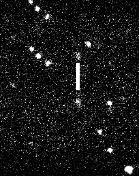
Figure 4.2: K-band image of 3C 54 (at either end of the bar) and surrounding field.

North is at the top, East at the left. The image was composed by mosaicing a series of nine 60-second exposures taken with the waveplate offset at 22.5^∘.)

4.2.2 Second run procedure

For our 1997 run, making use of the instrument’s focal plane mask, we created mosaics of each source by combining seven 60-s exposures at horizontal spacings of $9\hbox{${}^{\prime\prime}$}$ and vertical spacings of $\pm 1\hbox{${}^{\prime\prime}$}$ – see Figure 4.3. This procedure creates rectangular strip images measuring $127\hbox{${}^{\prime\prime}$}\times 20\hbox{${}^{\prime\prime}$}$, of which the central $19\hbox{${}^{\prime\prime}$}\times 16\hbox{${}^{\prime\prime}$}$ displays the maximum sensitivity. The total exposure time, summed over all four waveplate settings, is again listed in Table 4.1.

Figure 4.3: Mosaicing pattern for observing run 2.

4.3 Data Reduction

4.3.1 First run procedure

The raw data from IRCAM3 were stored as Starlink  ndf (foo.sdf) images. These were converted to iraf (foo.imh) format for subsequent analysis by one of two methods: the earliest data to be analysed was handled by conversion to intermediate fits files, which were then read into iraf by its rfits routine; later, when the Starlink  figaro package was enhanced, its new one-step ndf2iraf routine was employed. [Documentation for iraf and Starlink packages can be found at their respective websites, iraf.noao.edu and star-www.rl.ac.uk.]

We reduced the data by marking bad pixels, subtracting dark frames, and flat-fielding. Dr Stephen Eales at Cardiff University (private communication) made available software containing a list of known bad pixels on IRCAM3, which was used to mark the hot and dead pixels; he also provided mosaicing software which ignored such pixels when combining shifted frames to produce a final composite mosaic. The dark frames used were the means of 10-s dark exposures made at the start, middle and end of the night on which the corresponding target images were taken. Flat-fielding frames were obtained by median-combining the nine images of each mosaic without aligning them, and normalizing the resulting image by its mean pixel value. In order to align each set of nine images, we chose a star present on each frame, and measured its position with the apphot.center routine in the iraf package. Using these positions, the nine images were melded into a single mosaic image.

Photometry was performed on the pairs of images of field stars and of radio galaxies in each mosaic using apphot.phot from the iraf package. For each target, we chose one mosaic arbitrarily, and tested this to determine the best photometry aperture as follows: Using the arbitrary mosaic, we performed photometry on the two images of the source at a series of radii increasing in unit pixel steps. The measured magnitude in each aperture decreases as the light included in the aperture increases; we noted the first pair $(r,r+1)$ of radii where the change in magnitude was less than half the measured error on the magnitude. We then earmarked the next radius, $(r+2)$, for use in determining the polarization. In this way, we hope to include most of the source light but as little as possible of the surrounding sky. Where the $(r+2)$ aperture sizes differed for the two channels’ images of the source, we earmarked the larger of the two. This chosen aperture was then used as the photometric aperture on all the mosaics containing the target (i.e. on every waveplate setting from every observing cycle), with iraf output yielding a set of flux counts, magnitudes and errors.

The apphot.phot routine corrects for the sky brightness by measuring the modal light intensity in an annulus around the target; the position of the annulus was chosen in each case such that the outer radius did not extend to the nearest neighbouring object, and the inner radius was normally set one pixel greater than the photometry aperture. (Where we attempted to perform photometry on a knot within a larger structure, the inner radius of the annulus was set sufficiently large to exclude all the knots comprising the object.) The output file of apphot.phot contains data on the sky brightness and consequent errors on each photometric measurement, as well as ‘magnitudes’ (relative to an arbitrary zeropoint) for each target. These values were extracted and analyzed on a PC spreadsheet package (Microsoft Works). The spreadsheet programming follows the scheme described in Chapter 3 and is documented in Appendix B.

The spreadsheet analysis calculated both absolute $(Q,U)$ and normalized $(q,u)$ Stokes parameters for the $\eta_{0}=83\hbox{${}^{\circ}$}$ reference frames, together with the best estimates of the errors in each case. Finally, the optimal normalised Stokes parameters were used as input to fortran routines (also documented in Appendix B) designed to follow Steps 13 thru 18 of Chapter 3’s data reduction scheme. The program’s resultant output values consist of point estimates and confidence intervals of the debiased polarization and orientation measures, and an estimate of the probability that the source is actually polarised.

4.3.2 Second run procedure

Data reduction for the August 1997 run was performed using the standard UKIRT ircamdr software to flat field images, and iraf to align and combine the mosaics. Since spreadsheet analysis of the August 1995 data had shown no source of systematic error, it was not felt necessary to repeat the spreadsheet system of rigorous checks before producing algebraic optimal estimates of the normalised Stokes parameters. Rather, in this case, the images were then averaged to form a single image for each waveplate, as this is equivalent to the algebraic method which gives the best signal-to-noise in the final polarimetry [1998, 1992, 1983]. The 3C 441 data was then combined, at each waveplate position, with our stacked 1995 images. Results are discussed in the next chapter, and summarised in Table 5.1.

4.4 Our Samples

Our first observing run took place on the nights of 1995 August 25, 26, and 27, and covered a sample of seven high-redshift 3C radio galaxies at redshifts $0.7<z<1.2$. These objects were not selected to form any kind of statistically complete sample; rather, they form a representative sample of the different morphologies present in this redshift band. Since this run represented the first known attempt to obtain infrared polarimetry of high redshift radio galaxies, objects known to be bright in the $K$-band were preferred.

The seven objects surveyed included 3C 22 and 3C 41, which are bright and appear pointlike; 3C 114 and 3C 356, which display complex knotted morphologies with large scale alignments between the $K$-band structure and the radio axis; and 3C 54, 3C 65 and 3C 441, which are faint sources with some indication of $K$-band structure. Of these three faint sources, 3C 54 displays an alignment between the $K$-band morphology and the radio axis [1993], 3C 65 shows no preferred direction in its $H$-band structure [1994], and 3C 441 has a broad-band optical polarization which is roughly perpendicular to its radio structure [1992]. Five of the sources (not 3C 22 or 3C 356) were early radio sources observed by Longair [1975].

The second observing run, conducted on the nights of 1997 August 18 and 19, was awarded primarily to study the controversial radio galaxy LBDS 53W091. This galaxy (see §5.2.8) appears to be at least 3.5 Gyr old [1996, 1997] — which is only consistent with its $z=1.552$ redshift in certain cosmologies. The timing of the run also made it possible to re-observe 3C 441, for which our 1995 data were inconclusive, and to observe MRC 0156$-$252, which has the brightest known absolute $V$-band magnitude for a radio galaxy at $z\sim 2$.

Table 4.1 lists all the sources observed together with their redshifts and the rest-frame wavelength of the observed light. As discussed below in §4.6, it is possible to estimate an upper limit on the interstellar polarization imposed on $K$-band light during its passage through our Galaxy. Hence the ned values for the Galactic extinction $A_{B}$ at each observed source and the corresponding upper limits on $p_{\rm K}$ are given in this Table, too.

Table 4.1: Redshifts, integration times, total $B$-band extinctions and upper limits on $K$-band interstellar polarization for our sample of radio galaxies.

Source	IAU form	$z$	$\lambda_{r}$($\mu$m)	$t_{\rm int}$(min)	$l(\hbox{${}^{\circ}$})$	$b(\hbox{${}^{\circ}$})$	$A_{B}$	$p_{K}$
3C 22	0048+509	0.936	1.14	72	122.9	-11.7	1.09	0.76
3C 41	0123+329	0.794	1.23	108	131.4	-29.1	0.17	0.12
3C 54	0152+435	0.827	1.20	135	135.0	-17.6	0.37	0.26
3C 65	0220+397	1.176	0.92	72	141.5	-19.5	0.16	0.11
3C 114	0417+177	0.815	1.21	189	177.3	-22.2	1.26	0.88
3C 356	1723+510	1.079	1.06	99	77.9	34.2	0.10	0.07
3C 441 (1995)	2203+292	0.707	1.29	$\dagger$144	84.9	-20.9	0.34	0.24
3C 441 (1997)	2203+292	0.707	1.29	$\dagger$112	84.9	-20.9	0.34	0.24
LBDS 53W091	1721+501	1.552	0.86	364	76.9	+34.5	0.08	0.06
MRC 0156$-$252	0156$-$252	2.016	0.73	196	208.6	-74.8	0.00	0.00

Key: $z$: redshift; $\lambda_{r}$ (m): rest-frame equivalent of observed-frame 2.2 m; $t_{\rm int}$ (min) : total integration time (min) summed over all waveplate settings ($\dagger$: 3C 441 data from the two runs was pooled giving a composite image of 256 minutes integration time in total) ; $l$ (^∘): Galactic longitude (ned); $b$ (^∘): Galactic latitude (ned); $A_{B}$: Blue-band extinction (mag), from ned, derived from Burstein & Heiles [1982]; $p_{K}$: maximum Galactic interstellar contribution to $K$-band polarization (per cent).

4.5 Calibration

The purpose of the two observing runs made for this project was to obtain polarimetry of faint objects rather than to obtain absolute photometry. Two-channel polarimetry depends on measuring the difference in signal between two channels simultaneously; this eliminates systematic errors which might arise due to imperfect calibration if the channels were instead measured consecutively. Such measurements can be carried out in atmospheric conditions less stringent than those required for accurate photometry. Normalised Stokes parameters, by definition, do not require calibration as they depend on the ratio of two intensities measured by the same system. The source intensities and absolute Stokes Parameters calculated in the course of the data reduction are not reproduced in this thesis; they were expressed in IRCAM3 data number rates throughout the reduction process.

The iraf apphot.phot routine produces a set of output magnitudes for the target objects, relative to a calibrated zero point. We did not use the resultant magnitudes, but the raw data number counts from the photometry aperture, as explained in Appendix B – so it was not necessary to calibrate the zero-point for this purpose. We did not, therefore, observe photometric standard stars as part of the observations for this project.

A polarimetric  standard was measured as part of the August 1997 run to verify the accuracy of the hardware and software forming our polarization reduction chain. The standard star HD 215806, recorded by Whittet et al. [1992] to have polarization 0.55% $\pm$ 0.06% at 77^∘, was measured twice by our data reduction chain. The first measurement yielded 0.36% $\pm$ 0.11% (debiased to 0.35%) at 74^∘ $\pm$ 6^∘: clearly consistent within a $2\sigma$ error box. The second measurement similarly yielded 0.30% $\pm$ 0.11% (debiased to 0.29%) at 73^∘. If instrumental polarization were present, it would increase the measured value, and probably skew it to a different orientation; the agreement between the published and measured orientations confirms that instrumental polarization is negligible in the IRPOL2 chain. The fact that both measurements are lower than the published value is not statistically significant, but is interesting enough that future workers measuring HD 215806 might want to check for variability in its polarization.

In general, it should be noted that polarized standards must be carefully chosen as polarization angle can only be measured to 0.1^∘ and varies with wavelength [1986] — but with such inaccurate measurements being returned for polarization orientations on our radio galaxies, this is hardly relevant in this particular case. Neither would attempting to refine the reference axis zero point $\eta_{0}$ using the standard star add any meaningful accuracy to the measured orientations, given their large error figures.

4.6 Galactic Interstellar Polarization

In the previous chapter, we studied at length the best way to recover a measurement of the true polarization of light from a noisy system. One step remains, however, before the figure obtained can be said to be that of the active galaxy: the interstellar medium of both our own galaxy and the active nucleus’s host galaxy may modify the linear polarization of light passing through it.

Ordinary stars in our own galaxy are not expected to emit intrinsically polarised light; and measured polarization of starlight is presumed to be due to transmission through dust grains. Gehrels [1960] was the first to note that the interstellar polarization varied over visible wavelengths, and subsequent work by Serkowski and colleagues [1974, 1975] found an empirical relationship applicable throughout the visible spectrum:

$$p/p_{\rm max}=\exp[-K\ln^{2}({\lambda}_{\rm{max}}/\lambda)]$$ (4.1)

where ${\lambda}_{\rm{max}}$ is the wavelength at which the polarization peaks, usually around 0.5 m, and empirically in the range 0.3–0.8 m [1975, 1980].

The parameter $K$ was fitted as a constant by Serkowski, Mathewson & Ford [1975], who found the best value to be $K=1.15$. Wilking et al. [1980], however, investigated whether Serkowski’s empirical formula remained valid at infrared wavelengths, and found that a better fit was obtained by taking $K$ to be linearly dependent on ${\lambda}_{\rm{max}}$; an adequate approximation for our purposes is $K=1.7\,$m${}^{-1}\,{\lambda}_{\rm{max}}$. That the empirical formula, so modified, holds up to around 2 m, was confirmed by Martin & Whittet [1990]. The best value of the constant coefficient was refined slightly by Whittet et al. [1992] but the value 1.7 remains an adequate approximation for our purposes.

In general, $p_{\rm max}$ for a given set of galactic co-ordinates is not known. But suppose we take the ratio of polarizations in two wavebands, $V$ and $K$, and rearrange:

$$p_{K}=p_{V}\exp\left\{-3.4{\lambda}_{\rm{max}}\left[\ln\left(\frac{{\lambda}_{\rm{max}}}{\sqrt{\lambda_{K}\lambda_{V}}}\right)\ln\left(\frac{\lambda_{V}}{\lambda_{K}}\right)\right]\right\}.$$ (4.2)

Hence $p_{K}=c.p_{V}$ where $c$ depends on ${\lambda}_{\rm{max}}$ but for $0.3<{\lambda}_{\rm{max}}<0.8$ we find $0.15<c<0.30$.

An empirical upper limit for $p_{V}$ (expressed as a percentage) is given by Schmidt–Kaler [1958] as $p_{V}\leq 9E_{B-V}$ and typically, $p_{V}=4.5E_{B-V}$. [Clarke & Stewart [1986, §4.2] point out that determinations of an empirical upper limiting polarization also tend to find an empirical lower limit, suggesting imperfect debiasing, and that the true empirical upper limit is in fact lower than the one determined.] It is well established [1979, 1983, 1985] that the ratio of total to selective extinction is $A_{V}/E_{B-V}\sim 3$; and so we can use the extinctions $A_{B}$ [1982, figures can be obtained from the ned database] to obtain $E_{B-V}=A_{B}-A_{V}=A_{B}/4$.

Taking the maximum values, $c=0.3$ and $p_{V}\leq 9E_{B-V}$, we find an upper limit for infrared polarization $p_{K}\leq 0.7A_{B}$. We have seen (Table 4.1) that none of the objects surveyed for this thesis lie beyond regions of our Galaxy with $A_{B}>1.3$, and all but two have $A_{B}<0.4$, so the Galactic medium cannot contribute more than 1.2% to the $K$-band polarization of the two high-extinction sources, or more than 0.3% to $K$-band polarization of any of the others. A further check can be made by measuring the polarizations of sources (presumably intrinsically unpolarized stars) which lie in the same fields as our target objects (this will be commented on during discussions of individual targets in the next chapter).

Like our own Galaxy, the host galaxies of the active nuclei may contain dust regions capable of polarizing light passing through them. Goodrich & Cohen [1992] argue that 3C 109 is polarised in this way; 3C 234 could be a similar example [1998]. Such polarization effects affect the observed $K$-band light at its rest-frame wavelength and will be considered in the context of the discussion of individual sources – since the source of such polarization is, by definition, the host galaxy of an active galactic nucleus. The possibility of polarizing effects being produced at intermediate wavelengths by any intergalactic medium cannot be ruled out a priori, but we invoke Occam’s Razor to assume the absence of significant amounts of any intergalactic medium without evidence to the contrary (e.g. from the observed colours of the target galaxies).

Chapter 5 General Observations and Individual Objects

Look up at the heavens and count the stars – if indeed you can count them.
— Genesis 15:5 (NIV).

The observational datasets obtained were reduced and analysed using the procedure described in the previous chapter. As is recommended for polarimetry, the normalised Stokes parameters $q$ and $u$ were obtained; the reference axis for IRPOL2 is $\eta_{0}=83\hbox{${}^{\circ}$}$, i.e. that $q>0,u=0$ corresponds to a polarization orientation of 83^∘ E of N and that for $q=0,u>0$, the polarization orientation is 128^∘. Table 5.1 gives the polarizations of all target objects and associated objects, but not of the field objects also analyzed.

Some target objects displayed extended structure: Reference is made in the text of this chapter to the ‘moment analysis’ of Dunlop & Peacock [1993], who devised an automated routine to evaluate a position angle for the extended structure they saw in $K$-band sources. For those sources in which there are clear distinct components to the structure, the identification of these components is given on the labelled images which follow. In most of our images, the target object is labelled T; other objects have been labelled following earlier maps in the literature, where available. Composite images are shown in each case with the images from all waveplate positions stacked together; in some cases, edited images are also provided where one set of images from the Wollaston prism’s ‘double image’ have been removed using the image patching facilities of the starlink gaia package.

Table 5.1: Observational results of $K$-band polarimetry of our nine target radio galaxies and associated objects.

Source	$r$(′′)	$q(\sigma_{q})$(%)	$u(\sigma_{u})$(%)	$P\pm\sigma_{P}$(%)	$2\sigma$.UL	Prob	$\theta$(∘)	$\sigma_{\theta}$(∘)
3C 22	2.6	-1.3 (1.4)	-3.2 (1.4)	3.3 $\pm$ 1.4	-	0.95	27	-71	+17
3C 41	2.3	+0.8 (1.1)	-3.1 (1.1)	3.1 $\pm$ 1.1	-	0.98	45	-14	+79
3C 54	4.0	-1.4 (2.5)	-6.0 (2.5)	5.9 $\pm$ 2.6	-	0.94	32	-79	+17
3C 65	2.9	-4.3 (4.2)	-1.2 (4.0)	2.2 $\pm$ L4.5	10	0.42	1	$\pm$71
3C 114 (Whole)	3.6	+11 (3)	-4.1 (2.7)	11 $\pm$ 3	-	0.99	73	-21	+34
3C 114 (Knee)	1.7	+3.0 (1.6)	+4.3 (1.8)	5 $\pm$ 1.7	-	0.99	111	-63	+14
3C 356 (Whole)	4.0	-10 (5)	+3.5 (6)	9 $\pm$ 5	16	0.85	172	$\pm$22
3C 356 $a$ (North)	2.3	-13 (8)	+4.6 (8)	13 $\pm$ 8	41	0.62	164	$\pm$25
3C 356 $b$ (SE)	2.6	-10 (9)	-19 (17)	19 $\pm$ 15	24	0.78	24	-54	+33
3C 441 a	3.1	+4 (5)	-0.7 (5)	1 $\pm$ L6	10	0.46	78	$\pm$51
3C 441 B$\ddagger$	3.1	+0.5 (5)	-1.7 (5)	0.1 $\pm$ L2.8	7	0.14	47	$\pm$59
3C 441 c$\ddagger$	3.1	+1.3 (12)	+10 (11)	3.5 $\pm$ L16	24	0.54	124	$\pm$45
3C 441 E	2.6	+5 (12)	+19 (13)	18 ${}^{+9}_{-8}$	36	0.91	120	$\pm$15
3C 441 F	2.0	+6 (19)	+16 (22)	6 $\pm$ L28	43	0.48	118	$\pm$48
3C 441 G	2.6	-0.1 (13)	-6 (13)	0.3 $\pm$ L10	21	0.18	38	$\pm$59
3C 441 H	2.3	-12 (14)	-9 (15)	7 $\pm$ L22	33	0.67	11	$\pm$38
LBDS 53W091 $\natural$	1.1	0 (17)	-7.5 (22)	0.4 $\pm$ L8	31	0.11	38	$\pm$60
LBDS 53W091 $\flat$	1.1	+0.6 (16)	-3.4 (18)	0.17 L,U	22	0.20	43	$\pm$60
Object 3a $\natural$	1.1	-12 (18)	+17 (18)	16 $\pm$ L14	43	0.70	146	$\pm$24
Object 3a $\flat$	1.1	-4.5 (21)	+21 (20)	10 $\pm$ L21	46	0.67	134	$\pm$36
MRC 0156$-$252	2.3	-2.5 (7)	+1 (7)	0.14 $\pm$ L4.3	10.5	0.14	161	$\pm$59
MRC 0156$-$252	2.7	-0.5 (8)	-0.5 (8)	0.04 L,U	4	0.01	60	$\pm$60
MRC 0156$-$252	3.4	+0.4 (8)	+0.8 (9)	0.05 L,U	5.5	0.01	114	$\pm$60

Key: Source: Source name and component ($\natural$: natural image; $\flat$: ‘despiked’ image; $\ddagger$: data is based on 1995 observations only); r: radius of photometry aperture (arcseconds); $q\pm\sigma_{q},u\pm\sigma_{u}$: normalized Stokes Parameters (per cent) with respect to 83^∘ E of N; $P\pm\sigma_{P}$: percentage polarization (debiased) with 1$\sigma$ error (^L — the $1\sigma$ lower limit for polarization is zero; ^L,U — the $1\sigma$ ‘confidence interval’ is identically zero even though the best point estimate polarization is non-zero); Prob: the probability that there is underlying polarization, given by Equation 3.32; $2\sigma$.UL: $2\sigma$ upper limit (in per cent) for polarization in objects unlikely to be polarised; $\theta\pm\sigma_{\theta}$: Electric vector orientation E of N (^∘).

5.1 Have We Detected Polarization?

Equation 3.32 allows us to quantify the probability that a given object is polarised. The probabilities of each object being polarised are listed in Table 5.1. Three of our nine sources have a 95% or better probability of being polarised; and of these, 3C 22 and 3C 41 are polarised at the 3 per cent level, and 3C 114 at the 12 per cent level.

The number of prominent starlike objects (in addition to the target) featuring on the 1995 set of 3C object mosaics varies between one and seven, depending on the target. (We will refer to these as ‘stars’ but have no spectroscopic evidence to confirm their identity as such.) Where possible, we have performed polarimetry on these stars; out of the 21 stars so observed, only one has a greater than 95% probability of being polarised. This object was a bright starlike object on the mosaic containing 3C 114, but is only polarised at the 0.7 per cent level, which is explicable by the interstellar medium (see Table 4.1). Even without such special pleading, it would not be surprising for random noise to cause one star out of 21 to appear to be polarised at such a level.

Within the bin of sources having a probability 80-95% of being polarized, fall three further stars; of these, one is extremely faint, and another appears to be polarised at only the 0.3 per cent level. The third falls on the same mosaic as 3C 54, and appears to be polarised at the 5.6 $\pm$ 2.6 per cent level, with a 94% chance of the polarization being genuine. This star, however, straddles the edge of three of the nine component frames of the mosaics, so the validity of the result is called into question. Two of our sources also fall in the 80-95% probability bin: 3C 54 itself, polarised at the 6 per cent level, and 3C 356, at the 9 per cent level. (Object E of the 3C 441 complex may also fall in this bin, on the basis of the pooled 1995 and 1997 observations.)

For the 1995 observations, given that 17 out of 21 stars, but only 2 out of 7 sources, have a probability of less than 80% of being polarised at all, we feel confident of having detected polarization in three 3C sources, and possibly in a further two. The three targets for the 1997 run were faint objects in comparison to most of those observed in the earlier run: one component of the 3C 441 complex displays marginal evidence for polarization, but there is no strong evidence for polarization in 53W091 or MRC 0156$-$252.

5.2 Individual Objects

In the following object-by-object discussion, we will examine each target object in the context of other observational data about the same object from the literature. Evidence for parallel or perpendicular alignments will be noted, but discussion of the implications of our data for the properties of the central engines and host galaxies will be deferred to the next chapter. In this context, the Hubble Space Telescope  is abbreviated HST.  Certain papers will be cited very frequently, and will be abbreviated in this chapter: Dunlop & Peacock [1993] will be denoted D&P, Leyshon & Eales [1998] is abbreviated L&E, and a series of papers by Best, Longair & Röttgering will be denoted BLR-I [1996], BLR-II [1997], and BLR-III [1998].

The polarizations of other objects on the target frames will be noted here, using normalised Stokes parameters of the form $\tilde{q}\pm\sigma_{\tilde{q}},\tilde{u}\pm\sigma_{\tilde{u}}$, as obtained through Data Reduction Step 9; estimates of $P$ (debiased) and orientation will also be quoted. Since the probability that these objects are polarized is low, formal errors on the nominal degree and angle of polarization are not quoted; these can easily be calculated from the normalised Stokes parameters and their errors if required. These field objects serve as useful controls which would immediately indicate regions of high $K$-band Galactic polarization – though they cannot, by themselves, rule out the presence of polarizing material beyond their locations.

5.2.1 3C 22

Structure

Radio galaxy 3C 22 appears close to three other starlike objects which we have designated A, B and C (see Figure 5.1); our star A is object C in the notation of Riley, Longair & Gunn [1980]. UKIRT $K$-band imaging shows a red companion about 4^′′ to the south-west. This is placed at bearing 237^∘ from the core by D&P’s moment analysis algorithm; they note that it was not apparent in the optical image of McCarthy [1988]. Our $K$-band image shows no evidence for extended structure, though this companion is clearly visible in the UKIRT $K$-band image of BLR-II, and also (clearly resolved as a separate object) in their HST  image. At the resolution of the HST, the true bearing of this companion is seen to be 208^∘ $\pm$ 1^∘.

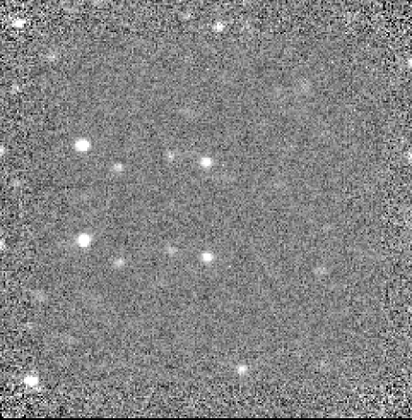
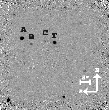
Figure 5.1: Images of 3C 22.

Raw (above) and annotated negative (below) $K$-band structure of 3C 22 – lower channel objects have been edited out of the negative image.

The most recent review of the radio, visible and infrared properties of 3C 22 (BLR-II §3, and references therein) finds two slight extensions in HST  images of 3C 22 itself. They find that the nucleus can be fitted as a combination of a point source and a de Vaucouleurs law, with the point source contributing 37% of the total $K$-band intensity (BLR-III). The $J-K$ colour of 3C 22 is typical of a radio galaxy at its redshift, but the $R-K$ colour is one of the reddest of the 3CR subsample of D&P. The $\sim 0.5\hbox{${}^{\prime\prime}$}$ extensions are interpreted (BLR-II) as a possible close companion, marginally redder than the core, due south (bearing $\sim 180\hbox{${}^{\circ}$}$), and as a blue extension slightly south of west (bearing $\sim 250\hbox{${}^{\circ}$}$).

The radio position angle of 3C 22 is given as 102^∘ (equivalently 282^∘) by Schilizzi, Kapahi & Neff [1982] and Jenkins, Pooley & Riley [1977]; the 8.4 GHz VLA radio map of BLR-II confirms this to $\pm 1\hbox{${}^{\circ}$}$.

Polarimetry

Polarimetry results for 3C 22, designated T (for Target), and the three field objects, are reported in Table 5.2. All three companions produce normalised Stokes parameters around $1\sigma$. 3C 22 itself has a 95 per cent chance of truly being polarised, and its debiased polarization is $3.3\pm 1.4$%. We expect that no more than 0.8% is due to the interstellar medium; most of the polarization is therefore intrinsic to the source. In the optimal 2.6^′′ radius aperture, the two extended features observed by the HST  will be included, but light from the red SW companion at 4^′′ will not.

Table 5.2: Normalised Stokes Parameters: Objects in 3C 22 field.

Source	$q$	$\sigma_{q}$	$u$	$\sigma_{u}$	Prob	$P$(%)	$\theta(\hbox{${}^{\circ}$})$
A	-3.05	3.92	-3.84	4.03	53.2	4.22	18.8
B	-3.13	2.23	2.62	2.23	81.3	3.77	153.0
C	-0.61	0.60	-0.72	0.58	72.0	0.84	17.9
T	-1.27	1.38	-3.16	1.38	95.3	3.26	27.0

Key: Source objects are as identified in Figure 5.1, T is 3C 22; $q$ and $u$ are ‘best estimator’ normalised Stokes parameters (%) with R-axis at $\eta_{0}$=83^∘. Prob (%) is the probability of a nonzero polarization being present; $P$(%) and $\theta(\hbox{${}^{\circ}$})$ are the nominal debiased degree of polarization and its orientation.

The measured orientation of the $E$-vector is ${+27}^{+17}_{-71}\hbox{${}^{\circ}$}$ East of North. The error is large, but at a nominal 27^∘ $(=207\hbox{${}^{\circ}$})$ our measurement suggests that the true direction is more likely to be perpendicular to the radio axis, than parallel to it. Comparing the polarization orientation with extended structure, we find that the blue western optical extension is not remarkably close to being perpendicular or parallel to the polarization orientation; the red southern extension/companion might be in parallel alignment for a plausible error in the orientation angle. The red companion to the SW at bearing 208^∘ effectively lies on the nominal polarization axis.

Jannuzi [private communication] [1999] has performed imaging polarimetry on 3C22 at shorter optical wavelengths, and reports $3\sigma$ upper limits in $V$ and $H$ of 5 per cent and 3 per cent respectively.

5.2.2 3C 41

Structure

3C 41 appears with a field object labelled B (see Figure 5.2) following the notation of Riley, Longair & Gunn [1980]. The radio position angle of 3C 41 is 147^∘ [1975], confirmed to $\pm 2\hbox{${}^{\circ}$}$ by the 8.4 GHz VLA radio map of BLR-II.

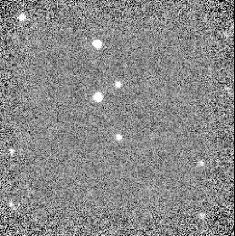
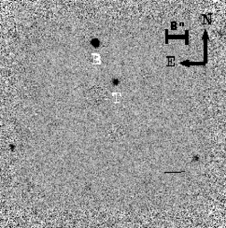
Figure 5.2: Images of 3C 41.

Raw (above) and annotated negative (below) images of 3C 41 – lower channel objects have been edited out of the negative image.

Our $K$-band image shows no evidence for extended structure, but BLR-II detect two distinct companions in their HST  image which can also be discerned as ‘extensions’ in their UKIRT $K$-band image; the WSW extension can also be distinguished in the $K$-band contour map of Eisenhardt & Chokshi [1990], who note that $K$-band emission from the source extends for at least 12^′′. Both companions are more than a magnitude bluer than the core: positioned ESE and WSW of the core they lie on a line oriented at a position angle of $127\hbox{${}^{\circ}$}\pm 2\hbox{${}^{\circ}$}$. They are hence misaligned with the radio axis by about 20^∘ (BLR-II).

Polarimetry

Normalised Stokes parameter measurements for 3C 41 (Target T) and field object B are given in Table 5.3. 3C 41 has a 98 per cent chance of having a nonzero underlying polarization, which we measure to be 3.1 $\pm$ 1.1 per cent. Our upper limit for extinction-induced polarization is only 0.1 per cent, so we are confident of having detected intrinsic polarization in this object. The orientation of the $E$-vector is ${+45}^{+79}_{-14}\hbox{${}^{\circ}$}$ East of North.

Table 5.3: Normalised Stokes Parameters: Objects in 3C 41 field.

Source	$q$	$\sigma_{q}$	$u$	$\sigma_{u}$	Prob	$P$(%)	$\theta(\hbox{${}^{\circ}$})$
B	-0.27	0.16	0.18	0.16	86.7	0.30	156.6
T	0.82	1.11	-3.08	1.11	98.4	3.08	45.4

Key: Source objects are as identified in Figure 5.2, T is 3C 41; $q$ and $u$ are ‘best estimator’ normalised Stokes parameters (%) with R-axis at $\eta_{0}$=83^∘. Prob (%) is the probability of a nonzero polarization being present; $P$(%) and $\theta(\hbox{${}^{\circ}$})$ are the nominal debiased degree of polarization and its orientation.

Jannuzi [private communication] [1999] have firm $V$ and $H$ band polarizations for this source: at $V$, the polarization is 9.3 $\pm$ 2.3% at 58^∘$\pm$ 7^∘; at $H$, the polarization is 6.6 $\pm$ 1.6% at 57^∘$\pm$ 7^∘. The $E$-vector orientations in the three wavebands are consistent with one another. We therefore find a very good perpendicular alignment between the radio structure and optical polarization axes; the small errors on the $V$ and $H$ polarizations show that their alignment is perpendicular to the radio structure rather than the HST  visible structure. Our $K$-band polarization orientation error is large enough to permit it to be perpendicular to the optical structure rather than the radio; but Occam’s razor invites us to assume that the true orientation in $K$ should correspond to that in $V$ and $H.$

5.2.3 3C 54

Structure

No wide-aperture image of 3C 54 and its surrounding field could be found in the literature; the target was identified on the grounds that it lay close to the nominal position at the centre of our UKIRT images and displayed a slight southern extension corresponding to that seen in D&P’s $K$-band contour map. This extension is known to be more prominent in $K$ than in $J$ [1990], and is also known as structure $b$ at a bearing of 200^∘ in the $R$-band [1987a]. Bright field objects have been designated A to D as indicated in Figure 5.3; the target object itself may be seen more clearly in Figure 4.2.

The position angle of 3C 54’s radio structure is 24^∘ [1975]. A moment analysis gives the $K$-band structure’s major axis orientation as 27^∘ (D&P), essentially parallel to the radio axis; the visible continuum structure is reported as very similar to the infrared, while the [O ii] emission is less similar, although elongated in the same sense [1987a, 1988]. The $J-K$ colour is typical of similar objects at the same redshift [1990].

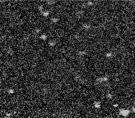
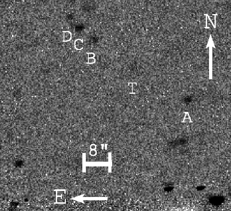
Figure 5.3: Images of 3C 54.

Raw (above) and annotated negative (below) images of 3C 54 – lower channel objects have been edited out of the negative image.

Polarimetry

The target and those field objects (A, B) bright enough to be analysed have their normalised Stokes parameters reported in Table 5.4. The probability that 3C 54 is polarised is 94 per cent; our measured value of polarization is 5.9 $\pm$ 2.6% at ${+32}^{+17}_{-79}\hbox{${}^{\circ}$}$ East of North. Dust is not expected to contribute more than 0.3%. We therefore appear to have a genuine polarization oriented parallel to both the radio and extended optical structures of this source.

Table 5.4: Normalised Stokes Parameters: Objects in 3C 54 field.

Source	$q$	$\sigma_{q}$	$u$	$\sigma_{u}$	Prob	$P$(%)	$\theta(\hbox{${}^{\circ}$})$
A	1.82	2.75	2.41	3.17	39.3	1.08	109.5
B	5.82	2.50	-0.35	2.66	93.4	5.54	81.3
T	-1.36	2.52	-6.01	2.55	94.6	5.88	31.6

Key: Source objects are as identified in Figure 5.3, T is 3C 54; $q$ and $u$ are ‘best estimator’ normalised Stokes parameters (%) with R-axis at $\eta_{0}$=83^∘. Prob (%) is the probability of a nonzero polarization being present; $P$(%) and $\theta(\hbox{${}^{\circ}$})$ are the nominal debiased degree of polarization and its orientation.

5.2.4 3C 65

Structure

Source 3C 65 was identified using the chart provided by Gunn et al. [1981], and its field objects have been designated A–G as indicated in Figure 5.4.

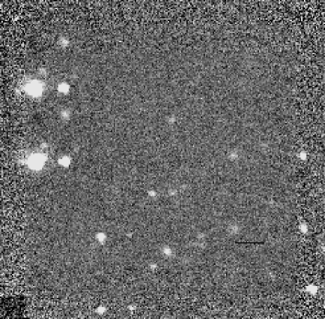
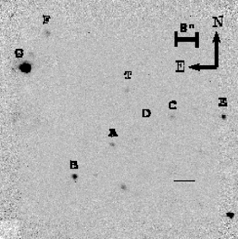
Figure 5.4: Images of 3C 65.

Raw (above) and annotated negative (below) images of 3C 65 – lower channel objects have been edited out of the negative image.

BLR-I describe 3C 65 as a fairly round central object, and one of the reddest in the 3CR sample with $V-K\sim 6$. A 4000 Å break in the off-nuclear spectrum [1995, 1995] indicates the presence of an old stellar population, $\sim 3-4$ Gyr. Their HST  visible image shows that 3C 65 is slightly elongated NE–SW. Both their HST  and UKIRT images show a blue companion galaxy 3^′′ to the west, lying approximately on the radio axis, but this was too faint to be distinguished from the noise on our $K$-band images. Their 8.4 GHz VLA radio map shows a radio structure at position angle $100\hbox{${}^{\circ}$}\pm 3\hbox{${}^{\circ}$}$.

Lacy et al. [1995] have claimed evidence for an infrared point source, possibly an obscured quasar nucleus, in the infrared core of 3C 65; Rigler & Lilly [1994], however, found that the infrared profile could be satisfactorily fitted by a de Vaucouleurs law. BLR-II & III’s HST  image of 3C 65 also yields an adequate fit for a cD galaxy (de Vaucouleurs law plus faint halo) model.

Polarimetry

Field object D proved too faint for accurate photometry; normalized Stokes parameters for 3C 65 (target T) and the other field objects are reported in Table 5.5. Our polarimetry indicates a 57% probability that 3C 65 is an unpolarized  source; our nominal polarization orientation angle (from Table 5.1) is perpendicular to the radio axis, but the statistical significance of our $K$-band polarization measurement is at best dubious.

Table 5.5: Normalised Stokes Parameters: Objects in 3C 65 field.

Source	$q$	$\sigma_{q}$	$u$	$\sigma_{u}$	Prob	$P$(%)	$\theta(\hbox{${}^{\circ}$})$
A	-0.99	4.00	-1.51	6.58	4.6	0.09	21.3
B	4.21	15.12	1.97	14.73	4.6	0.23	95.5
C	2.12	4.32	2.95	4.20	30.6	1.27	110.2
E	-0.07	2.29	2.41	2.21	44.9	1.87	128.8
F	-0.71	5.16	-2.81	3.07	33.0	1.00	30.9
G	-0.05	0.41	0.14	0.44	5.4	0.01	137.2
T	-4.33	4.25	-1.17	4.03	42.9	2.12	0.6

Key: Source objects are as identified in Figure 5.4, T is 3C 65; $q$ and $u$ are ‘best estimator’ normalised Stokes parameters (%) with R-axis at $\eta_{0}$=83^∘. Prob (%) is the probability of a nonzero polarization being present; $P$(%) and $\theta(\hbox{${}^{\circ}$})$ are the nominal debiased degree of polarization and its orientation.

5.2.5 3C 114

Structure

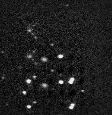
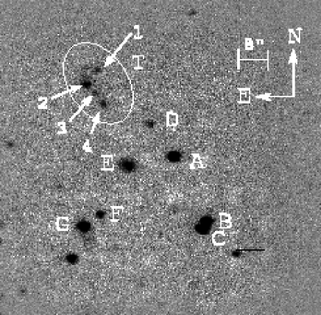
Figure 5.5: Images of 3C 114.

Raw (above) and annotated negative (below) images of 3C 114 – lower channel objects have been edited out of the negative image.

The field containing 3C 114 is illustrated in Figure 5.5; a close-up image detailing the structure of knots is shown as Figure 5.6. Its distinctive shape (D&P) makes it easily identifiable; it consists of at least four knots, where the brightest knot forms the knee of a $\Gamma$-shaped structure. The radio position angle of 3C 114 is 44^∘ [1990], and the large size of the radio structure (54^′′) is noteworthy.

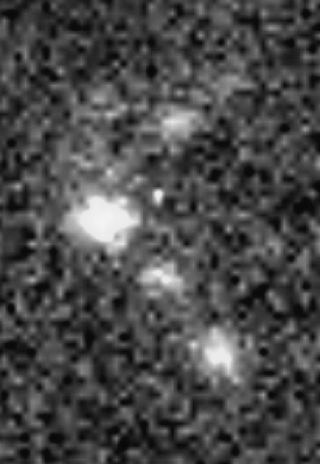
Figure 5.6: Close-up of the $K$-band structure of 3C 114.

(North is at the top, East is on the left.)

D&P’s $K$-band contour map reveals more detail in the structure of 3C 114 with additional knots of lower intensity close to the four obvious ones in our image; the three major knots forming the NE–SW line seem to be joined by an underlying luminous structure. This structure dominates a moment analysis of the whole source, yielding a $K$-band optical structure angle of 52^∘, close to the 44^∘ for radio structure.

Polarimetry

Only the knee knot proved bright enough to analyze on its own; Table 5.1 includes results for both that knot and the structure as whole. There is a probability in excess of 99 per cent that there is genuine polarization in both the knee knot and the overall structure.

Table 5.6: Normalised Stokes Parameters: Objects in 3C 114 field.

Source	$q$	$\sigma_{q}$	$u$	$\sigma_{u}$	Prob	$P$(%)	$\theta(\hbox{${}^{\circ}$})$
A	0.77	0.23	0.12	0.29	99.7	0.77	87.3
B	5.56	3.20	0.78	3.21	78.5	5.14	87.0
C	5.55	3.20	0.67	3.21	78.3	5.12	86.5
D	0.12	2.86	0.43	2.85	1.2	${\ddagger}$	${\ddagger}$
E	-0.80	1.12	-1.39	1.13	63.4	1.41	23.1
F	1.90	2.81	3.29	2.74	61.2	3.32	113.0
G	5.28	3.31	-0.18	3.14	72.0	4.75	82.0
T0	11.19	3.07	-4.14	2.68	100.0	11.73	72.9
T2	3.00	1.63	4.31	1.77	99.0	5.10	110.6

Key: Source objects are as identified in Figure 5.6, T0 is the whole of 3C 114 and T2 its ‘knee’ knot; $q$ and $u$ are ‘best estimator’ normalised Stokes parameters (%) with R-axis at $\eta_{0}$=83^∘. Prob (%) is the probability of a nonzero polarization being present; $P$(%) and $\theta(\hbox{${}^{\circ}$})$ are the nominal debiased degree of polarization and its orientation. ${\ddagger}$: These data are not given for object D; it seems unpolarized and our debiasing algorithm did not converge to a solution.

We measured polarization in the knee of 5.1 $\pm$ 1.7 per cent, at ${+111}^{+14}_{-63}\hbox{${}^{\circ}$}$ East of North. Overall, the whole object has a polarization of 11.7 $\pm$ 3.0 per cent at ${+73}^{+34}_{-20}\hbox{${}^{\circ}$}$. The extinction contribution could be as high as 0.9 per cent, but our detections of polarization are much higher than this, so the polarization appears to be intrinsic. With the radio and optical structure axes at $\sim 48\hbox{${}^{\circ}$}$, there is no clear alignment of polarization either parallel or perpendicular to the structure.

5.2.6 3C 356

Structure

Source 3C 356 has provoked much discussion in the literature. The radio structure is a large (72^′′) double with position angle 161^∘ [1989]. D&P’s $K$-band contour map displays three knots: two brighter knots lying NW–SE along the radio axis, and a much fainter knot off-axis to the south-west. Both bright knots are associated with radio cores [1993], and it is not clear which hosts the radio source; both lie at $z=1.079$ (BLR-II). In the convention established by LeFèvre, Hammer & Jones [1988b], and used by others [1990, 1990, 1994, 1997], the NW component is denoted $a$ and the SE component, $b$. Fainter components are labelled following BLR-II.

The SE component, $b$, is elongated roughly perpendicularly to the radio source [1992]. Lacy & Rawlings [1994] note how this SE radio core has a flatter spectral index and may be the host to the radio source, with galaxy $a$ interacting with the jet; $b$’s spectral index is $\alpha\approx 0.1$ between 8.4 GHz and 5 GHz (BLR-II), which is typical of a compact core in an extended radio source. Eales & Rawlings [1990] also favoured $b$ as the radio core due to its colour, magnitude and shape being typical of radio galaxies.

The more recent HST  observations of BLR-I & II, however, reveal the NW component $(a)$ to have the same dumbbell morphology they observe in other radio galaxy hosts, while the SE object $(b)$ seems much more diffuse than their other 3CR sources. Component $a$ is also favoured as the radio core by Eisenhardt & Chokshi [1990] and McCarthy [1988]: it has bluer infrared–optical colours and dominates the visible continuum and [O ii] images. D&P dispute LeFèvre et al.’s [1988a] claim that $b$ has the bluer colours; HST  observations show that $b$ is redder, but some of the diffuse emission is as blue as $a$ [1990, BLR-II]. Component $a$’s spectral index is that of a compact steep spectrum source, $\alpha\approx 1.1$, and the 8.4 GHz radio flux is only a quarter of that of component $b$ (BLR-II).

BLR-III find that 3C 356 (presumably meaning the NW component, measured in a 5^′′ aperture), can be well modelled purely by a de Vaucouleurs profile. A 4000 Å spectral break has been detected in both $a$ and $b$ [1994], indicating that both components contain stars and are aged at least 10 Myr. D&P’s $K$-band image moment analysis algorithm gives a position angle of 159^∘ for the overall structure, but Cimatti et al. [1997] state that the two $K$-band knots taken together as a single structure lie at a position angle of 145^∘, with the two dumbbell components of $a$ separated along a line at 152^∘.

Our $K$-band image of 3C 356 (Figure 5.7) reveals the three knots indicated: $b$ at the south-east, $a$ at the north-west, and the very faint south-west component denoted $d$ in the HST  image of BLR-II. A prominent field star, object C of Riley, Longair & Gunn [1980], is also labelled.

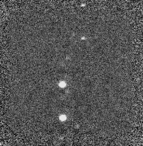
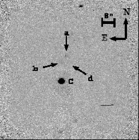
Figure 5.7: Images of 3C 356.

Raw (above) and annotated negative (below) images of 3C 356 – lower channel objects have been edited out of the negative image.

Polarimetry

Cimatti et al. [1997] have obtained Keck I spectropolarimetry of 3C 356’s two main components for light emitted between 200 nm and 420 nm. They find polarization which rises towards the ultraviolet: source $b$’s polarization was low, reaching $4.0\pm 1.2\%$ at 200 nm, while $a$’s polarization rose from 3% at 420 nm to about 15% at 200 nm. A distinct Mg ii $\lambda$2800 line was also detected in component $a$’s light, polarized to the same degree as the continuum, and with the same orientation of 64^∘.

The perpendicular axis to the polarization vector lies at 154^∘, and is therefore within two degrees of the dumbbell separation observed in object $a$, nine degrees anticlockwise of the radio structure, and seven degrees clockwise of the $a$-$b$ axis.

Our $K$-band images show the galaxy in light emitted in a band centred on 1060 nm. The SW knot (object $d$) was not bright enough to permit polarimetry. Normalised Stokes parameters for the two major components ($a$, $b$), the 3C 356 complex as a whole (T0) and field object C are recorded in Table 5.7. We find no strong evidence for $K$-band polarization in 3C 356; the probability of non-zero $K$-band polarization being present in $a$ and $b$ is 62% and 79% respectively, and the polarization orientations derived from our noisy measurements do not include 64^∘ in their $\pm 1\sigma$ error boxes.

Table 5.7: Normalised Stokes Parameters: Objects in 3C 356 field.

Source	$q$	$\sigma_{q}$	$u$	$\sigma_{u}$	Prob	$P$(%)	$\theta(\hbox{${}^{\circ}$})$
C	0.15	0.15	0.27	0.21	71.0	0.27	113.4
T0	-9.64	4.94	0.35	5.63	85.1	8.97	172.0
$a$	-13.32	7.95	4.60	8.38	62.4	18.76	23.9
$b$	-10.10	9.39	-18.88	16.62	78.9	12.90	163.5

Key: Source objects are as identified in Figure 5.7, T0 is the whole structure of 3C 356; $q$ and $u$ are ‘best estimator’ normalised Stokes parameters (%) with R-axis at $\eta_{0}$=83^∘. Prob (%) is the probability of a nonzero polarization being present; $P$(%) and $\theta(\hbox{${}^{\circ}$})$ are the nominal debiased degree of polarization and its orientation.

5.2.7 3C 441

Structure

3C 441 appears in a rich field (Figure 5.8) with five neighbours; identification of the radio core is based on the observations of Riley, Longair & Gunn [1980] and is apparently confirmed by the work of McCarthy [1988] and of Eisenhardt & Chokshi [1990]. Figure 5.8 is based on our August 1995 data (L&E) which was taken without a focal plane mask. The objects labelled a and c, and the position of unseen object d, follow the notation of Lacy et al. [1998]; the star B is labelled as in Riley et al. [1980], and the remaining objects are labelled E thru H. An unedited image with scale bar is given later as Figure 5.9. Object a itself is shown to have 0.5 mag bluer extension protruding to the south-west in its HST  image (BLR-II). Object c is more compact in the infrared than in $R$-band imaging, while object a appears more extended east-west in the infrared than in $R$ [1990, BLR-II].

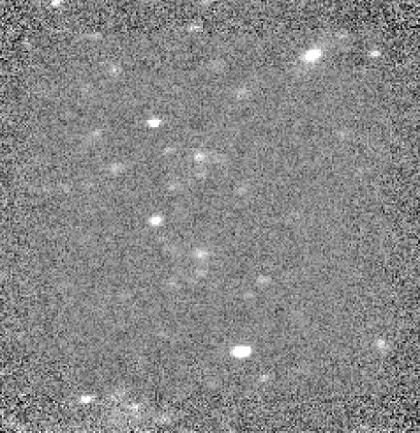
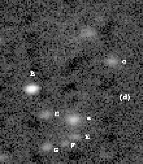
Figure 5.8: Images of 3C 441.

Raw (above) and annotated negative (below) images of 3C 441 – lower channel objects have been edited out of the negative image. North is at the top and East to the left; the scalebar is given in Figure 5.9.

Fabry-Perot imaging by Neeser [1996] shows that none of the other objects in the field lie within a velocity range $(-1460,+1180)$ km s^-1 of 3C 441 itself, but since the $J-K$ colours of most of these neighbouring objects lie between 1.6 and 1.85 (BLR-II), 3C 441 could be part of a cluster. Neeser [1996] questions whether the identification of 3C 441 is correct – arguing that it may in fact be our object F. Recent imaging by Lacy et al. [1998] suggests that 3C 441’s jet is impacting object c to its north-west – this object has the same infrared colour as object a and is the only other area of strong [O ii] emission in the field [1990, BLR-II].

The 5 GHz radio map of 3C 441 [1975] shows a double radio source with the separation between sources running East-West, and extended structure trailing off to the South-East. Lacy et al. [1998] show that the North-West jet (at 8 GHz) is deflected to the south where it would otherwise have encompassed object c.

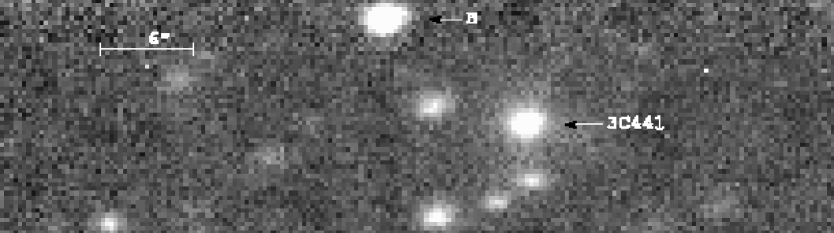
Figure 5.9: 3C 441: stacked $K$-band image of August 1995 and August 1997 data.

Total integration time 4 hours 16 minutes. [1 hour 52 minutes (1997) plus 2 hours 24 minutes (1995).] North is at the top, East at the left. The star B is labelled as in Riley, Longair & Gunn [1980].

nb Any future worker planning to observe 3C441 should note that there is a $z=4.4$ quasar which falls in the same field [1988]. Judicious planning could enable studies of this object to be conducted in parallel with the radio galaxy.

Polarimetry

It is known that 3C 441 has a broad-band optical polarization of 1.5 $\pm$ 0.7% at 70^∘ $\pm$ 13^∘ in a 2^′′ diameter aperture about the core: this orientation is roughly perpendicular to the radio structure [1992]. Our 1995 and 1997 images were stacked together to obtain polarization measurements of objects a (the putative core of 3C 441) and E thru H; the 1995 data alone was used to obtain polarization data on B and c. Given the uncertainty posited by Neeser [1996] over the identification of 3C 441, and the interest in object c of Lacy et al. [1998], we performed polarimetry on all the objects on the field, with the full results presented in Table 5.1.

The only object with a strong indication (90 per cent chance genuine) of polarization is E. The orientation is 120^∘, which would be roughly parallel with the radio jet — but the position angle which E makes with the presumed core a is close to 0^∘, which means that a model of E scattering light from a is possible. It would not be necessary for light from a to be beamed into E; if E subtends only a small solid angle of the light emitted by a, any light from a scattered by E would be quasi-unidirectional.

There is a weak indication that object c might be polarised. If so, the best estimate is 3.5% polarization at 124^∘ – an orientation roughly parallel to any jet from a which might be scattered into our line of sight. Similarly, object H might possibly be polarised at 6.7%, 11^∘, which is roughly perpendicular to its line of sight with a, and parallel to that with B. We have, however, no redshift data on any source other than a, and therefore cannot eliminate chance alignments should any of these sources be located at other redshifts.

For the presumed radio galaxy at a, the best estimate polarization is 1% at 78^∘— consistent with both the magnitude and orientation of Tadhunter et al.’s [1992] broad-band visible measurement — but there is a 54 per cent chance that a is unpolarised with this result being merely an artifact of the noise. Even our measurement for E has a ten percent chance of being a noise-induced spurious result.

5.2.8 LBDS 53W091

Structure

The galaxy LBDS 53W091 has aroused great excitement in recent years. First investigated by Dunlop et al. [1996] as an extremely red radio source, it was found to be a very red radio galaxy visible at a very high ($z=1.552$) redshift. Its spectrum exhibits late-type absorption features, and no prominent emission features. Comparisons of its spectrum with synthetic and real elliptical galaxies suggest that it must be at least 3.5 Gyr old [1996, 1997] – which is only consistent with its high redshift in certain cosmologies, requiring a low density Universe $(\Omega\sim 0.2)$, or else an unacceptably low Hubble constant $(H_{0}\mathrel{\mathchoice{\vbox{\offinterlineskip\halign{\hfil$\reset@font\displaystyle#$\hfil\cr<\cr\sim\cr}}}{\vbox{\offinterlineskip\halign{\hfil$\reset@font\textstyle#$\hfil\cr<\cr\sim\cr}}}{\vbox{\offinterlineskip\halign{\hfil$\reset@font\scriptstyle#$\hfil\cr<\cr\sim\cr}}}{\vbox{\offinterlineskip\halign{\hfil$\reset@font\scriptscriptstyle#$\hfil\cr<\cr\sim\cr}}}}50\,$km s^-1 Mpc${}^{-1})$ in an $\Omega=1$ cosmology. [See Leyshon, Dunlop & Eales [1999] for further discussion of 53W091’s age and internal chemistry, considering issues which do not affect the interpretation of its polarization.]

The lack of emission features suggests that the active nucleus responsible for its $\sim 25$ mJy 1.4 GHz radio emission contributes very little light to the optical/ultraviolet; Dunlop et al. [1996] argue that the galaxy is unlikely to be an obscured quasar. Yet unpublished evidence (Chambers, private communication) suggests that 53W091 has a high infrared polarization — of order 40% — which would be extremely difficult to account for in an object with such a weak active nucleus.

Spinrad et al. [1997] note that radio galaxies with weak active nuclei ($S_{\rm 1.4GHz}<$ 50 mJy) generally are not expected to be dominated by optical nuclear emission, and do not display the alignment effect. Their 4.86 GHz radio map of 53W091 reveals a double-lobed FR-II steep spectrum radio source, where the radio lobes are separated by approximately 4$.\!\!^{\prime\prime}$3 at position angle 131^∘.

Our data of 53W091 were stacked together with earlier observations made by Dr James Dunlop (private communication) in July 1997, and the total image is seen in Figure 5.10. The companion object to the south-east of 53W091 is known to be at the same redshift, and is labelled ‘3a’ in accordance with the labelling of Spinrad et al. [1997]. The position of their third component at the same redshift is also marked (labelled ‘4’) although there is not a distinct source on our image.

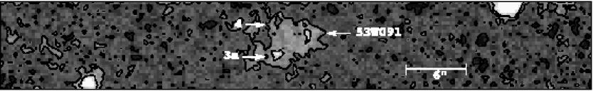
Figure 5.10: 53W091: stacked $K$-band image of August 1997 and July 1997 data.

Total integration time 5 hours 56 minutes. [4 hours 4 minutes (August) plus 1 hour 52 minutes (July).] (North is at the top, East at the left. The image has been overlaid with contours fitted for 8%, 16% and 24% of the peak intensity present.)

Two stars on our image (the star on the top right of Figure 5.10 and a brighter one in the lower slot of the focal plane mask, not shown) were identified with stars whose B1950 co-ordinates were obtained from the Digitized Sky Survey [1998]. Offsetting from these stars, the B1950 co-ordinates of the $K$-band sources were obtained and are given in Table 5.8.

Table 5.8: B1950 co-ordinates of $K$-band sources in 53W091 field.

Source	$\alpha$	$\delta$
53W091	17h 21m 17$.\!\!^{{\rm s}}$898 $\pm$ 0$.\!\!^{{\rm s}}$057	$+50\hbox{${}^{\circ}$}08\hbox{${}^{\prime}$}48\hbox{$.\!\!^{\prime\prime}$}34\pm 0\hbox{$.\!\!^{\prime\prime}$}29$
3a	17h 21m 18$.\!\!^{{\rm s}}$156 $\pm$ 0$.\!\!^{{\rm s}}$029	$+50\hbox{${}^{\circ}$}08\hbox{${}^{\prime}$}46\hbox{$.\!\!^{\prime\prime}$}34\pm 0\hbox{$.\!\!^{\prime\prime}$}57$

Key: $\alpha$: B1950 Right Ascension; $\delta$: B1950 Declination.

Spinrad et al. [1997] ask whether 3a and 53W091 together might form a system displaying the alignment effect, but note that both sources’ colours suggest they are composed of old stars, for which there is no plausible alignment mechanism. (They allow that some interaction of jets from the active nucleus with the material surrounding the galaxy may cause some appearance of filamentary structure.) The axis connecting the two objects is at a position angle of 126^∘, comparable to the radio axis at 131^∘.

It is noteworthy that the diagonal distance between 53W091 and 3a is 4^′′, the same distance as between the radio lobes in the 4.86 GHz map of Spinrad et al. [1997]. The radio positions suggest that the south-east radio lobe lies due south of 53W091 (which is the north-west partner of the $K$-band pair): we cannot definitively claim that the radio and infrared pairs are congruent, nor that the infrared source of 53W091 lies between the two radio lobes. Systematic error in registering the astrometry between the two wavebands might allow either eventuality.

Polarimetry

Polarimetry was performed on both 53W091 and on Object 3a; results for both are given in Table 5.1. Since the objects were very faint and close together, the photometry aperture was not chosen according to the method in §4.3.1, but was set to a radius of 4 pixels ($1\hbox{$.\!\!^{\prime\prime}$}1$). We also attempted to prune the frames with the greatest noise from our data and repeated the polarimetric analysis. Results for both the natural ($\natural$) and ‘despiked’ ($\flat$) data are given in Table 5.1.

There is a weak indication that Object 3a is polarised, with a 70 per cent chance of the polarisation being genuine. If there truly is polarisation at a level of 10–15%, then 30–45 per cent of the light from object 3a could be scattered, and the source could consist entirely of scattered light within the error bars. (Dust scattering and non-perpendicular electron scattering will not result in total linear polarization of the scattered light.)

Is it possible that a beam from 53W091 is being scattered by a cloud at the position of 3a? The geometry suggests that this cannot be the case, since the polarization orientation is around 140^∘, which is nearly parallel to the line connecting 3a to 53W091. If 3a were a hotspot induced by a beam emerging from 53W091, a polarization orientation nearer 30^∘ would have been expected.

The core of 53W091 itself provides no evidence for polarization, and it would be difficult to obtain results as high as the 40% which Chambers (private communication) has suggested; nevertheless, short integration times on faint objects are subject to large errors in their polarimetry, so such a result is not impossible. [James Dunlop (private communication) reports that Chambers’ integration time was not greater than three hours in total, compared to our six hours.] Our polarization orientation, interestingly, is 38^∘, nearly perpendicular to the radio axis and line to object 3a; but this is unlikely to be significant with errors of $\pm 60\hbox{${}^{\circ}$}$ on our formal measure of the polarization angle.

5.2.9 MRC 0156$-$252

Structure

Eales & Rawlings [1996] have compared radio galaxies at redshifts $z\sim 1$ and $z>2$, and find that those radio galaxies at $z>2$ have brighter absolute $V$-band magnitudes, very low Ly$\alpha/$H$\alpha$ ratios, and may be subject to strong reddening by dust. Such results might be attributed to evolution in radio galaxies, or to a selection bias for more powerful active nuclei at high redshift.

MRC 0156$-$252 has the brightest known absolute $V$-band magnitude for a radio galaxy at $z\sim 2$. The cause of its high luminosity is uncertain: it may be being viewed during an epoch of star formation, or Eales & Rawlings [1996] have suggested that the source is actually a quasar obscured by dust. Broad H$\alpha$ lines suggest that some of its light is originating in an active nucleus. McCarthy et al. [1990] earlier classified it as a radio galaxy and suggested [1993], on the basis of its red spectral energy distribution, that it was a galaxy at an advanced stage of evolution. The galaxy appears unresolved in our $K$-band image (Figure 5.11), verifying the findings of McCarthy, Persson & West [1992], who did, however, find extended structure in their visible-band images.

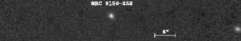
Figure 5.11: MRC 0156$-$252: stacked $K$-band image of August 1997 data.

Total integration time 3 hours 44 minutes – including one cycle of observations which was not used for our subsequent polarimetry. North is at the top, East at the left.

Polarimetry

The criterion used by L&E to select the aperture for polarimetry did not yield a unique result for this object, so photometry is given in Table 5.1 for apertures of radius 8, 10 and 12 pixels. In all cases the best point estimate of the polarization is less than 0.15 per cent; and for the 10 and 12 pixel apertures, the formal $1\sigma$ confidence interval indicates that the source is totally unpolarised.

Chapter 6 Discussion

$\star$ There is a theory which states that if ever anyone discovers exactly what the Universe is for and why it is here, it will instantly disappear and be replaced by something even more bizarre and inexplicable.
$\star$ There is another which states that this had already happened.
— Douglas Adams, The Restaurant at the End of the Universe.

The nine objects studied for this thesis project were selected for their diverse properties, and do not form any kind of statistically complete sample. No one single approach, therefore, can interpret all the new data presented in this thesis. In some cases, the published data available in the literature complements our polarimetry and enables a more detailed analysis to be made of the properties of certain targets.

One factor which can be calculated for all radio galaxies is some constraint on the contribution of the active nucleus to the total light intensity observed in the $K$-band. This is performed using some basic assumptions about the undiluted polarization of the active nucleus. Best, Longair & Röttgering [1998] have fitted radial profiles to UKIRT $K$-band images of some of our targets, and in each of these cases their figure can be used in place of our assumptions, allowing an estimate of the undiluted polarization to be made.

Spatial and spectral modelling can be performed for some interesting sources. 3C 22 and 3C 41 have had polarizations determined at other wavebands, and taken with our data the properties of the scattering medium can be modelled. The complicated morphology of sources like 3C 114 and 3C 356 invites consideration of what spatial scattering processes may be at work, and this is modelled for a simple axisymmetric scattering geometry.

We have already noted how Cimatti et al. [1993] reviewed the properties of high-redshift radio galaxies whose optical polarizations had been measured by 1993. The results of this thesis, and of the recent literature (Table 2.1) can be used to extend the parameter space in which Cimatti et al. [1993] looked for trends, and this will form the final part of our discussion.

As in the previous chapter, a series of papers by Best, Longair & Röttgering will be denoted BLR-I [1996], BLR-II [1997], and BLR-III [1998]. The dust scattering model paper of Manzini & di Serego Alighieri [1996] is abbreviated MdSA.

6.1 The Fractional Contribution of Quasar Light

As we have reviewed in Chapter 2, radio galaxies are thought to have quasar nuclei at their cores, but to be oriented such that no direct radiation from the core can reach us. Nearby radio galaxies are known to have the morphology of giant ellipticals; spectral modelling of sources at higher redshifts suggests that more distant radio galaxies, too, are dominated by old, red stars. If our target objects are typical radio galaxies, the total light received from our sources will be a combination of starlight, light from the active nucleus scattered into our line of sight, and nebular continuum emission. Direct optical power-law emission from the active nuclei of radio galaxies is normally considered to be totally obscured, but in this analysis we will also need to consider the potential contribution of such light: in some radio galaxies the obscuring material may be less efficient owing to its orientation or optical depth.

6.1.1 The dilution law for polarization

Let us denote by $\Phi_{\mathrm{W}}$, the fraction of the total flux density, ${F}_{\rm{W}}$, in a given waveband, W, which originates in the active nucleus and is scattered into our line of sight. We expect that in the visible wavebands, $\Phi_{U,B,V}$ will be a significant fraction of unity. From our observations, we wish to determine whether $\Phi_{K}$ is small, or whether a significant component of the stellar-dominated infrared also arises in the active nucleus. If we denote the flux density scattered into our line of sight from the quasar core by ${F}_{\rm{Q,W}}$, then $\Phi_{\mathrm{W}}={F}_{\rm{Q,W}}/{F}_{\rm{W}}$ — at this stage we make the assumption that there is no contribution by direct radiation from the active nucleus.

Following MdSA, we assume that only the scattered component of the light from radio galaxies is polarised. Recalling from Equation 3.6 that the degree of linear polarization is defined by $P=I_{p}/(I_{p}+I_{u})$, we define the unpolarized component to be $I_{c}$ for the scattered core light only, and $I_{c}+I_{h}$ for the scattered core light and host galaxy together. Hence defining ${P}_{\rm{Q,W}}$ as the intrinsic polarization produced by the scattering process, and ${P}_{\rm{W}}$ as the observed polarization after dilution, it follows that

$$\frac{{P}_{\rm{W}}}{{P}_{\rm{Q,W}}}=\frac{I_{p}/(I_{p}+I_{c}+I_{h})}{I_{p}/(I_{p}+I_{c})}=\frac{I_{p}+I_{c}}{I_{p}+I_{c}+I_{h}}=\frac{{F}_{\rm{Q,W}}}{{F}_{\rm{W}}}=\Phi_{\mathrm{W}}.$$ (6.1)

Therefore the fraction of the total light which is the scattered nuclear component, is equivalent to the ratio of the diluted and undiluted polarizations.

6.1.2 The dilution law in a Unification Model scattering geometry

If we know the restrictions on possible values of the intrinsic polarization ${P}_{\rm{Q,W}}$, we can use our corresponding measurements of ${P}_{\rm{W}}$ to put limits on $\Phi_{\mathrm{W}}$ for the measured sources.

The appropriate restrictions depend on the nature of the scattering centres. If the scattering centres are electrons [1989], then Thomson scattering will take place: the effects of the geometry and of the wavelength can be treated independently. The spectral energy distribution of the light scattered in a given direction is independent of the scattering angle: ${P}_{\rm{Q,W}}$ will be the same constant ${P}_{\rm{Q}}$ at all wavelengths. The degree of polarization of the scattered light is given simply by

$${P}_{\rm{Q}}=\frac{1-\cos^{2}\chi}{1+\cos^{2}\chi},$$ (6.2)

where $\chi$ is the scattering angle. For an AGN observed as a radio galaxy, we assume [1989] an orientation 45^∘ $\leq\chi\leq$ 90^∘, whence $1/3\leq{P}_{\rm{Q}}\leq 1\ \forall\$W.

The case where the scattering centres are dust grains has been modelled recently (MdSA); the fraction of the light scattered by the dust, $f_{\rm W}$, and the polarization of the scattered light, ${P}_{\rm{Q,W}}$, both depend strongly on wavelength. The exact relationship depends critically on the size distribution of the dust grains, and the amount of extinction they introduce; MdSA provide a series of graphs for the variation of $f_{\rm W}$ and ${P}_{\rm{Q,W}}$ with rest-frame wavelength 0.1 m $<\lambda_{r}<$ 1.0 m, corresponding to many different dust grain compositions and size distributions. At the redshifts of the objects in our sample, light observed in the $H$ and $J$ bands originates at rest-frame wavelengths below 1.0 m, but $K$-band light originates in the region 1.0 m $<\lambda_{r}<$ 1.15 m. To accommodate the $K$-band light within our models, we linearly extrapolated MdSA’s curves to $\lambda_{r}=1.15$ m.

In MdSA models where the smallest dust grains have a radius not less than 40 nm, ${P}_{\rm{Q,W}}$ approaches zero twice: once at a (rest frame) wavelength around 0.2 m, and again at some wavelength between 0.1 m and 0.7 m which depends critically on the dust grain size distribution. But in all cases, ${P}_{\rm{Q,W}}$ extrapolated into the 1.0 m $<\lambda_{r}<1.15$ m region gives 0.3 $<{P}_{{\rm{Q,}}K}<$ 0.5; the MdSA graphs show that the intrinsic polarizations ${P}_{{\rm{Q,}}V}$ and ${P}_{{\rm{Q,}}H}$ should be lower than ${P}_{{\rm{Q,}}K}$ for the objects where we have $V$- and $H$-band polarimetry.

6.1.3 Constraints on the nuclear component intensity of our sources

For the sources in which we have evidence of $K$-band polarization (here we will consider those with a $\geq 80\%$ probability of genuine polarization), we can hence estimate $\Phi_{K}$ under both electron and dust models. The values and upper limits are given in Table 6.1. For the dust models, we take $1/{P}_{\rm{Q,W}}=2.5\pm 0.5$; the error takes into account all dust models, and the different redshift corrections for the different galaxies, but assumes that the scattering angle is 90^∘. If the scattering angle is less, we assume that less polarization occurs (see MdSA, Figure 20), and hence $\Phi_{K}$ will be greater than our estimate. For the electron models, we multiply the observed polarization by $1/{P}_{\rm{Q,W}}=2\pm 1$; this takes into account all possible $\chi\geq 45\hbox{${}^{\circ}$}$ orientation effects.

Similarly, in all sources we can at least estimate an upper limit for the nuclear contribution contingent on our assumption of a quasar core and a $\chi\geq 45\hbox{${}^{\circ}$}$ scattering geometry. In sources which we evaluate as having a less than 80% probability of genuine polarization, we will multiply the $2\sigma$ upper limit on their measured polarizations by the $1\sigma$ upper limit on the reciprocal of the modelled intrinsic polarizations — which for both dust and electrons under the above assumptions requires a multiplication by three. These limiting values, too, are listed in Table 6.1.

Table 6.1: Percentage of $K$-band light estimated to be arising from the postulated active nucleus in our sample of radio galaxies.

Source	${P}_{\rm{K}}$	${\Phi_{K}}_{\it e}$	${\Phi_{K}}_{\it d}$	${\Phi_{K}}_{\it r}$	${\Phi_{K}}_{\it s}$
3C 22	3.3 $\pm\$1.4	7 $\pm\$4	8 $\pm\$4	37	–
3C 41	3.1 $\pm\$1.1	6 $\pm\$4	8 $\pm\$3	24	–
3C 54	5.9 $\pm\$2.6	12 $\pm\$8	15 $\pm\$7	–	–
3C 65	$<9.7$	$<29$		$<8$	1
3C 114 (T0)	11.7 $\pm\$3.0	23 $\pm\$13	29 $\pm\$10	–	–
3C 114 (T2)	5.1 $\pm\$1.7	10 $\pm\$6	13 $\pm\$5	–	–
3C 356 (T0)	9 $\pm\$5	18 $\pm\$13	23 $\pm\$13	$<14$	16
3C 356 $a$	$<41$	$\ominus$		$<14$	–
3C 356 $b$	$<24$	$<72$		$<14$	–
3C 441 a	$<10$	$<30$		$<5$	4
3C 441 c	$<24$	$<72$		–	–
3C 441 E	18 $\pm\$9	35 $\pm\$26	44 $\pm\$25	–	–
LBDS 53W091 $\flat$	$<22$	$<65$		–	–
53W091-3a $\flat$	$<46$	$\ominus$		–	–
MRC 0156$-$252 (2$.\!\!^{\prime\prime}$3)	$<10.4$	$<31$		–	–

Key: ${P}_{\rm{K}}$: measured $K$-band polarization; ${\Phi_{K}}_{\it e}$: percentage of light from quasar according to electron model; ${\Phi_{K}}_{\it d}$: percentage of light from quasar according to dust model. Depolarization from multiple scattering (both models), and shallower scattering angles (dust model only) will tend to increase $\Phi_{K}$. The $\ominus$ symbol denotes that the polarization is unconstrained since the formal upper limit exceeds 100%. ${\Phi_{K}}_{\it r}$: estimate of the percentage of light from a quasar core according to BLR-III radial profile fitting; ${\Phi_{K}}_{\it s}$: estimate of the percentage of light from a quasar core according to BLR-III flat spectrum fitting. A dash (–) indicates where no data is available from the literature. If ${P}_{\rm{K}}<80\%$ then an upper limit has been calculated as detailed in the text (§6.1.3). The last two columns may include a contribution from nuclear light arising from processes other than scattering — see text for details.

The effects of multiple scattering have been ignored for both models; multiple scattering tends to depolarise light, and so the true value of $\Phi_{K}$ under multiple scattering will again be greater than our estimate. The only physical mechanism which could cause the true $\Phi_{K}$ to be lower  than our estimate, is polarization of light in transit by selective extinction; and as we have already seen (Table 4.1), any such contribution to the polarization of our targets will be small.

6.1.4 Constraints on the nuclear polarization based on BLR-III data

Another approach to estimating the possible contribution of a quasar component is to fit the radial intensity profile of the radio galaxy with a combination of a de Vaucouleurs law and a point source. This has been done with HST  and UKIRT imaging for five of our 3C sources (BLR-III), and the fitted values or upper limits (${\Phi_{K}}_{\it r}$) are also reproduced in Table 6.1. The same paper made a further estimate of the fraction of nuclear light present by fitting the spectrum as a combination of a (nuclear) flat spectrum and an old stellar population with the spectral energy distribution of Bruzual & Charlot [1993]; again, these fractions (${\Phi_{K}}_{\it s}$) are reproduced in Table 6.1. All of the estimates of $\Phi_{K}$ are consistent with one another; the significance in individual objects will be considered below.

It should be noted, however, that BLR-III’s ‘nuclear light’ need not include only scattered light – their simple spectral model distinguishes light from an evolved stellar population but lumps everything else (scattered central engine light, the spectral profile of newly formed stars, and nebular emission) into the ‘nucleus’. Similarly the radial profile fit distinguishes only the light sources which contribute to the de Vaucouleurs structure of a normal galaxy. Our earlier definition makes $\Phi_{K}$ the fraction of the total light which is scattered nuclear light. In particular, if the active nucleus is not perfectly shielded, the nuclear light fractions derived from BLR-III’s analysis will include direct nuclear light and may therefore be higher than the $\Phi_{K}$ values derived from our $K$-band data.

In two cases (3C 65 and 3C 441 a), the BLR-III radial fitting yields upper limits which are in fact much lower than (but obviously consistent with) the upper limits estimated on the basis of our $K$-band polarimetry. Dividing the nominal $K$-band polarization by ${\Phi_{K}}_{{\it r\!,}{\mathrm{m}ax}}$ yields a nominal lower limit to the intrinsic polarization of the nucleus, namely 27% for 3C 65 and 21% for 3C 441 a; since our $K$-band polarizations are consistent with zero within their error bars, however, these nominal nuclear polarizations are of limited usefulness.

Similarly, the spectral fitting approach yielded definite values of ${\Phi_{K}}_{{\it s}}$ in these two objects; dividing the measured polarization by this light-fraction gave nominal nuclear polarizations of 215% (sic)  in 3C 65 and 26% in 3C 441 a. But the errors on the measured polarizations make any intrinsic polarization between zero and 100% possible. If the spectral fitting figure ${\Phi_{K}}_{{\it s}}=1\%$ is accurate for 3C 65, then our nominal 2.15% diluted polarization measurement for this object is clearly too high, assuming the polarization occurs only in the nuclear component of the light.

In 3C 356 (T0), we find a better-constrained case: given a spectral fit light-fraction ${\Phi_{K}}_{{\it s}}=16$%, the intrinsic nuclear polarization is ${P}_{{\rm{Q,}}K}=57\pm 31\%$ (or for radial fitting, the lower limit  nuclear polarization is 65 $\pm$ 35%). Again, the large error on our polarization measurement gives us a constraint of limited usefulness, but we might cautiously conclude (with 1$\sigma$ confidence) that the nuclear source in 3C 356 is at least 25% polarized.

The recent finding [1997] that 3C galaxies at $z\sim 1$ are 1.7 times as bright as the radio-weaker 6C/B2 galaxies in a similar sample requires that $\Phi_{K}\mathrel{\mathchoice{\vbox{\offinterlineskip\halign{\hfil$\reset@font\displaystyle#$\hfil\cr>\cr\sim\cr}}}{\vbox{\offinterlineskip\halign{\hfil$\reset@font\textstyle#$\hfil\cr>\cr\sim\cr}}}{\vbox{\offinterlineskip\halign{\hfil$\reset@font\scriptstyle#$\hfil\cr>\cr\sim\cr}}}{\vbox{\offinterlineskip\halign{\hfil$\reset@font\scriptscriptstyle#$\hfil\cr>\cr\sim\cr}}}}40\%(=7/17)$ for 3C galaxies, if the scattering of nuclear nonstellar light is responsible for the brighter $K$-band magnitudes of 3C galaxies. Most of the results presented in Table 6.1, whether based on the polarimetry of this thesis or the BLR-III data, produce $\Phi_{K}$ values which are somewhat lower. This may be indicative of some correlation between the strength of the active nucleus and the number of passively evolving stars in the galaxy, allowing the polarizations and spectral and spatial fits to produce lower $\Phi_{K}$ values, while still producing the enhanced $K$-band brightnesses measured in the most powerful (3C) radio galaxies.

6.2 Optically Compact Sources

The most obvious division which can be made in our sample of nine sources is between those whose $K$-band image is dominated by a clear source object, and those where there is a complex structure of knots or components of comparable brightness. First we consider as a group the ‘optically compact sources’, dominated by one bright object: 3C 22, 3C 41, 3C 54, 3C 65 and MRC 0156$-$252.

Among the optically compact sources, the radio galaxies 3C 22 and 3C 41 are particularly noteworthy for the compact rounded morphologies in their observed $K$-band structure. They are also prominent for having the brightest $K$-band excess over the mean locus of the $K$-$z$ Hubble plot for 3C galaxies. When BLR-III fitted radial profiles to HST  visible and UKIRT $K$-band images of eight high redshift radio galaxies, six could be modelled by a simple elliptical galaxy de Vaucouleurs profile; but in these two galaxies alone, an additional point source was required to give a good fit in the central region. These two sources also have polarization figures available in visible wavebands, data which enable simple spectral modelling to be performed for these two sources.

6.2.1 Determination of the scattering angle from the BLR-III light-fraction

The BLR-III radial profile fitting suggests that in 3C 22, the point source contributes 37% of the total $K$-band intensity, and in 3C 41, 24%; but their fitting method is known to be biased low for sources with a high point component. By simulating the effects of an additional point source, a revised estimate could be made, suggesting that 3C 22 actually had a $50^{+20}_{-10}\%$ nuclear contribution, and 3C 41’s light included $31^{+10}_{-8}\%$ from the nucleus. Flat-spectrum component fitting was not attempted in these cases.

Clearly these very high nuclear contributions are not easily reconciled with the low polarizations of order 3% which we have measured in the $K$-band, provided our model assumptions are correct. If we assume the nuclear source is obscured from direct view and has no diluting effect on the scattered light, then the intrinsic nuclear polarizations implied by our polarization and BLR-III’s fits are of the order of 10%. Such a value is too low to be consistent with a $\chi>45\hbox{${}^{\circ}$}$ scattering geometry.

If we assume a shallower scattering angle, we should also allow for the diluting effect of nuclear light which may have become visible along a direct line of sight to the nucleus. We can put a lower limit on the scattering angle by neglecting this component; if electron scattering is taking place, we can identify the limiting scattering angle. Substituting Equation 6.2 into Equation 6.1 and rearranging yields

$$\cos^{2}(\chi)=\frac{\Phi_{K}-P_{K}}{\Phi_{K}+P_{K}}.$$ (6.3)

We find that a 3.3% polarised 3C 22 with 50% of its $K$-band emission originating in a nuclear source could be scattering light at 21^∘ $\pm$ 5^∘ if the scattering medium were electrons, or could contain dust scattering light at a slightly higher angle. Similarly the figures for 3C 41 imply electron scattering at 25^∘$\pm$ 6^∘, or a correspondingly higher angle for dust.

These models suggest that these two objects are not oriented at the $\chi\geq 45\hbox{${}^{\circ}$}$ positions of radio galaxies but are being viewed ‘down the jet’. Either the direct contribution of nuclear light is weak owing to some other factor (e.g. dust obscuration) and these angles are correct; or the direct contribution is stronger, in which case the true scattering angles are somewhat higher.

Both objects are also atypical in other properties: 3C 22 appears to emit a broad line component [1995, 1995], and both 3C 22 [1993] and 3C 41 (BLR-II) exhibit radio jets, a feature rare in radio galaxies at high redshift. For these reasons, independently of the evidence of the $K$-band light fraction and polarization, it has been already suggested that these two objects may be oriented close to the threshold between radio galaxy and radio quasar properties. This is entirely consistent with the polarization which is suggesting that these objects are oriented at $\chi\sim 30\hbox{${}^{\circ}$}$ with some direct nuclear light contribution.

A further line of enquiry is open to us, since polarization measurements in other optical wavebands are available in the literature or by private communication for these two sources. These additional wavebands give a broad baseline against which models of the scattering medium can be tested.

6.2.2 Modelling the scattering medium given multiwaveband polarimetry

Where the magnitude, W, has been measured in a given waveband for which the zero-magnitude flux density is ${F}_{\rm{W0}}$, the total flux density can be calculated:

$${F}_{\rm{W}}={F}_{\rm{W0}}.10^{-0.4{\rm W}}.$$ (6.4)

The optical flux density of quasars can be modelled well by a power law of the form $C.\nu^{-\alpha}$ where $\alpha$, the ‘spectral index’, is of order unity [1997, §1.3]. Since the efficiency with which a given species of scattering centre scatters light may depend on wavelength, we denote that efficiency by $f_{\rm W}$, and the scattered quasar component can be expressed

$${F}_{\rm{Q,W}}=C.f_{\rm W}.\nu^{-\alpha}.$$ (6.5)

It will be computationally convenient to define an ‘unscaled model light ratio’, ${\phi}_{\rm{W}}$, as

$${\phi}_{\rm{W}}=\frac{f_{\rm W}.\nu^{-\alpha}}{{F}_{\rm{0W}}.10^{-0.4{\rm W}}};$$ (6.6)

then the actual model light ratio will be ${\Phi}_{{{\mathrm{W}}}}=C.{\phi}_{\rm{W}}$. There is clearly an upper limit set on $C$ by the fact that ${\Phi}_{{{\mathrm{W}}}}$ may not exceed unity in any waveband; hence $C\leq 1/{\phi}_{\rm{W}}$. Allowing for errors in the observed magnitudes, $\Delta$W, the maximum permissible value of $C$ in a model can be constrained by inspecting every relevant waveband, since the inequality must hold in all bands:

$$C_{\rm max}={\rm min}\left[\frac{{F}_{\rm{0W}}.10^{-0.4({\rm W}-\Delta{\rm W})}}{f_{\rm W}.\nu^{-\alpha}}\right],\forall\ {\rm W}.$$ (6.7)

Hence, for a given choice of scattering model, which determines the value for $\alpha$ and the form of $f_{\rm W}$, $C_{\rm max}$ is the minimum value obtained by substituting W by each wavelength observed, in turn.

Given a measurement of the magnitude of a radio galaxy, we can predict its polarization as a function of wavelength, up to a multiplicative constant. Rearranging Equation 6.1, and employing our ‘unscaled model light ratio’, we first define an ‘unscaled model polarization’ ${\Pi}_{\rm{W}}={P}_{\rm{Q,W}}.{\phi}_{\rm{W}}$, and so express our modelled polarization as:

$${P}_{\rm{W,modelled}}={P}_{\rm{Q,W}}.{\Phi}_{{W}}=C.{P}_{\rm{Q,{\mathrm{W}}}}.{\phi}_{\rm{W}}=C.{\Pi}_{\rm{W}}.$$ (6.8)

To fit a dust scattering model, we can calculate ${\Pi}_{\rm{W}}$ by obtaining $f_{\rm W}$ and ${P}_{\rm{Q,W}}$ from suitable curves in MdSA. For electron models, the wavelength-independent term $f_{\rm W}$ can be considered to have been absorbed into the multiplicative constant, $C$, while ${P}_{\rm{Q}}$, also wavelength-independent, can be assumed to be its minimum value, 1/3. We cannot separately identify $C$ and ${P}_{\rm{Q}}$; the physical constraints on these constants are $1/3\leq{P}_{\rm{Q}}\leq 1$ and $0\leq C\leq C_{\rm max}$. If ${P}_{\rm{Q}}$ is greater than the assumed 1/3, then $C$ will be correspondingly smaller.

Given a set of $N$ polarization measurements ${P}_{\rm{W}}\pm{\sigma}_{\rm{W}}$, and a corresponding set of unscaled model polarizations, ${\Pi}_{\rm{W}}\pm{\epsilon}_{\rm{W}}$, based on measured magnitudes, we can calculate the deviation of the fit:

$$\delta=\sqrt{\frac{1}{N}.\sum_{{\mathrm{W}}_{1}\ldots{\mathrm{W}}_{N}}{\frac{({P}_{\rm{W}}-C.{\Pi}_{\rm{W}})^{2}}{{\sigma}_{\rm{W}}^{2}+(C.{\epsilon}_{\rm{W}})^{2}}}}.$$ (6.9)

The best fit is that with the value of $C$ which minimizes $\delta$, subject to the physical constraint $0\leq C\leq C_{\rm max}$.

6.2.3 A model for 3C 41

The source for which we had the most data was 3C 41, with polarimetry in 3 bands: $P_{V}=9.3$ $\pm\$2.3%; $P_{H}=6.6$ $\pm\$1.6%; $P_{K}=3.1$ $\pm\$1.1 %. We attempted to fit two models; an electron model and a typical dust model with a minimum grain radius of 80 nm. To fit the models to the observed polarizations, we tested a discrete series of possible spectral indices, $-0.5\leq\alpha\leq 2$, with a step size of $1/3$. For each value of $\alpha$ we calculated the ‘unscaled polarizations’ $\Pi_{V}\pm\epsilon_{V}$, $\Pi_{H}\pm\epsilon_{H}$, $\Pi_{K}\pm\epsilon_{K}$. We then iteratively determined the best fit value of $C$ for each $\alpha$, and took as our overall best fit that combination of $\alpha$ and $C$ which gave the lowest $\delta$.

Lilly & Longair’s [1984] data shows that 3C 41, at $K=15.95$ $\pm\$0.10, is significantly brighter than the mean $K$-$z$ relationship, by about 0.6 mag. Magnitudes for 3C 41 were available in 5 bands: $J$, $H$ and $K$ [1984] and the narrow filters g and r_S [private communication]. The $H$ and $K$ values yielded direct estimates of the corresponding ‘unscaled polarizations’ $\Pi_{H}$ and $\Pi_{K}$; $\Pi_{V}$ was estimated by linear interpolation between ${\Pi}_{\rm{g}}$ and ${\Pi}_{\rm{r_{\it S}}}$.

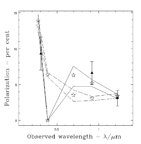
Figure 6.1: Measured and best-fit model polarizations of 3C 41 as a function of rest-frame wavelength.

Solid line: dust model, $\alpha=1.167$; dashed line: electron model, $\alpha=1.733$.

Figure 6.1 shows the measured polarizations for 3C 41 as triangles () and the magnitude-based polarization estimates, after best-fit scaling, as stars (). The lines give the error envelope on the modelled polarization (based only on the errors on the magnitudes). The solid lines correspond to the dust model, and the dashed lines to the electron model.

As can be seen from Figure 6.1, the model curves lie below the data point at $H$, but above those at $K$ and $V$. The shape of the curve depends more strongly on the measured magnitudes (and on $f_{\rm W}$ for dust) than on the spectral index, and the models for all reasonable values of $\alpha$ will have a broadly similar shape; the best fit will necessarily pass below the measured point at $H$, and above that at $V$.

Consider the electron model. Figure 6.1 shows us that the theoretical polarization curve for electron scattering is concave with respect to the origin, whereas a curve through the three data points would be convex; clearly it will not be possible to obtain a close fit for the central ($H$-band) point. Fitting the electron model curve, we found that the best fit occurred for $\alpha=1.733$, with a deviation $\delta=0.430$. From Table 6.1, we have $\Phi_{K}=6\pm 4$ per cent for 3C 41. Multiplying the polarizations observed at $H$ and $V$ by $1/{P}_{\rm{Q,W}}=2\pm 1$, we predict ${\Phi}_{{H}}=13\pm 7$ per cent, and ${\Phi}_{{V}}=19\pm 10$ per cent in these bands.

The dust model chosen as typical from MdSA was that for a cloud of spherical dust grains, with radii 250 nm $>a>$ 80 nm, with the number density per unit dust mass following an $a^{-3.5}$ law. This model produced a curve which fitted the data points very well. The best fit indicated that the optimum spectral index was $\alpha=1.167$, for which $\delta=0.177$.

This dust model was also used to estimate the proportion of scattered light at shorter wavelengths: $\Phi_{K}=8\pm 4$%, $\Phi_{H}=24\pm 6$%, and $\Phi_{V}=155\pm 38$% (sic). MdSA’s curve for polarization as a function of rest-frame wavelength predicts a 6 per cent polarization in the observed $V$-band, lower than the 9 per cent after dilution measured by Jannuzi [private communication] [1999]. This is still consistent, within error bars, as long as the true value of $\Phi_{V}$ for 3C 41 is less than, but very close to, unity; the observed $V$-band corresponds to the near-ultraviolet in the rest frame of 3C 41, and it is reasonable (MdSA) to suppose that the scattered quasar light in that band could form in excess of eighty per cent of the total light.

We noted earlier that the shape of the dust model polarization curve between 0.2 m and 0.7 m (rest frame) is very sensitive to the choice of dust grain distribution. The particular dust model chosen approaches zero polarization at a wavelength corresponding to the r_S band when redshifted into our frame. This causes the ‘well’ visible in the model polarization curve (Figure 6.1), whose presence is essential for the dust model curve to fit the data points closely.

We also considered other dust models from the selection given by MdSA. Of those which differed significantly from the ‘typical’ one considered so far, many of them will not predict polarizations in the observed $V$-band which are sufficiently high to be reconciled with the observed 9 per cent; and those which do, do not possess the deep well needed to fit the polarimetry across the spectrum. We conclude, therefore, that the best model for 3C 41 is that of an obscured quasar core with $\alpha\sim 1.2$ beaming its optical radiation into a dust cloud, although an electron model cannot be ruled out within the error bars.

6.2.4 A model for 3C 22

As we have already seen, 3C 22 is suspected of being an obscured quasar [1993, 1995]; according to data in Lilly & Longair [1984], its $K$-band magnitude ($15.67\pm 0.10$) is brighter than the mean $K$-$z$ relationship by about 0.9 mag.

For 3C 22, we have one firm polarimetry point (this thesis) and two upper limits in $V$ and $H$ [private communication] [1999]; magnitudes were available in 4 bands including $J$, $H$ and $K$ [1984], and a crude eye estimate in r [1980]. The measurements and models are shown in Figure 6.2, with the same symbols as Figure 6.1; open triangles represent upper limits. We have taken $\alpha=1$, and normalised the theoretical curves to the $K$-band data point.

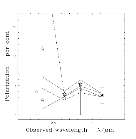
Figure 6.2: Modelled ($\alpha=1$) and measured polarizations of 3C 22 as a function of rest-frame wavelength.

Solid line: dust model; dashed line: electron model.

Here the models are inconclusive. In the observed near-infrared, both models can easily fit, with some slight scaling, within the $K$-band measurement error bars; both models suggest that about 8 per cent of the $K$-band light arises in the active nucleus (Table 6.1). The error on the observed r-band magnitude is so large that both models are consistent with the observed $V$-band upper limit of polarization.

6.2.5 Other compact sources

Manzini & di Serego Alighieri (MdSA) comment that given the range of possible dust models, ‘the wavelength dependence of polarization is not necessarily a discriminant between electron and dust scattering.’ The data available to us are insufficient to indicate whether the scattering centres in these objects are electrons or dust; it is not possible to give an unambiguous fit of the polarization curves with so few data points, although 3C 41 does seem to fit a model (MdSA) with a minimum dust radius of 80 nm particularly well, and we suggest that it does indeed consist of a quasar obscured by dust.

Since our sample of sources was selected for the variety rather than homogeneity of sources, it is difficult to come to any general conclusions on the properties of radio galaxies as a whole. There is no obvious trend of alignments, either with elongated structure of the compact optical source or the faint optical companions. $K$-band polarization may be present at any level from at least 6% down to zero. Table 6.2 indicates the different alignments (with respect to the radio jets) observed in the faint companions, optical cores, and polarizations of these objects; alignments are identified as parallel or perpendicular rather than skew if the $2\sigma$ error bars allow an aligned interpretation.

Table 6.2: Alignments in compact objects.

Source	Companions	Optical Core	Polarization
3C 22	$\perp$	$\angle$	$\perp$
3C 41	$\angle$	$\odot$	$\perp$
3C 54	$\cdot$	$\parallel$	$\parallel$
3C 65	$\parallel$	$\perp$	$\perp$
MRC 0156$-$252	$\cdot$	$\parallel$	$\circ$

Key: $\perp$: perpendicular to radio structure; $\parallel$: parallel to radio structure; $\angle$: skew to radio structure; $\cdot$ : no faint companions detected; $\odot$: optical core is round, no extended structure; $\circ$: no polarization detected.

Two of these compact sources, MRC 0156$-$252 and 3C 54, appear to be truly isolated. Both of these are extremely faint sources in the exposures available to us (Figures 4.2 and 5.11) but there is no indication of close companions of comparable brightness. BLR-II’s HST  images of the other three reveal much fainter objects in close proximity (within 5^′′), but there is no clear trend of alignment with the radio structure. 3C 22’s one companion is offset almost perpendicular to the radio jet; 3C 41 has two companions on opposite sides along an axis offset 20^∘ from the radio structure position angle; and 3C 65 has one companion lying between the optical source and its northwestern radio lobe.

There is some evidence for structure within the source galaxies. 3C 65 is slightly elongated NE-SW (BLR-II), roughly perpendicular to its radio structure; 3C 54 is extended along its radio axis [1993]; MRC 0156$-$252 is extended over 8^′′ with three knots in the $r$-band visible (rest frame ultraviolet) corresponding to its radio core and lobes, though it appears compact in $J$, $H$ and $K$ (rest frame visible bands) [1992]. Two tiny (subarcsecond) extensions are known south and west of 3C 22’s core, neither clearly related to the radio jet orientation (BLR-II).

There is no clear trend, therefore, for alignment in host galaxy structure or the positioning of companions. One skew companion is most likely a chance association of objects; two skew companions on the same axis, as seen in 3C 41, might be evidence for precession of the radio jets from the skew axis to their present position. Parallel core structure or companions suggest that the radio jet may be responsible in some way for the formation or excitation of structure along its path. Perpendicular structure could be indicative that the radio jet is orthogonal to the plane of rotation of the galaxy and its satellites. Any comprehensive model of radio galaxies clearly needs to allow, therefore, for the possibility of core structure and companions, both aligned with and orthogonal to, the large-scale radio structure.

Evidence that 3C 22 and 3C 41 may be close to the $\chi=45\hbox{${}^{\circ}$}$ boundary between radio galaxy and quasar profiles encourages us to consider the other sources in this light. The most recent radio maps of MRC 0156$-$252 [1997] do not display a marked head-tail asymmetry in radio lobe intensity at 4710 MHz or 8210 MHz, although the eastern lobe has a much greater intensity in linearly polarized 4710 MHz radiation than the core or western lobe. The formal $1\sigma$ confidence interval indicates that the source is totally unpolarised in $K$. At most, if we assume that it has radio jets perpendicular to our line of sight, 16 per cent of its $K$-band light arises in the active nucleus.

Nevertheless, it is possible that MRC 0156$-$252 is an obscured quasar [1996], and McCarthy, Persson & West [1992] note that its properties are comparable to the red quasars observed by Walsh et al. [1985]. If this is the case, we must be looking close to ‘straight down the jet’ with a shallower scattering angle for infrared light; and hence our upper limit for $\Phi_{K}$ would be weaker. The fact that McCarthy, Persson & West [1992] detect $r$-band structure on the same 8^′′ scale as the radio structure could support this, since at radio galaxy orientation, optical structure is usually less extended than radio structure, especially in the most powerful radio galaxies (BLR-I). Alternatively, if this galaxy’s high luminosity is due to star formation or direct emission from an active nucleus which is not well shielded, any scattered component might easily be diluted below a detectable level.

The five optically compact objects in our sample have been selected for their radio strength and should be presumed to share the radio emission mechanism common to all radio galaxies, unless proven otherwise. Their compact appearance gives no indication of a history of merging or recent star formation, unless the rest-frame ultraviolet elongated structure of MRC 0156$-$252 is interpreted as such. The detection of $K$-band polarization requires both the presence of a sufficiently dense scattering medium (probably situated within the host galaxy itself), and a well-shielded nucleus strong enough to yield sufficient scattered infrared light to be detectable despite dilution by the host galaxy.

The perpendicular polarizations of 3C 22, 3C 41 and (if genuine) the marginal 3C 65 are all, therefore, consistent with the Unification Hypothesis for radio galaxies. Failure to detect polarization in MRC 0156$-$252 is consistent with Unification given dilution, the absence of a suitable scattering medium, or an obscured quasar scenario. Finally, the parallel-polarized 3C 54 is the most difficult candidate to reconcile with the Unification model, requiring a special scattering geometry or possibly the presence of aligned dust grains causing polarization by transmission in the outer structure of what seems to be a quite diffuse source.

6.3 Spatial Modelling of Knotted Sources

Our four remaining sources clearly display several distinct or joined knots in their $K$-band structure: 3C 114, 3C 356, 3C 441 and 53W091. The scattering models of the Alignment Effect invite us to investigate scenarios where one knot contains an active nucleus and other knots are regions of scattering material which have intercepted a particle jet or radiation cone emerging from the central engine.

6.3.1 Polarized companions?

We have already discussed (§5.2.7) companion E to 3C 441 as a possible case of nuclear light scattered and polarized by a cloud illuminated by the central engine. Other cases giving evidence for polarization by scattering have been published recently, as the new generation of telescopes and instruments begins to make possible high-resolution imaging polarimetry of high redshift radio galaxies.

Tran et al. [1998] used the Keck I to obtain extended imaging polarimetry of 3C 265, 3C 277.2 and 3C 324. In all three cases, the polarization maps displayed bipolar fans of polarization vectors centred on the nucleus, perpendicular to the optical structure and misaligned by tens of degrees with the radio axis. Earlier structural information on one radio galaxy was obtained by di Serego Alighieri, Cimatti & Fosbury [1993]; their $V$-band polarimetry of the $z=0.567$ object $1336+020$ showed perpendicular polarization in a northern knot and in extended emission, higher than in the core.

Contour maps of the three Tran et al. [1998] sources are provided, at levels relative to the peak intensity of the central knot, and all three sources include companion objects. Little or no polarization is seen in the bright ($\sim 20$ per cent of peak) companions of 3C 277.2 and 3C 324. But in 3C 265, a faint companion object also exhibits the polarization seen in the fan – the object is a knot less than 8 per cent of peak intensity and lies beyond the extension of the $V$-band optical structure, in the same direction but unconnected with the optical core in contours down to 2 per cent of peak. Such a faint polarized knot could readily be identified with light redirected by a cloud of scattering particles.

Assuming an $\Omega_{0}=1.0,\Lambda=0$ cosmology with $H_{0}=h_{0}$ km s^-1 Mpc^-1, $h_{0}=100$, the knot in 3C 265 which lies about 9^′′ from the core, is separated from the core by about 36$h_{0}$ kpc. The extended structure of $1336+020$ of about 3^′′ corresponds to 12$h_{0}$ kpc. In comparison the 53W091 to $3a$ separation and the distance between 3C 441 a and E both correspond to approximately 16$h_{0}$ kpc. So the structure of these companion objects is of comparable scale to those in the literature.

6.3.2 Alignments in the knotted sources: an overview

The most striking feature of our small sample of four knotted sources (Table 6.3) is that in all four cases, the core and at least one other knot lie along the line of the radio structure axis. In 3C 114, three prominent knots lie on this axis and the fourth is offset perpendicular; in 3C 356, the displacement vector between the major components $a$ and $b$ lies within a few degrees of the radio axis; 3C 441 has component c closely associated with the NW radio lobe and component F fairly close to the radio axis; and 53W091 is displaced from companion 3a, again within a few degrees of the radio axis. Only 3C 441 has relatively bright companions in skew positions; and since this source seems to be in a rich field, these companions can easily be accounted for as cluster members rather than effects of the active nucleus.

Table 6.3: Alignments in knotted objects.

Source	Companions	Optical Core	Polarization
3C 114	$\parallel,\perp$	$\odot$	$\perp$ (T2), $\parallel$ (T0)
3C 356	$\parallel$	$\parallel$	$\parallel\ (a);\angle\ (b)$
3C 441	$\parallel,\perp$	$\parallel$	$\parallel$ (E); $\perp$ (a)
53W091	$\parallel$	$\angle$	$\parallel\ (3a);\perp$ (core)

Key: $\perp$: perpendicular to radio structure; $\parallel$: parallel to radio structure; $\angle$: skew to radio structure; $\odot$ : primary knot has no extended structure.

6.3.3 A conical sector model

We shall create a ‘toy model’ to help us investigate the properties of light scattered from a cloud of dust or electrons. Brown & McLean [1977] have modelled the case of axisymmetric Thomson scattering in a stellar envelope, and we can easily adapt this model to the case of scattering by an axisymmetric electron cloud in the conical region illuminated by a quasar nucleus embedded in an obscuring torus. We take an $(r,\theta,\phi)$ spherical co-ordinate system with the polar axis as the axis of the obscuring torus, and define $\mu=\cos(\theta)$. For convenience of integration we shall consider the electron cloud to have a constant number density, $n_{0}$, and to have the shape of a conical sector with boundaries $R_{1}\leq r\leq R_{2}$ and $0\leq\theta\leq\Theta_{1}$ [hence $1\geq\mu\geq\mu_{1}=\cos(\Theta_{1})$].

Brown & McLean’s [1977] treatment of the problem gives expressions for the light intensity (their Equation 5) and polarization (their Equation 16) of light scattered from an axisymmetric cloud of any number density $n(r,\mu)$ integrated over $r:0\rightarrow+\infty$ and $\mu:-1\rightarrow+1$. They define the axial inclination, $i$, as the angle between the equatorial plane of the scattering cloud (in our case, the plane of the obscuring torus) and the sky plane (the perpendicular to the line of sight from the source to Earth). In this convention, our scattering angle, $\chi$, is such that $\chi=180\hbox{${}^{\circ}$}-i$.

Substituting our special case of a constant density cloud with conical sector boundaries, we obtain:

$$I_{1}=\frac{3I_{0}\sigma_{T}n_{0}}{16}(R_{2}-R_{1})\left[(1-\mu_{1})(2+\sin^{2}i)+\frac{(1-{\mu_{1}}^{3})(2-3\sin^{2}i)}{3}\right],$$ (6.10)

and

$$\frac{1}{P}=1+2({\mathrm{c}osec}^{2}i)\left[\frac{3(1-\mu_{1})+(1-{\mu_{1}}^{3})}{3(1-\mu_{1})-3(1-{\mu_{1}}^{3})}\right];$$ (6.11)

if $I_{0}$ is the intensity (power radiated into unit solid angle) of the central source, then $I_{1}$ is the intensity of the scattered radiation; $P$ is the polarization of this radiation, and $\sigma_{T}$ is the wavelength-independent cross-section for Thomson scattering. In this formalism, a negative $P$ corresponds to polarization perpendicular to the symmetry axis.

The most striking feature of Equation 6.11 is that it is independent of the radial boundaries $R_{1},R_{2}$. It follows that for small opening angles, where a spherical cap can be approximated as a disc of constant (Cartesian) $z$, the (undiluted) polarization of any axisymmetric distribution of electrons $n(r)$ depends only on the opening angle of the illuminating aperture; we can model any axisymmetric distribution of dust $n(r)$ as the sum of scattered light from infinitessimal slices of constant density.

We will now use our toy model to investigate two scenarios: scattering from a conical region of dust stretching from the origin $(R_{1}=0)$ to some finite distance $R_{2}$; and scattering from comparable clouds at different distances from the origin.

6.3.4 A patchy cloud model

In order to use our toy model to investigate galaxy structures like that of 3C 114, we will consider what happens when similar small clouds are placed at different distances from a point source. We will consider all clouds to have the same volume, $V$, the same diameter, $w$, and the same fixed particle density, $n$. Further, for ease of integration, we will consider all clouds to be placed on the axis, and bounded by radial lines forming conical surfaces, and by spherical caps.

Let us consider a cloud which subtends some half-angle $\Theta_{1}$ and extends from $R_{1}$ to $R_{1}+\Delta R$. Now the width of this cloud we can take as the linear distance subtended by the spherical cap at $R_{1}+\Delta R/2$, viz.

$$w=2\sin(\Theta_{1}).(R_{1}+\Delta R/2);$$ (6.12)

the volume is obtained by the trivial integration of $r^{2}\sin\theta\,dr\,d\theta\,d\phi$ over $(R_{1},R_{1}+\Delta R)$ in $r$, 0 to $\Theta_{1}$ in $\theta$, and 0 to $2\pi$ in $\phi$, whence

$$V=(2\pi/3).(1-\cos\Theta_{1}).[(R_{1}+\Delta R)^{3}-{R_{1}}^{3}].$$ (6.13)

For given $w$, $V$ and distance from the illuminating source, $R_{1}$, the appropriate opening angle $\Theta_{1}$ and radial thickness $\Delta R$ can easily be calculated. Trial and error revealed that with $V=6.6$ and $w=2$, the calculated $\Delta R$ values were also of order 2 at various radii $R_{1}$, yielding a model cloud about as broad as it is deep. Such a quasi-symmetric cloud seems the most appropriate for a toy model mimicking fairly symmetrical knots in galaxies. The different dimensions of this conical sector cloud at differing radii are given in Table 6.4.

Table 6.4: Dimensions of a conical sector of fixed volume and width.

$R_{1}$	$\Delta R$	$\Theta_{1}$	$\mu_{1}$
1	1.81	31.68	0.851
2	1.97	19.58	0.942
3	2.02	14.43	0.968
4	2.05	11.48	0.980
5	2.07	9.54	0.986
6	2.08	8.17	0.990
7	2.08	7.14	0.992

Key: The dimensions above are for a conical sector bounded by spherical caps at $R_{1}$ and $R_{1}+\Delta R$, and a conical surface subtending a semi-vertical angle of $\Theta_{1}$, such that the volume enclosed is 6.6 units and the diameter of the disc bounding the spherical cap at $R_{1}+\Delta R/2$ is 2 units. We define $\mu_{1}=\cos(\Theta_{1})$.

By substituting the boundaries for such a cloud into Equations 6.10 and 6.11, we can immediately obtain the polarization and relative intensity of the light scattered by similar clouds at different densities. The undiluted  polarization is, in fact, independent of both the cloud density and the intensity of the illuminating source. The polarizations and intensities (relative to the $R=1$ case) are given in Table 6.5. It is also useful to calculate the surface brightness, $B=I_{1}/A$: approximating the side-on profile of the cloud as a sector subtending half-angle $\Theta_{1}$, the area bounded between $R_{1}$ and $R_{1}+\Delta R$ is $A=2\Theta_{1}[(R_{1}+\Delta R)^{2}-{R_{1}}^{2}]$.

Table 6.5: Polarization and intensity of light scattered by a small cloud at various distances from an illuminating nucleus.

$R_{1}$	$P$(%)	$I_{r}$(%)	$B_{r}$(%)	$P_{r}$(%)
1	73.6	100.0	100.0	100.0
2	89.0	40.6	38.5	55.7
3	93.9	22.5	20.9	34.0
4	96.0	14.4	13.2	22.6
5	97.3	10.0	9.1	16.1
6	98.0	7.3	6.7	12.0
7	98.5	5.6	5.1	9.3

Key: $R_{1}$: Distance of inner edge of cloud from illuminating nucleus; $P$: polarization of light scattered by cloud (always perpendicular to the nucleus-cloud axis in the cases above) (%); $I_{r}$: relative intensity $I_{1}(R_{1})/I_{1}(1)$ (%); $B_{r}$: relative surface intensity $B(R_{1})/B(1)$ (%); $P_{r}$: relative diluted polarization $P_{d}(R_{1})/P_{d}(1)$ (%).

It is evident from Table 6.5 that clouds of a given size lying further from their source of illumination are more strongly polarized, but the intensity of the polarized light is diminished. Obviously at greater distances, the angle (and hence fraction of the source emission) subtended by the cloud is smaller, but the beam entering the cloud is more collimated and hence there is less cancellation of polarization from light being scattered in opposite senses.

The toy model does not require that the illuminating source be shielded, only that it be pointlike; so a scattering cloud illuminated by an external small non-AGN source (e.g. a star cluster) would also produce polarised light in the manner of this model. If the scattering cloud’s only source of light is the external illumination, it is clearly not possible to obtain a structure of knots of similar brightness at different distances from the nucleus, since the relative intensity (and surface intensity) drop off so rapidly with distance. Where the intensity of the intrinsic emission of the knot, $I_{k}$, is much greater than that of the scattered light, the polarization of the diluted light can be approximated as $P_{d}=P.I_{1}/I_{k}$, and the values of $P_{d}$ relative to that at $R_{1}=1$ (since the absolute value depends on the knot’s intrinsic brightness) are also tabulated in Table 6.5.

Is a scattering model adequate, therefore, to account for the knotted structures seen in many high-redshift radio galaxies? The central engine, by definition, must be many times brighter than any scattering clouds shining purely by scattering some small portion of its output; but if the nucleus is well-shielded then the residual starlight of the host galaxy might be of comparable brightness to a knot of scattered light. If there are multiple knots, those at greater distances from the nucleus should be much fainter, following Table 6.5, unless they contain denser clouds of scattering material than the nearer clouds. Knots offset more than 45^∘ from the radio axis ought to be shielded from the central engine by its obscuring torus; the light of such knots cannot easily be attributed to scattering.

6.3.5 A continuous cloud model

Another useful model to examine is that of a scattering cloud bounded by $0\leq r\leq R_{1}$ and $0\leq\theta\leq\Theta_{1}$. This case can model an AGN whose conical region of illumination is filled with scattering particles close to the active nucleus. In a canonical model with $\Theta_{1}=45\hbox{${}^{\circ}$}$ where the particles fill the opening angle of the central engine, then $P=53.3\%$. The undiluted polarizations owing to cones filled at other opening angles are given in Table 6.6. Again, the undiluted polarizations are perpendicular to the conical axis and independent of the radial extent of the scattering region. One important consequence of this model is that any measurement implying an undiluted polarization much greater than 50% is indicative of a scattering medium subtending an angle smaller than the whole 45^∘ illumination zone.

Table 6.6: Polarization of scattering cones filled to various opening angles.

$\Theta_{1}$	5	10	15	20	25	30	35	40	45	50	55
$P$	99.2	97.0	93.4	88.5	82.6	75.9	68.7	61.1	53.3	45.6	38.2

Key: $\Theta_{1}$: opening angle of scattering cone (^∘); $P$: polarization due to scattering in this cone (%).

6.3.6 3C 114

We turn first to 3C 114, with three knots lying along the radio jet and one offset perpendicularly (Figure 5.5). In this source, the ‘knee’ knot (T2) is presumably part of the parallel aligned structure, and its polarization is roughly perpendicular to the radio jet, as expected if some scattering process is at work inside the knot, perhaps a region of dust in the scattering cone as discussed immediately above. The rest of the structure, however, is difficult to interpret in terms of a scattering model. We have no polarimetry on the knots T3 or T4, but if T2 contains the central engine, T4 is brighter than T3 though it lies beyond T3. Clearly the light from T4 cannot primarily be scattered light and some other mechanism must be at work (e.g. jet induced star formation) to produce the Alignment Effect in this object.

When polarimetry is performed over the whole aperture, including the perpendicular knot T1, the overall polarization seems parallel  to the radio jet — i.e. perpendicular to the axis connecting this anomalous knot to the main structure. Is this indicative of some scattering mechanism perpendicular to the main radio structure? It is difficult to conceive of a mechanism which allows a brilliant central engine to emit light in two perpendicular directions without also leaking such light towards Earth; yet the morphology (and indeed the high polarization which implies that any dilution is limited) do not suggest that we are seeing a central engine directly in T2. Could T1 be a chance alignment or a satellite galaxy? This would explain its presence but not the overall parallel polarization. The brightness of the knots in 3C 114 make it a prime candidate for spectroscopy or spectropolarimetry, which would shed more light on the chemistry and light emission mechanisms at work in each of the knots.

6.3.7 3C 356

We have already reviewed the structure of 3C 356 (§5.2.6) and noted how the SE radio core $b$ has been proposed as the central engine with component $a$ interacting with its jet [1994, 1990]. More recent imaging (BLR-III) and spectropolarimetry [1997], however, now point towards $a$ as being the more likely host of the active nucleus. Broad lines are clearly visible in the polarised spectrum of $a$, which itself is now known to have two components (BLR-II); two components are aligned along the $a-b$ axis with the component nearer $b$ providing 60% of the total emission from $a$. The Keck spectropolarimetry unequivocally demonstrates the presence of a polarized component strong in the near-ultraviolet and declining into the green; our $K$-band polarimetry cannot identify this polarized component in the near-infrared, suggesting that nebular emission and starlight are dominating this waveband.

The weight of evidence in the more recent literature, though not conclusive, indicates $a$ as the more likely host of the 3C radio source, though in this case $b$ seems to be a flat-spectrum radio galaxy in its own right. Comparison of the spectra of $a$ and $b$ presented by Cimatti et al. [1997] does not suggest that $b$’s main source of light is scattering from $a$’s emission, nor is the polarization in $b$ high; they also show that the polarization in $a$ can be modelled both by dust and by electron scattering. The high $(\sim 15\%)$ polarization present in the ultraviolet shows that scattered light must form a large proportion of the light from $a$ at these frequencies, and Cimatti et al. [1997] estimate that at 280 nm, 50 $\pm\$15% of the total flux from $a$ is scattered light, and the intrinsic undiluted polarization is 21 $\pm\$7%. Our $K$-band data can only add to this the knowledge that the diluting component is much stronger in the infrared.

6.3.8 3C 441

Analysis of 3C 441 is complicated by the richness of the field in which it lies; without knowledge of the redshifts of all the objects, and hence of which could be true neighbours to the radio core, any interpretation must be tentative. Object E is known to be much fainter than the presumed active nucleus in $K$ (this thesis) and in $I$ and [O ii] [1996]. This is consistent with a scattered light hypothesis and it is highly plausible that companion E to 3C 441 is an illuminated object scattering light in the manner of the extended structure seen in 3C 265 and $1336+020$, pending confirmation of its redshift — though it must be noted that the result for E does have a ten percent chance of being a noise-induced spurious result.

6.3.9 LBDS 53W091

Unlike the other objects in this thesis, LBDS 53W091 was chosen on the basis of the weakness  of its radio emission. Its apparent age and redshift are hard to reconcile and the reported 40% polarization did not help to clarify the picture. We have ruled out a $K$-band polarization of that order; most of the discussion of this galaxy’s peculiar properties can be found in §5.2.8 and in more detail in Leyshon, Dunlop & Eales [1999].

We have seen how radio-weak galaxies only display the Alignment Effect over small scales, up to about 15 kpc [1999b]; the separation between 53W091 and companion 3a is of this order (16$h_{0}$ kpc) and so its good alignment is in keeping with what is known for 7C galaxies. We have seen (§5.2.8), however, that the polarization in 3a cannot be reconciled with a scattering model; and the result for 3a is too tentative to warrant developing alternative models.

6.4 Radio Galaxy Trends: The Big Picture

The data presented in this thesis represents the first $K$-band polarimetry of high redshift radio galaxies; that is, the measurements are the first on record for the rest frame near-infrared (0.7–1.3 m) polarizations of radio galaxies significantly less evolved than the local universe. The results can be compared with the infrared properties of nearby radio galaxies and with the visible-light properties of high redshift objects (§2.3.2) — always bearing in mind that our sample of nine diverse objects is of limited statistical significance.

Some nearby radio galaxies (Cen A, IC 5063, 3C 234) have been observed in the $K$-band (§2.3.2) and found to have polarizations of order 10%, oriented perpendicular to the radio jet. In these cases, it seems that the standard scattering hypothesis is the best explanation. 3C 233.1 is 5% polarized in $K$ but less than 0.5% in the visible, suggesting that dust extinction may reduce the contribution of visible scattered light. Our sources are being observed at rest-frame wavelengths somewhat shorter than the 2.2 m $K$-band, so if 3C 233.1 were used as a benchmark, we might expect perpendicular polarizations somewhat lower than 5%. In fact our measurements range between zero and 20%, all in the ‘ballpark’ defined by these earlier $K$-band observations.

We have noted (§2.3.3) how Cimatti et al. [1993] analyzed the properties of 42 radio galaxies at $z\geq 0.1$ and searched for trends with both the observed polarization and their estimate of the underlying nuclear polarization. All their conclusions were based on light emitted at rest frame wavelengths between 0.2 m and 0.7 m, so the observations of this thesis do not overlap in $\lambda_{r}$ with theirs. Nevertheless, it is valuable to try to interpret our results in the context of their trends analysis.

Cimatti et al. [1993] found that a good rule of thumb was that radio galaxies at $z>0.6$ were polarized above 8% and those at lower redshift, less than 7%. All of our sources lie at $z>0.6$, but some are certainly polarized below 7% in $K$-band, the firmest results being the unpolarized MRC 0156$-$252 and the 3% polarized 3C 22 and 3C 41. Jannuzi [private communication] reports that 3C 22 is no more than 5% polarized in the $V$-band; 3C 41 fulfills the rule of thumb in $V$ but not in $H$. The rule, however, is a rule for radio galaxies, so if these objects are actually obscured quasars the rule is not applicable to them. Spectropolarimetry for 3C 356 $a$ [1997] shows the rule satisfied in this source at 0.2 m but not at 0.4 m, while our results indicate that it probably obeys the rule at 1.1 m. The handy rule of thumb, therefore, must be used with the caveat that it applies only to light emitted at visible/ultraviolet rest wavelengths.

There is also a rule of thumb based on general results about alignments. Radio galaxies with $z>0.6$ and $P>5\%$ were always found to have perpendicular polarizations. Again, this is not found to carry into the $K$-band, since 3C 54’s polarization is parallel, and 3C 114 is ambiguous depending on which knots are included. Neither can we sustain the rule that if a radio galaxy polarization is in parallel alignment, the polarization is always lower than 5%: the same two objects and 3C 356 may all have higher parallel polarizations.

Except for 53W091, all the objects in our sample are very radio loud; all lie at high redshift. They would therefore be expected to display a clear Alignment Effect in the visible (§2.3.1) and at least a marginal effect in the infrared. In fact the knotted sources (Table 6.3) do display parallel aligned structures, though some (most strikingly 3C 114) also have knots in perpendicular alignment — a feature not unknown in nearby radio galaxies [1997]. Discerning alignments present in compact objects (Table 6.2) is, by definition, more difficult, and no clear trend is apparent in our five compact sources. Clearly bright knots, where present, dominate any analysis of alignments and structure, whereas the slight extensions or faint companions of radio galaxies may not be related to the mechanism which sometimes causes aligned or perpendicular knots.

Chapter 7 Conclusions

It seemed to me that in one of my innumerable essays, here and elsewhere, I had expressed a certain gladness at living in a century in which we finally got the basis of the Universe straight.
— Isaac Asimov, The Relativity of Wrong.

The work contained in this thesis has pushed forward scientific knowledge on two fronts: the practice of astronomical polarimetry, and our knowledge of the $K$-band polarization properties of radio galaxies. As always in science, new results reveal to us how little we know about the Universe at large and suggest future avenues of exploration. It is clear that there is great room for improvement in the polarimetric analysis software available to the astronomical community, and some recommendations are made here on functions which should be included in any comprehensive analysis package of the future.

Our sample of targets was selected for its diversity and provides a snapshot of some interesting objects; even so, some of these provide marginal results over the maximum realistic integration time on a world-class infrared telescope. Today, we can only dream of taking a sample large enough to yield good statistics: the number of objects and the integration times which would be required conspire to place such a project in the realms of spaceborne infrared telescopes, Keck-size telescopes, or weeks of dedicated observing time. In the meantime, individual $K$-band objects will surely be subjected to polarimetric analysis, and it is possible to give some pointers for properties to look out for.

7.1 Requirements for a Comprehensive Polarimetric Software Package

The software currently available for polarimetric analysis (aaopol from the Anglo-Australian Observatory and polpack from Starlink ) concentrates on the generation of ‘vector maps’ illustrating the polarization of different parts of an image by means of arrows of appropriate length and orientation. Such software is fine for imaging polarimetry where there is a high-quality signal, but is inadequate to deal with pioneering research where the signal-to-noise ratio is low. The experience gained in performing the analysis for this thesis suggests that a future comprehensive polarimetry package should include the following features for two-channel Wollaston prism systems with a waveplate rotating in 22.5^∘ steps.

7.1.1 Generation of the Stokes Parameters

An imaging polarimetry package would normally function as an accessory to an imaging photometry system. It would be necessary to define one or more polarimetry apertures (a whole object, a series of knots, etc.) and define the binning resolution (the whole aperture, individual pixels, or some intermediate level). It should be possible to define a list of input images (possibly several for each waveplate) and tag each of them with the orientation of the waveplate used for that exposure; the orientation, $\eta_{0}$, of the reference axis of the waveplate system should also be noted. It would be desirable to provide automatic and manual facilities for registering the waveplate images rather than assuming perfect alignment.

Having defined the sampling apertures and resolution, the software should be capable of calling the photometry package, accepting the returned photometry data, and converting the results to absolute Stokes Parameters (with errors) relative to the waveplate reference axis. The reference angle and Stokes parameters for each pixel bin of each source on each image should be stored in a file for further analysis. This part of the software should implement Steps 1 to 7 of Chapter 3.

7.1.2 Stokes Parameter analysis routines

The nucleus of a polarimetry package should be a versatile system for performing analysis on sets of Stokes Parameters, absolute or normalized, derived from the photometry procedure detailed above, or directly entered from the literature. Among the analysis routines available should be the following:

1. Derive the optimal estimates of the normalized Stokes Parameters from the absolute Stokes Parameters, following (i) Steps 9 to 12, or (ii) the iterative method of §3.13.

2. Estimate the probability that the true polarization of a bin is zero/non-zero using any of three methods: (i) the absolute Stokes Parameter confidence interval test (Step 8), (ii) the polarization debiasing test (Step 16) and (iii) the residual method (§3.13).

3. Convert normalized Stokes parameters to percentage polarization (Steps 13 to 15) and orientation (Steps 17 and 18) format, providing point estimates and/or confidence intervals.

4. Convert data in the form of percentage polarization and orientation into Stokes Parameter form, both for ‘debiased’ polarizations and non-debiased crude estimates of the percentage polarization. (Such a function allows rapid conversion of data from the literature into a form comparable with other data.)

5. Test two sets of Stokes parameters for consistency with one another (for studying temporal variability etc.).

6. Convert Stokes Parameters from a given reference frame to a standard frame where the axis points North. (Working in the instrumental frame is best as the errors on the two channels are independent of one another; but standard orientation may be needed if data from two telescopes with different reference axes are to be combined.)

7. Combine two sets of normalized Stokes parameters. (Combining two sets of absolute Stokes Parameters is a trivial extension of function (a) unless the two reference axes are misaligned.)

A software package capable of performing all these analyses would be a powerful tool enabling the rigorous analysis of new polarimetric data and efficient comparison with the existing literature. Ideally the software should be able to output the debiased data in a form compatible with existing software for displaying polarization vector maps. Limited by the shot noise inherent in photometry of faint sources, and providing optimal estimates, such software would yield the most accurate estimates of true polarizations theoretically possible, and these recommendations are commended to astronomical programmers for their consideration.

7.2 A Summary of the Properties of Our Sample

We have taken $K$-band polarimetry for seven 3CR radio galaxies, and found a diverse range of results. Out of our seven sources, two (3C 65 and 3C 441) display no evidence for polarization (though a companion to 3C 441 may be polarised). For the sources which do display some evidence of polarization, we have estimated the fraction of observed $K$-band light which originated in the active nucleus (Table 6.1). Most of our findings are lower than the $\Phi_{K}\mathrel{\mathchoice{\vbox{\offinterlineskip\halign{\hfil$\reset@font\displaystyle#$\hfil\cr>\cr\sim\cr}}}{\vbox{\offinterlineskip\halign{\hfil$\reset@font\textstyle#$\hfil\cr>\cr\sim\cr}}}{\vbox{\offinterlineskip\halign{\hfil$\reset@font\scriptstyle#$\hfil\cr>\cr\sim\cr}}}{\vbox{\offinterlineskip\halign{\hfil$\reset@font\scriptscriptstyle#$\hfil\cr>\cr\sim\cr}}}}40\%$ suggested by the recent findings of Eales et al. [1997] but are consistent with the hypothesis that radio galaxies consist of quasar nuclei embedded in giant elliptical galaxies.

All of the galaxies which appear to be polarised have large errors on the orientation of their $E$-vectors; hence any apparent alignment effects are suggestive rather than definitive. But with this caveat, we note that two sources (3C 54 and 3C 114) have high polarizations oriented in roughly parallel alignment with the radio axis and extension of the optical structure — i.e.  in the opposite sense to the perpendicular alignment expected under a simple scattering model.

The compact galaxies 3C 22 and 3C 41 display significant polarizations of around 3% with a polarization alignment perpendicular to their radio axes; both appear in the $K$-band as pointlike objects. We suggest, therefore, that in these objects, infrared light from a quasar core is being scattered into our line of sight, and forms a significant part of the total $K$-band flux received from these sources; both objects may be inclined close to the $\chi\sim 45\hbox{${}^{\circ}$}$ ‘boundary’ between quasar and radio galaxy properties.

In the case of MRC 0156$-$252, which lies beyond a virtually dust-free part of our own Galaxy, we can be reasonably certain that this radio galaxy is not polarised, and the $K$-band light has not been scattered before reaching us. If some of the $K$-band light has originated in the active nucleus, its contribution should be smaller than at visible wavelengths [1996]; this being the case, subtraction of our image or a synthetic symmetrical galaxy could well reveal the structure of the active component at visible wavelengths, given the visible structure observed by McCarthy et al. [1992]. It is possible that this galaxy, like 3C 22 and 3C 41, is an obscured quasar at an intermediate orientation.

In LBDS 53W091, we can rule out the contribution of an active nucleus to providing more than $\sim 25$ per cent of the observed light. The majority of its $K$-band light, therefore, must be presumed to be due to its stellar population, and its $R-K$ colour remains consistent with an age in the range $2.5-3$ Gyr. The nature of its companion object $3a$, possibly polarised and of unclear physical relationship with 53W091, warrants further investigation.

In 3C 441, the polarization from object E may indicate that E is scattering light from a (whose identification as the central engine would thus be vindicated); the orientation of E’s polarization would not be consistent with the source being located within E or F and emitting jets at $\sim 145\hbox{${}^{\circ}$}$. Therefore, we favour the traditional identification of the central engine with a. Although this object was observed at two epochs, the observational errors cannot rule in or out temporal variability in polarization over a two year period.

It is noteworthy that when radial profile or spectral fitting estimates [1998] are combined with our $K$-band data (§6.1.4), there are hints that the true $K$-band nuclear polarizations of several sources (3C 65, 3C 356, 3C 441 a) are of the order of 25%. The measurement errors and uncertainties in the derivation mean that these figures are no more than indicative; but following Enrico Fermi’s rule of thumb that in a sufficiently complicated problem, uncertain contributions tend to cancel out each other, this can be taken as a very tentative indication for $K$-band nuclear polarizations of order 25% in radio galaxies.

Polarimetry of faint objects requires long integration times. The observing time available has permitted us to rule out the existence of very high polarizations in many of the objects studied, at least for light emitted along the line of sight to Earth. It would still be possible for light emitted in other directions from these objects to be polarised. ‘Polarization’ mentioned in these conclusions should be understood in the restricted sense of light leaving the source in the direction of Earth. Under the Unification Model, radio galaxies (a class of AGN assumed to be oriented with their jets perpendicular to that line of sight) would be more likely to display polarization originating in scattering or synchrotron radiation in the light travelling Earthwards than in directions closer to the jet.

7.3 Recommendations for Future $K$-band Radio Galaxy Polarimetry

Interpreting polarization measurements is intimately linked with understanding the morphology of the knots or extensions which accompany a radio source. It is a distinct advantage to study sources in which the redshifts of the companion objects are known, so that chance alignments can be ruled out, and true near-neighbours can be identified as such. Where redshifts are not available and the source lies in a rich field, multifibre spectroscopy of the sources should be scheduled. Then, if an imaging polarization measurement suggests that a knot may be scattering nuclear light, the AGN spectrum could be scaled and subtracted from that of the knot.

The spectral and spatial profile fitting methods of Best, Longair & Röttgering [1998] greatly complement the data available from polarimetry, since stronger limits can be placed on the nuclear polarizations if the fraction of the light due to stars can be independently identified. There would be a distinct advantage in performing polarimetry on the other objects already analysed by them, or applying their analysis (de Vaucouleurs fitting could be done on the imaging polarimetry images in good seeing) to stacked polarimetric images.

Polarimetry is a cheap ‘overhead’ which could be seriously considered whenever imaging or photometry is being carried out on a radio galaxy whose linear extent is such that it can easily be viewed through a focal plane mask. Polarimetry complements mosaicing by spreading the image over the pixels available, and local effects are cancelled out when the waveplate is rotated through 45^∘. Combining the two slits for imaging purposes can be integrated into the mosaicing process. The photon rate in each channel is 50% of that which would be achieved with no Wollaston prism (for both source and sky noise), so doubling the time per exposure would produce noise at the same level per integration as using the system without the Wollaston prism. In the same spirit, applying a Wollaston prism before a grating or multifibre spectroscopy system allows spectropolarimetry AND spectroscopy of a given quality to be done in just twice the time of spectroscopy alone.

Sources in which there is evidence for scattered light from a distinct knot – such as 3C 441 – are prime candidates for spectropolarimetry to be applied to their distinct knots. Tracing the nuclear spectrum in the polarized spectrum of the knot would confirm the scattered light hypothesis.

Spectropolarimetry should also be applied to sources in which there are indications of parallel polarization, such as 3C 114, 3C 54 and 53W091 3a. Only low parallel polarizations can be produced by flattened scattering discs, and untangling the spectrum of the parallel polarized component would give a better hint at what is taking place in such sources.

Sources in which their are indications of a skew Alignment Effect with infrared structure 10^∘–20^∘ out of line with visible structures (§2.3.1) are also particularly interesting targets for further study, as are those where optical polarization is somewhat misaligned with radio structure (§2.1). It would be a valuable exercise to perform a full literature review and observing campaign to compare the polarization orientation with the position angles determined for structure in the radio, near-infrared, visible and near-ultraviolet bands for every AGN with a published optical polarization. Understanding the wavelength-dependence of the skew alignment would probe the mechanism at work in these objects.

Finally, all polarimetric studies must be realistic about the time required to get a useful result. Low polarizations are harder to isolate than high ones; we spent more than an hour on 3C 22 and nearly two on 3C 41, our brightest sources; and the errors on these are still quite large. Six hours on the faint 53W091 has refuted any suggestion of 40% levels of polarization but cannot give a definitive answer on the presence or absence of lower levels. The author looks forward to the days when larger telescope mirrors, parallel use of Wollaston prisms and imaging spectroscopy allow the radio galaxy trends survey of Cimatti et al. [1993] to be extended to $K$-band observations, and the true contribution of scattered $K$-band light to the properties of high-redshift radio galaxies will be known.

Chapter A Minimum Theoretical Errors in Stokes Parameters

The recent work of Sánchez Almeida [1995], and of Maronna, Feinstein & Clocchiatti [1992], considers the ideal case of polarimetry limited only by the shot noise intrinsic to quantized light. For completeness their results are presented here in the notation of this thesis, and extended slightly in the case of normalised Stokes Parameters. (See Chapter 3 for definitions of the Stokes Parameters.) This treatment also considers which estimators are optimal for estimating Stokes Parameters, and the consequences of binning the photon counts.

A.1 Light Intensity as a Poissonian Quantity

Consider a quasimonochromatic beam of light of intensity $I$, where the units of $I$ are photons per second. In a time interval $\tau$, the number of photons expected to arrive is $\lambda=I\tau$. As bosons, there will be some correlation between the arrival of individual photons, but this effect is negligible at optical wavelengths, and we can assume that the arrival of photons can be characterised by a Poisson distribution [1987, Ch. 2]. The number of photons actually arriving is hence a Poissonian random variable $X$, such that

$$P(X=x)=\frac{e^{-\lambda}\lambda^{x}}{x!}.$$ (A.1)

In the remainder of this appendix we will speak of such a Poisson distribution as having an intensity $I$, indicating that the mean of the distribution is $\lambda=I\tau$ for some arbitrary integration time $\tau$.

A.1.1 Combining beams

Theorem 1

Combining two beams of light of intensity $I_{1}$ and $I_{2}$ produces a Poissonian beam of intensity $I=I_{1}+I_{2}$.

If the beams yield $\lambda_{1}\tau$ and $\lambda_{2}\tau$ photons respectively in the obvious notation, then

$$P(X=x)=\sum_{i=0}^{x}P(X_{1}=i).P(X_{2}=x-i)=\sum_{i=0}^{x}\frac{e^{-\lambda_{1}}{\lambda_{1}}^{i}}{i!}.\frac{e^{-\lambda_{2}}{\lambda_{2}}^{x-i}}{(x-i)!}$$ (A.2)

and factorizing out the exponential term,

$$P(X=x)=e^{-(\lambda_{1}+\lambda_{2})}\sum_{i=0}^{x}\frac{{\lambda_{1}}^{i}{\lambda_{2}}^{x-i}}{i!(x-i)!}.$$ (A.3)

Anticipating the result, we substitute $\lambda=\lambda_{1}+\lambda_{2}$ into Equation A.1 and use the binomial expansion to obtain

$$P(X=x)=\frac{e^{-(\lambda_{1}+\lambda_{2})}}{x!}(\lambda_{1}+\lambda_{2})^{x}=\frac{e^{-(\lambda_{1}+\lambda_{2})}}{x!}\sum_{j=0}^{x}{\lambda_{1}}^{j}{\lambda_{2}}^{x-j}\frac{x!}{j!(x-j)!}.$$ (A.4)

Since the factors of $x!$ cancel and the indices $i$ and $j$ are summed over, then Equation A.3 is identical to Equation A.4 and the combined beams produce a Poisson distribution of mean intensity $I_{1}+I_{2}$. QED.

Consequence 1

It follows that when Poissonian light from two sources is combined – e.g. light from a pair of stars, or from a host galaxy and an active nucleus – the resultant beam is also a Poissonian.

A.1.2 Attenuating beams

Theorem 2

Passing light of intensity $I$ through a filter which passes a fraction $f$ of the photons results in a Poissonian beam of intensity $fI$.

The number of photons arriving at the filter follows a Poisson distribution for intensity $I$, so $X$ photons arrive at the filter. There is a binomial distribution such that $W$ photons penetrate the filter given that $X$ arrive, where

$$P(W=w\,|\,X)=\frac{X!}{w!(X-w)!}f^{w}(1-f)^{(X-w)}.$$ (A.5)

Overall the probability that $w$ arrive and penetrate is given by

$$P(W=w)=\sum_{x=w}^{\infty}P(X=x).\frac{x!}{w!(x-w)!}f^{w}(1-f)^{(x-w)}.$$ (A.6)

Making the substitution $k=x-w$ and expanding $P(X=x)$ from Equation A.1, we obtain

$$P(W=w)=\sum_{k=0}^{\infty}\frac{e^{-\lambda}\lambda^{k+w}}{x!}.\frac{x!}{w!k!}f^{w}(1-f)^{k}$$ (A.7)

and the $x!$ terms cancel. We take out the terms in $w$ and obtain

$$P(W=w)=\frac{(f\lambda)^{w}}{w!}.\left[e^{-\lambda}\sum_{k=0}^{\infty}\frac{\lambda^{k}}{k!}(1-f)^{k}\right].$$ (A.8)

To complete the proof we must show that the term in square brackets is equivalent to $e^{-f\lambda}$. So, let the term in square brackets be denoted $G$. Expressing $e^{-\lambda}$ as a series, we have

$$G=\sum_{j=0}^{\infty}\frac{(-\lambda)^{j}}{j!}\sum_{k=0}^{\infty}\frac{\lambda^{k}}{k!}(1-f)^{k}.$$ (A.9)

We can express the double series as a single series if we group together terms of the same power of $\lambda$:

$$G=\sum_{i=0}^{\infty}\lambda^{i}\left[\sum_{j=0}^{i}\frac{(-1)^{j}}{j!}\frac{(1-f)^{i-j}}{(i-j)!}\right].$$ (A.10)

We now let $h=1-f$, and recast this as

$$G=\sum_{i=0}^{\infty}\lambda^{i}\left[\sum_{j=0}^{i}\frac{(-1)^{j}}{j!}\frac{h^{i-j}}{(i-j)!}\right],$$ (A.11)

where we recognise the square bracket as $1/i!$ times the binomial expansion

$$(h-1)^{i}=\sum_{j=0}^{i}\frac{(-1)^{j}h^{i-j}i!}{j!(i-j)!}.$$ (A.12)

Thus Equation A.10 can be simplified to

$$G=\sum_{i=0}^{\infty}\frac{\lambda^{i}(h-1)^{i}}{i!}=\sum_{i=0}^{\infty}\frac{\lambda^{i}(-f)^{i}}{i!}=\sum_{i=0}^{\infty}\frac{(-f\lambda)^{i}}{i!}.$$ (A.13)

Thus $G$ is shown to be the series expansion of $e^{-f\lambda}$ and so Equation A.8 is the Poisson probability for a distribution of mean $f\lambda$. This completes the proof.

Consequence 2

Any optical filter which passes a fraction $f$ of the incident light in practice passes a fraction $f$ of the incident photons and removes the remainder. Theorem 2 shows that any filters employed in an astronomical experiment will not affect the Poissonian properties of a quasimonochromatic beam. (Naturally the wavelength dependence of the filter would change the spectrum of a polychromatic beam.) It also follows that a photon detector of quantum efficiency $f$ also produces a Poissonian output.

A.1.3 Binning Poisson distributions

The work in the following sections is based on the ideal case of a detector which records photon counts limited only by the shot noise intrinsic to photons. In such a case, the arrival of detections is Poissonian. In practice, however, real astronomical detectors [1997] first allow incoming photons to excite electrons which can be trapped, and then amplify and digitize the voltage due to these electrons.

Some incoming photons will fail to excite electrons, because the system will never have 100 per cent quantum efficiency; but Theorem 2 above shows that if the success or failure of a photon to do so is random (i.e. does not depend on the photon’s energy) then the photons which succeed in exciting electrons will also follow a Poisson distribution.

If we assume an idealized system where a fraction $f$ of the photons excite exactly one electron and the remainder go undetected, the next source of error is quantization error. The analogue-to-digital converter of the detector will measure the number of electrons with a conversion factor of $\Delta$ electrons per data number (DN). It can be shown [1983, 1997] that quantization contributes a noise of $0.289\Delta$. More importantly, the output in DN no longer follows a Poisson distribution: the distribution has now been binned in units of width $\Delta$.

It is possible to give an exact formula for a DN distribution simply by adding up the Poisson probabilities for each number of photons which would yield a given quantized output: If $D$ is the random variable ‘count in DN units’ then (assuming $\Delta$ is an integer) we have

$$P(D=d)=\sum_{k=d\Delta}^{d\Delta+\Delta-1}e^{-\lambda}\lambda^{k}/k!,$$ (A.14)

and the mean of the distribution is hence

$$E(D)=\sum_{d=0}^{\infty}d.e^{-\lambda}\sum_{k=d\Delta}^{d\Delta+\Delta-1}\lambda^{k}/k!.$$ (A.15)

There is no obvious analytic simplification of $E(D)$, but clearly binning the Poisson photon distribution in bins of width $\Delta$, since the photon distribution has $E(X)=\lambda,$ ${\mathrm{SD}}(X)=\sqrt{\lambda}$, then the DN readout must have a mean of approximately $E(D)\simeq\lambda/\Delta$ and ${\mathrm{SD}}(D)\simeq(\sqrt{\lambda})/\Delta$.

The square root of $E(D)$ is hence $\sqrt{\lambda/\Delta}$, which is equivalent to $\sqrt{\Delta}$ times ${\mathrm{SD}}(D)$. Thus if a count, $d$, has been measured in DN units, it follows that ${\mathrm{SD}}(D)=\sqrt{E(D)/\Delta}$ or equivalently ${{\mathrm{SD}}({D})}^{2}=E(D)/\Delta$. This approximation will be good for typical bin sizes ($\Delta\sim 6$) as long as the integration time is such that $\lambda>\Delta$. (This was verified empirically on a spreadsheet.)

We will not consider rigorously here the case of a detector where an incident photon is likely to excite more than one electron. Again, however, if the number of incident photons is significant over the integration time, it will be possible to define an overall gain $\Delta$ encompassing the photon-to-electron and analogue-to-digital conversions, and the crucial ${{\mathrm{SD}}(D)}^{2}=E(D)/\Delta$ relationship will be retained to a first approximation.

Finally, in a realistic application (this thesis, §3.5), the units of choice will often be ‘DN per unit time’. In this case, the system’s output will be a count rate of $O_{D}=E(D)/\tau$ with shot noise of $\sigma_{\mathsf{shot}}={{\mathrm{SD}}(D)}/\tau$, whence the relationship between noise and signal becomes

$$\sigma_{\mathsf{shot}}^{2}=[SD(D)]^{2}/\tau^{2}=E(D)/\tau^{2}\Delta=O_{D}/\tau\Delta.$$ (A.16)

A.2 Noise in a Generalised Polarimeter

A.2.1 Absolute Stokes Parameters

Sánchez Almeida [1995] considers the most general case of a polarimeter which splits the light from a source into $m$ different optical trains, which each produce a photo-count $n_{i}$. At least four distinct optical trains are needed to determine all four Stokes Parameters but this treatment also applies to systems with $m<4$ which can only determine $m$ Stokes Parameters.

We presume that this general polarimeter produces the Stokes Parameters $I,Q,U,V$ (or a subset if $m<4$) with their respective errors $\sigma_{I},\sigma_{Q},\sigma_{U},\sigma_{V}$. (Sánchez Almeida takes these Stokes Parameters to be actual numbers of photons, but the treatment remains valid when normalized for unit time.) Using $S$ to denote any of $Q,U,V$, and where $\cal N$ is the total number of photons received summed over all $m$ optical trains, Sánchez Almeida [1995] proves the following (his Equation numbers denoted SA):

Theorem 3 (SA 11a)

The signal-to-noise on the intensity cannot be better than $\sqrt{\cal N}$ :

$$\sigma_{I}\geq I/\sqrt{\cal N}.$$ (A.17)

It is possible to build ‘polarizers of minimum $I$ error’ [1995, §4.2] which have $\sigma_{I}=I/\sqrt{\cal N}$.

Theorem 4 (SA 11a)

The signal-to-noise on the other Stokes Parameters cannot be better than $\sqrt{\cal N}$:

$$\sigma_{S}\geq{|S|}/\sqrt{\cal N}.$$ (A.18)

Theorem 5 (SA 13)

For unpolarized light, the noise on the other Stokes Parameters is limited by the intensity, and cannot be better than $I/\sqrt{\cal N}$:

$$\forall S=0:\sigma_{S}\geq I/\sqrt{\cal N};$$ (A.19)

this does not necessarily hold true for polarised light.

Theorem 6 (SA 17,18)

For polarizers with $m=4$ and polarizers of minimum $I$ error, the errors on the Stokes Parameters are correlated such that

$${\sigma_{Q}}^{2}+{\sigma_{U}}^{2}+{\sigma_{V}}^{2}\geq{\sigma_{I}}^{2}\geq I^{2}/{\cal N}.$$ (A.20)

A.2.2 The case of binned absolute Stokes Parameters

Sánchez Almeida’s [1995] logic can also be applied to Stokes Parameters expressed in DN units from a real detector, if the Poissonian substitution $n_{i}\rightarrow{\sigma_{i}}^{2}$ is replaced by the binned substitution $n_{i}\rightarrow\Delta{\sigma_{i}}^{2}$.

Whence for Stokes Parameters $I_{D}$, $S_{D}$ and total count ${\cal N}_{D}$ expressed in DN units with $\Delta$ photons per DN:

Theorem 7 (SA 11a)

The signal-to-noise on the intensity is restricted to:

$$\sigma_{I_{D}}\geq I_{D}/\sqrt{\Delta{\cal N}_{D}}.$$ (A.21)

Theorem 8 (SA 11a)

The signal-to-noise on the other Stokes Parameters cannot be better than $\sqrt{\cal N}$:

$$\sigma_{S_{D}}\geq{|S_{D}|}/\sqrt{\Delta{\cal N}_{D}}.$$ (A.22)

Theorem 9 (SA 13)

For unpolarized light, the noise on the other Stokes Parameters is limited by the intensity:

$$\forall S_{D}=0:\sigma_{S_{D}}\geq I_{D}/\sqrt{\Delta{\cal N}_{D}};$$ (A.23)

this does not necessarily hold true for polarised light.

Consequence 3

It follows that Theorems 3 to 9 allow us to estimate, a priori, the minimum errors obtainable when absolute Stokes Parameters are measured for an object of known magnitude, both for detectors registering raw photon counts and for the binned case.

A.2.3 Extension to normalised Stokes Parameters

Sánchez Almeida’s [1995] method can be extended to give the minimum possible error on a normalised Stokes Parameter. He defines a calibration matrix $M_{ji}$ such that the measured Stokes Parameters (including $I=S_{1}$) are

$$S_{j}=\sum_{i=1}^{m}M_{ji}n_{i};$$ (A.24)

we could include division by the exposure time in the matrix $M_{ji}$ if we wish. We see that in the most general case the $j$th Stokes Parameter $S_{j}$ could depend on all $m$ optical trains, and hence the error on $S_{j}$ could depend on errors on all the $n_{i}$.

Now consider a normalized Stokes Parameter $s_{j}=S_{j}/I=S_{j}/S_{1}$. By the rule of adding errors in quadrature, the noise on $s_{j}$ must be given by

$${\sigma_{s_{j}}}^{2}=\sum_{k=1}^{m}\left(\frac{\partial s_{j}}{\partial n_{k}}\right)^{2}{\sigma_{n_{k}}}^{2}.$$ (A.25)

But because each photon-count is assumed to be affected by independent Poissonian noise, ${\sigma_{n_{k}}}^{2}=n_{k}$ and so

$${\sigma_{s_{j}}}^{2}=\sum_{k=1}^{m}\left(\frac{\partial s_{j}}{\partial n_{k}}\right)^{2}n_{k}.$$ (A.26)

Using $s_{j}=S_{j}/I$, this becomes

$${\sigma_{s_{j}}}^{2}=\sum_{k=1}^{m}\left(\frac{\partial S_{j}}{\partial n_{k}}-s_{j}\frac{\partial S_{1}}{\partial n_{k}}\right)^{2}\frac{n_{k}}{I^{2}}.$$ (A.27)

Substituting the matrix form Equation A.24 into the partial derivatives yields

$${\sigma_{s_{j}}}^{2}=\sum_{k=1}^{m}(M_{jk}-s_{j}M_{1k})^{2}{n_{k}}/{I^{2}}.$$ (A.28)

Expanding the brackets gives

$${\sigma_{s_{j}}}^{2}=I^{-2}\sum_{k=1}^{m}{M_{jk}}^{2}n_{k}+{s_{j}}^{2}n_{k}{M_{1k}}^{2}-2s_{j}n_{k}M_{1k}M_{jk}.$$ (A.29)

Sánchez Almeida [1995] shows (Equation SA 9a) that

$${\sigma_{S_{j}}}^{2}=\sum_{i=1}^{m}{M_{ji}}^{2}n_{i}$$ (A.30)

which allows us to substitute terms in Equation A.29 yielding

$${\sigma_{s_{j}}}^{2}=I^{-2}\left[{\sigma_{S_{j}}}^{2}+{s_{j}}^{2}{\sigma_{I}}^{2}-2s_{j}{\sigma_{\times}}^{2}\right]$$ (A.31)

where we define the (not necessarily positive) quantity

$${\sigma_{\times}}^{2}=\sum_{i=1}^{m}n_{i}M_{1i}M_{ji}.$$ (A.32)

We already know the limits on $\sigma_{I}$ and $\sigma_{S_{j}}$ from Theorems 3 and 4; to obtain a limit on $\sigma_{\times}$ we follow Sánchez Almeida’s [1995] use of the Cauchy-Schwarz inequality [1985, §2.1] for series. Consider

$${\sigma_{\times}}^{4}=\left[\sum_{i=1}^{m}M_{ji}M_{1i}n_{i}\right]^{2}\leq\left[\sum_{i=1}^{m}{M_{ji}}^{2}n_{i}\right]\left[\sum_{k=1}^{m}{M_{1k}}^{2}n_{k}\right]$$ (A.33)

by the Cauchy-Schwarz inequality. But the two bracketed terms on the right, by Equation A.30, are errors on $I$ and $S_{j}$, whence

$${\sigma_{\times}}^{4}\leq{\sigma_{I}}^{2}{\sigma_{S_{j}}}^{2}.$$ (A.34)

Taking square roots and not assuming the positive root,

$${|{\sigma_{\times}}^{2}|}\leq{\sigma_{I}}{\sigma_{S_{j}}}.$$ (A.35)

Returning to Equation A.31, we see that the first two terms in the square bracket must be positive, and the third term is in the range $\pm 2s_{j}{\sigma_{I}}{\sigma_{S_{j}}}$. Recognising that both signs enable the bracket to be written as a square, and noting that $s_{j}$ is itself a signed quantity, we obtain:

Theorem 10

The error on the determination of a normalised Stokes Parameter $s_{j}$ satisfies:

$$(\sigma_{S_{j}}-{|s_{j}|}\sigma_{I})^{2}\leq I^{2}{\sigma_{s_{j}}}^{2}\leq(\sigma_{S_{j}}+{|s_{j}|}\sigma_{I})^{2}.$$ (A.36)

Now this theorem is not particularly useful for the general case; we can rewrite the lower bound as

$$\sigma_{s_{j}}\geq\left|{\frac{\sigma_{S_{j}}}{I}-\frac{{|s_{j}|}\sigma_{I}}{I}}\right|,$$ (A.37)

and rearranging Theorems 3 and 4 (with ${|s_{j}|}={|S_{j}|}/I$) compare with $\sigma_{I}/I\geq 1/\sqrt{\cal N}$ and $\sigma_{S_{j}}/{|s_{j}|}I\geq 1/\sqrt{\cal N}$. It becomes apparent that both terms in the difference must be greater than or equal to $1/\sqrt{\cal N}$. This merely tells us that the error on the normalized Stokes Parameter must be non-negative; hardly a surprising result. (In the case of binned Stokes Parameters the same result is obtained, since the $\Delta$ terms cancel out by the time Equation A.36 is obtained.) But this result is presented here because Equation A.36 produces a useful result in the special case when $\sigma_{I}=\sigma_{S_{j}}$ (see Theorem 13 below).

A.3 Noise in a Two-Channel Polarimeter

While Sánchez Almeida [1995] treated the general case of a polarimeter with an arbitrary number of optical trains, which could combine the data in every train to estimate $I$, Maronna, Feinstein & Clocchiatti [1992] consider the case of a two-channel polarimeter simultaneously measuring $I$ and one other Stokes Parameter $S$ to obtain $s=S/I$. They produce a number of theorems (denoted here by MFC) deduced by assuming that the polarised light arrives at the detector according to a Poissonian distribution.

A.3.1 Optimal estimation

As in Chapter 3, we must distinguish between the true values of the Stokes Parameters for a source, and the values which we measure in the presence of noise. We will use the subscript $0$ to denote the underlying values, and the subscript $i$ for individual measured values. We assume that $\nu_{S}$ individual sets of photon-count measurements have been made.

Consider a general normalized Stokes Parameter:

• $\displaystyle\hskip 0.0pt{s_{i}=\frac{S_{i}}{I_{i}}=\frac{n_{1i}-n_{2i}}{n_{1i}+n_{2i}}.}$

Clarke et al. [1983] point out that the signal/noise ratio obtained by calculating

$$\tilde{s}=\frac{\bar{S}}{\bar{I}}=\frac{\sum_{i=1}^{\nu_{S}}S_{i}}{\sum_{i=1}^{\nu_{S}}I_{i}}$$ (A.38)

is much better than that obtained by simply taking the mean,

$$\bar{s}=\frac{1}{\nu_{s}}\sum_{i=1}^{\nu_{S}}s_{i}=\frac{1}{\nu_{s}}\sum_{i=1}^{\nu_{S}}\frac{S_{i}}{I_{i}},$$ (A.39)

since the Equation A.38 involves the taking of only one ratio, where the two terms $\bar{S}$ and $\bar{I}$ have better signal/noise ratios than the individual $S_{i}$ and $I_{i}$ which are ratioed in Equation A.39. Maronna, Feinstein & Clocchiatti [1992] prove the following results:

Theorem 11 (MFC 1)

$\tilde{s}$ is the maximum likelihood estimator of $s_{0}$;

Theorem 12 (MFC 2)

Both $\tilde{s}$ and $\bar{s}$ are unbiased estimators of $s_{0}$.

A.3.2 The maximum likelihood estimator of binned data

Consider again the case of taking polarimetric measurements using a device which produces 1 DN count for every $\Delta$ incoming photons, and where the population means for the number of photons arriving in the two channels of our detector are $\lambda_{1}$ and $\lambda_{2}$ respectively. Ultimately our interest is in estimating the normalised Stokes Parameter characteristing that population, $s_{0}=(\lambda_{1}-\lambda_{2})/(\lambda_{1}+\lambda_{2})$. The proof of Theorem 11 hinges on the fact that the Maximum Likelihood Estimator (MLE) of a function is given by applying the function to the MLEs of its parameters (the so-called substitution principle of MLEs): since $\bar{S}$ and $\bar{I}$ are shown to be the MLEs of $S_{0}=(\lambda_{1}-\lambda_{2})/\tau$ and $I_{0}=\lambda/\tau=(\lambda_{1}+\lambda_{2})/\tau$, the proof follows.

The probability $P(D=d)$ is given by Equation A.14 as a function of $\lambda$. The MLE of $D$ is obtained by maximizing $P(D=d)$ with respect to $\lambda$, whence

$$0=\frac{\mathrm{d}}{\mathrm{d}\lambda}P(D=d)=\sum_{k=d\Delta}^{d\Delta+\Delta-1}\frac{1}{k!}[k.e^{-\lambda}\lambda^{k-1}-e^{-\lambda}\lambda^{k}]=e^{-\lambda}\sum_{k=d\Delta}^{d\Delta+\Delta-1}\frac{\lambda^{k-1}.k}{k!}-\frac{\lambda^{k}}{k!}.$$ (A.40)

Defining $T_{k}=\lambda^{k-1}.k/k!$, it follows that $T_{k+1}=\lambda^{k}.(k+1)/(k+1)!=\lambda^{k}/k!$, allowing us to cast Equation A.40 as

$$0=\sum_{k=d\Delta}^{d\Delta+\Delta-1}T_{k}-T_{k+1}.$$ (A.41)

All the terms in the power series cancel out apart from the first and last, and substituting the limits of the sum gives $0=T_{d\Delta}-T_{(d+1)\Delta}$. Using the definition of $T_{k}$ and rearranging terms yields

$$[(d_{\mathsf{M}L}+1)\Delta]!d_{\mathsf{M}L}\Delta=(d_{\mathsf{M}L}\Delta)!\lambda^{\Delta}(d_{\mathsf{M}L}+1)\Delta$$ (A.42)

and hence

$$(d_{\mathsf{M}L}\Delta-1)!\lambda^{\Delta}=[(d_{\mathsf{M}L}+1)\Delta-1]!.$$ (A.43)

Now we would like Equation A.43 to provide $d_{\mathsf{M}L}$ as a function of $\lambda$ and $\Delta$ to see how the MLE, $d_{\mathsf{M}L}$, compares to the intuitive approximation $\lambda/\Delta$. The factorials allow no obvious analytic solution, but useful upper and lower limits may be obtained as follows: Equation A.43 can be recast as

$$\lambda^{\Delta}=(d_{\mathsf{M}L}\Delta)(d_{\mathsf{M}L}\Delta+1)(d_{\mathsf{M}L}\Delta+2)\cdots(d_{\mathsf{M}L}\Delta+\{\Delta-1\}),$$ (A.44)

where the right hand side is a product of $\Delta$ distinct terms, none smaller than $d_{\mathsf{M}L}\Delta$ and none larger than $d_{\mathsf{M}L}\Delta+(\Delta-1)$. The RHS $(=\lambda^{\Delta})$ is hence clearly larger than $(d_{\mathsf{M}L}\Delta)^{\Delta}$ and smaller than $[d_{\mathsf{M}L}\Delta+(\Delta-1)]^{\Delta}$, whence $d_{\mathsf{M}L}\Delta<\lambda<d_{\mathsf{M}L}\Delta+(\Delta-1)$. Rearranging the inequalities yields

$$\frac{\lambda+1}{\Delta}-1<d_{\mathsf{M}L}<\frac{\lambda}{\Delta}.$$ (A.45)

The MLE of $D$ is hence slightly smaller than the simplistic $\lambda/\Delta$: this is not unexpected as a few photons failing to fill the highest bin will not be measured, and the binned measurement will be biased to slightly underestimate the photon count. But the MLE will never be lower than $1-\frac{1}{\Delta}<1$ DN units (i.e. $<$ 1 DN unit) below the simplistic estimate.

A.3.3 Normalized Stokes Parameters under binning

We noted above that the MLE of $s_{0}$ is obtained by substituting the MLEs of $\lambda_{1},\lambda_{2}$ into $s=(\lambda_{1}-\lambda_{2})/(\lambda_{1}+\lambda_{2})$. Now we know that MLE$(D)=\frac{\lambda}{\Delta}-\epsilon$, where $\epsilon=\frac{1}{2}.\left(1-\frac{1}{\Delta}\right)\pm\frac{1}{2}.\left(1-\frac{1}{\Delta}\right)$. If we assume the Absolute Stokes Parameters $\bar{I_{D}}$ and $\bar{S_{D}}$ have been measured in DN units, then MLE$(\tau\bar{I_{D}})=(\lambda/\Delta)-2\epsilon$ and MLE$(\tau\bar{S_{D}})=(\lambda_{1}-\lambda_{2})/\Delta$. Taking their ratio,

$$\mathrm{MLE}(s)=\frac{\bar{S_{D}}}{\bar{I_{D}}-2\epsilon}\simeq\frac{\bar{S_{D}}}{\bar{I_{D}}}.\frac{1}{\left(1-\frac{1-1\Delta}{\bar{I_{D}}}\right)}.$$ (A.46)

Equation A.46 is not an exact formula for the MLE of $s$ since $\epsilon$ is an approximation half way between the known limits. But it is clear that use of the formula $\tilde{s}=\bar{S_{D}}/\bar{I_{D}}$ will give us within a factor $1/(1-2\epsilon/\bar{I_{D}})$ of the MLE, and this error factor may easily be calculated.

A.3.4 Minimum errors on the normalized parameters

Returning to the case where $I$ and $S$ are measured in photons rather than DN, we note that errors on $\bar{S}$ and on $\bar{I}$ are not independent of one another. We can write:

$$\tilde{s}=\frac{\bar{n}_{1}-\bar{n}_{2}}{\bar{n}_{1}+\bar{n}_{2}}.$$ (A.47)

If we propagate through the errors on the intensities, we find:

$$\sigma_{\tilde{s}}=\frac{1}{\bar{n}_{1}+\bar{n}_{2}}.\sqrt{[(1-\tilde{s})\sigma_{\bar{n}_{1}}]^{2}+[(1+\tilde{s})\sigma_{\bar{n}_{2}}]^{2}}.$$ (A.48)

Theorem 13

The error on a normalised Stokes Parameter $s_{j}$ determined with a two-channel polarimeter cannot be better than $(1-{|s_{j}|})/{\sqrt{\cal N}}.$

We can put a lower limit on the error on $s$ using a special case of Theorem 10 defined above. In this case where the system is a two channel polarimeter taking a sum and difference of counts, then the errors on $S$ and $I$ are identical: the two channels have independent errors, and so

$$\sigma_{\bar{I}}=\sigma_{\bar{S}}=\sqrt{{\sigma_{\bar{n_{1}}}}^{2}+{\sigma_{\bar{n_{2}}}}^{2}}.$$ (A.49)

Equation A.37 hence simplifies to

$$\sigma_{s_{j}}\geq\frac{\sigma_{I}}{I}{|1-{|s_{j}|}|}.$$ (A.50)

The lower limit for $\sigma_{I}/I$ may be substituted from Theorem 3 and hence Theorem 13 above is proven. Maronna, Feinstein & Clocchiatti [1992] follow an alternative treatment, as follows:

Theorem 14 (MFC 3)

The errors associated with the two estimators of $s_{0}$ satisfy

$${\sigma_{\tilde{s}}}^{2}=\frac{1}{\nu_{S}I_{0}}(1-{s_{0}}^{2})\left[1+\frac{1}{\nu_{S}I_{0}}+\frac{\tilde{b}}{(\nu_{S}I_{0})^{2}}\right]$$ (A.51)

and

$${\sigma_{\bar{s}}}^{2}=\frac{1}{\nu_{S}I_{0}}(1-{s_{0}}^{2})\left[1+\frac{1}{I_{0}}+\frac{\bar{b}}{{I_{0}}^{2}}\right]$$ (A.52)

where $\tilde{b}$ and $\bar{b}$ are non-negative constants dependent on $\nu_{S}$ and $I_{0}$.

Equation A.51 should be consistent with the lower limit set by Theorem 13: squaring the latter, we have a lower limit

$${\sigma_{\mathsf{min}}}^{2}=\frac{1}{\cal N}(1-{|s_{0}|})^{2}.$$ (A.53)

Substituting ${\cal N}=\nu_{S}I_{0}$ and $\iota=\left[1+\frac{1}{\nu_{S}I_{0}}+\frac{\tilde{b}}{(\nu_{S}I_{0})^{2}}\right]$, we can write Equation A.51 as

$${\sigma_{\tilde{s}}}^{2}=\frac{1}{\cal N}(1-{|s_{0}|})(1+{|s_{0}|})(1+\iota)={\sigma_{\mathsf{min}}}^{2}\frac{1+{|s_{0}|}}{1-{|s_{0}|}}(1+\iota).$$ (A.54)

Since ${|s_{0}|}$ lies between 0 and 1, and $\iota>0$, then clearly $\frac{1+{|s_{0}|}}{1-{|s_{0}|}}(1+\iota)>1$ and ${\sigma_{\tilde{s}}}$ will never be lower than $\sigma_{\mathsf{min}}$: QED.

A.3.5 Estimating errors on the normalized parameters

We define a variance ${\sigma_{0}}^{2}$:

$${\sigma_{0}}^{2}=\frac{1-{s_{0}}^{2}}{\nu\tau I_{0}}=\frac{1-{s_{0}}^{2}}{\cal N}.$$ (A.55)

Equations A.51 and A.52 show that both $\sigma_{\tilde{s}}$ and $\sigma_{\bar{s}}$ tend towards $\sigma_{0}$ for large $I$, as does $\sigma_{\tilde{s}}$ (but not  necessarily $\sigma_{\bar{s}}$) for large $\nu_{S}$.

Now define $\bar{\sigma}^{2}=({1-\bar{s}^{2}})/{\cal N}$ and $\tilde{\sigma}^{2}=({1-\tilde{s}^{2}})/{\cal N}$, in which case in can be shown [1992]:

Theorem 15 (MFC 5)

$\tilde{\sigma}^{2}$ is the maximum likelihood estimator of $\sigma_{0}$;

Theorem 16 (MFC 6)

$\tilde{\sigma}^{2}$ has the lowest variance of any possible estimator of the variance of $s$, and is hence the optimal error estimator.

The $\sigma_{0}$ variance can also be expressed ${\sigma_{0}}^{2}=\frac{1-s^{2}}{\nu_{S}\lambda}$, and substituting the MLE for $\lambda$ and (approximately) for $s$ in the case where $I_{D}$ is measured in binned units, we obtain the MLE variance in the binned case. $\lambda=$MLE$(D)=\Delta[\tau.$MLE$(\bar{I_{D}})+2\epsilon]$, hence

$$\mathrm{MLE}({\sigma_{s}}^{2})=\frac{1-\tilde{s}^{2}}{\nu_{S}\Delta(\tau\bar{I_{D}}+2\epsilon)}\simeq\frac{1-\tilde{s}^{2}}{\nu_{S}\tau\Delta\bar{I_{D}}}.$$ (A.56)

N.B. The proof of Theorem 16 depends on the proof that $\tilde{s}$ is an unbiased estimator for $s_{0}$. Since we have not given formal proof of an unbiased estimator of $s_{0}$ in the case of binned counts in DN units, we cannot extend this result to the binned case.

A.3.6 The distribution of the normalized parameters

The Central Limit Theorem [1983, Ch. 16] suggests that even a normalised Stokes Parameter $s$ must be distributed approximately normally for a sufficiently large sample. Now if $I\rightarrow\infty$ then we have both

Theorem 17 (MFC 4)

$$\sigma(\tilde{s})\rightarrow\sigma_{0},\frac{\tilde{s}-s}{\sigma_{0}}\sim N(0,1)$$ (A.57)

and

Theorem 18 (MFC 4)

$$\sigma(\bar{s})\rightarrow\sigma_{0},\frac{\bar{s}-s}{\sigma_{0}}\sim N(0,1).$$ (A.58)

Further, for many measurements of a low intensity source, $\nu_{S}\rightarrow\infty$, and Theorem 17 still holds – but in this case, Theorem 18 no longer holds. Furthermore, (MFC 5) both Theorems continue to hold under the same conditions if $\sigma_{0}$ is replaced by the optimal estimator $\tilde{\sigma}$.

A.3.7 The effect of sky noise

The night sky is not totally dark, and contributes errors twice: from the sky superimposed on the target object, and from the measurement of adjacent sky used to make a sky correction. If the sky has a constant brightness per unit area, its intensity is subject to Poisson fluctuation like any other light source. But the sky brightness itself may vary from point to point, too.

Maronna, Feinstein & Clocchiatti [1992] consider the effects of sky noise, and show that (MFC 8 – for raw photon counts), subtracting the MLE of the sky noise from the total MLE of the light in the target aperture yields the MLE of the light from the source alone. Modern aperture photometry systems such as IRAF’s apphot automatically subtract the estimated sky noise from the total signal and provide the correct output for obtaining the MLE of the source. Maronna, Feinstein & Clocchiatti [1992] do not, however, evaluate whether any estimators of $s$ are biased by the presence of sky noise.

Theorem 19 (MFC 9)

When counting photons in the presence of sky noise, the error on the resulting normalised Stokes Parameter is $\sigma_{{\dagger}}$ such that, with $\nu_{\dagger}$ measurements of the background sky and an expected photon count $2\phi$ from the sky,

$${\sigma_{{\dagger}}}^{2}=\frac{1}{\nu_{S}\lambda}\left[(1-s^{2})+\frac{2(1+s^{2})\phi}{\lambda}+\frac{2s^{2}\nu_{S}\phi}{\nu_{{\dagger}}\lambda}\right].$$ (A.59)

We can easily obtain MLE$(\sigma_{{\dagger}})$ by substituting $\tau\bar{I}=$ MLE$(\lambda)$, $\tilde{s}=$ MLE$(s)$ and the sky half-intensity MLE$(\phi)$. Similarly, in a system binning counts we may substitute MLE$(\lambda)\simeq\tau\bar{I_{D}}\Delta$, MLE$(s)\simeq\tilde{s}$ and the sky half-intensity MLE$(\phi)\simeq\tau\bar{I}_{\mathsf{a}nnulus}\Delta$. It is also shown (MFC 9) that $\tilde{s}$ calculated from noise-corrected values is normally distributed provided $\nu_{S}$ and $\nu_{\dagger}$ both tend to infinity, and also if $\lambda$ tends to infinity with $\phi/\lambda$ bounded.

A.4 Mathematical glossary

Since this Appendix uses a lot of mathematical terms common with Chapter 3, and a few which differ in definition, I have given both this Appendix and that Chapter a mathematical glossary defining the terms used. Latin symbols are listed in alphabetical order first, followed by Greek terms according to the Greek alphabet – except that terms of the form $\sigma_{\aleph}$ are listed under the entry for $\aleph$.

  $D,d$

The random variable $D$ and its particular value $d$ expressing the output of a photon detector in DN units.

  $E(X)$

The expected value (arithmetic mean) of the random variable $X$.

  $f$

The fraction of photons transmitted by an attenuating filter.

  $I$

The intensity of a beam of light in photons per second.

• The true value of $I$.

• The intensities of two component beams in a two-beam case.

• An estimate of $I_{0}$ such that $\bar{I}=\bar{X}/\tau$.

• The true SD of $I$.

• The measured SD of $I$.

• The standard error on $\bar{I}$.

• In a two-channel polarimeter, one of $\nu_{S}$ individual measurements of the light intensity: for photon counts $n_{1},n_{2}$ in the two channels, $I_{i}=(n_{i1}+n_{2i})/\tau$.

• The intensity of a beam of light in DN per second.

  $m$

The number of independent optical trains in a general polarimeter.

  MLE$(\bar{S})$

The Maximum Likelihood Estimator of $\bar{S}$.

  $n_{\times}$

A photon count measured in one channel of a multi-channel polarimeter.

• The photon count measured in the $i$ th optical train of a general polarimeter.

• The individual photon counts measured in the two channels of a two-channel polarimeter.

• The mean values of a series of $\nu_{S}$ photon counts measured in the two channels of a two-channel polarimeter.

• The noise (error) on an individual photon count measurement $n_{i}$ of the $i$ th channel of a generalised polarimeter.

  ${\cal N}$

The total photon count summed over the $m$ optical trains in a general polarimeter, ${\cal N}=\sum_{1}^{m}n_{i}$.

  $P(X=x)$

The probability that random variable $X$ is some given value $x$.

  $Q,q$

Absolute and normalised linear Stokes Parameters. See $S,s$.

  $S$

A generalised absolute Stokes Parameter illustrating the properties of $Q$ and $U$ (and, where applicable, $V$). It takes the same annotations as $I$.

• A generalised absolute Stokes Parameter in the sense that $S_{1}\equiv I$, and $S_{2,3,4}\equiv Q,U,V$.

• In a two-channel polarimeter, one of $\nu_{S}$ individual measurements of the absolute Stokes Parameter $Q$ or $U$: for photon counts $n_{1},n_{2}$ in the two channels, $S_{i}=(n_{1i}-n_{2i})/\tau$.

  $s$

A generalised normalised Stokes Parameter illustrating the properties of $q$ and $u$. It takes some of the same annotations as $I$.

• The true normalised Stokes Parameter of a source: $s_{0}=(\lambda_{1}-\lambda_{2})/(\lambda_{1}+\lambda_{2})$.

• A generalised absolute Stokes Parameter in the sense that $s_{2,3,4}\equiv q,u,v$, and $j\neq 1$.

• For a two-channel polarimeter, the ratio of individual absolute Stokes Parameters, $s_{i}=S_{i}/I_{i}$.

• For a two-channel polarimeter, the mean of the individual $s_{i}$, such that $\bar{s}=\sum_{1}^{\nu_{S}}s_{i}$.

• For a two-channel polarimeter, the ratio of the mean Stokes Parameters, $\tilde{s}=\bar{S}/\bar{I}$.

  SD$(X)$

The Standard Deviation of random variable $X$.

  $U,u$

Absolute and normalised linear Stokes Parameters. See $S,s$.

  $V,v$

Absolute and normalised circular Stokes Parameters. See $S$.

  $W,w$

The random variable $W$ and its particular value $w$ for photons counted from a beam of intensity $I$ attenuated by a factor $f$.

  $X$

A random variable: the number of photons which might arrive from a beam of intensity $I$ in time $\tau$.

• The $i$ th measurement of a set of $\nu$ measurements of the random variable $X$.

• The arithmetic mean of a set of $X_{i}$, such that $\bar{X}=\sum_{1}^{\nu}X_{i}/\nu$.

• The standard deviation of a set of $X_{i}$, such that ${\sigma_{\bar{X}}}^{2}=\left[\sum_{1}^{\nu}{X_{i}}^{2}/\nu\right]-{\bar{X}}^{2}$.

• A possible value of the random variable $X$.

  $\Delta$

The integer number of photons which must be detected to give a count of 1 DN.

  $\epsilon$

The approximate amount $\pm\epsilon$ by which the intuitive $\lambda/\Delta$ overestimates the MLE of a binned measurement of $\lambda$.

  $\lambda$

The parameter characterising the Poisson distribution of the number of photons expected to be received in time interval $\tau$, such that $\lambda=I\tau$.

  $\nu_{S}$

The number of individual pairs of measurements made with a two-channel polarimeter in order to determine a set of $I_{i}$ and $S_{i}$.

  $\nu_{\dagger}$

The number of individual pairs of measurements of empty sky made with a two-channel polarimeter in order to determine the sky noise.

  $\sigma$

A standard deviation. Terms of the form $\sigma_{\aleph}$ are listed under the entry for $\aleph$; note also:

• An idealised SD, such that ${\sigma_{0}}^{2}=(1-{s_{0}}^{2})/{\cal N}$

• The SD corresponding to the MLE estimator of $s_{0}$, such that ${\tilde{\sigma}}^{2}=(1-{\tilde{s}}^{2})/{\cal N}$

• The SD corresponding to the mean estimator of $s_{0}$, such that ${\bar{\sigma}}^{2}=(1-{\bar{s}}^{2})/{\cal N}$

• The SD corresponding to the MLE estimator of $s_{0}$ in the presence of sky noise.

  $\tau$

The integration time for measuring light intensity.

  $\phi$

The parameter giving half the expected number of photons from the sky background which would be received in integration time $\tau$.

Chapter B Computer Codes

The data reduction for this thesis was accomplished with the use of several home-made fortran routines and Microsoft Works spreadsheets. The programming of the most important routines and spreadsheets is recorded here for reference.

B.1 Spreadsheet Analysis of Two-Channel Photometry

Any system for reducing and analyzing polarimetry begins with photometry. Polarized images were presented to iraf’s apphot.phot routine as described in Chapter 4; photometry was performed on both images (i.e. channels) on a given mosaic. The phot output consisted of ASCII files rich in detail, including a calculation of the magnitude of the source in each specified aperture; the zeropoint of the magnitude scale was not calibrated, however, and this portion of the output was not used in the current data reduction scheme. The phot output also returned values, in data number count rate units, for the flux attributed to the source object (corrected for sky values using an annulus) and the error on this quantity. A fortran routine by the author (not recorded here) stripped these data fields from the output of phot into tabbed ASCII files which could be pasted into the analysis spreadsheet, Microsoft Works.

The spreadsheet was hand-coded with other data to accompany the aperture count rate and error: a normalization factor of either 1 or 10 was included because some images (those with initial reduction performed by Dr Stephen Eales) had been normalized for the 10 second exposure time of each co-added component. The number of components in the mosaic was also coded, normally 9 but less for those images where some frames of the mosaic had been corrupted and therefore rejected. The shot noise is calculated from the square root of the total flux, and the sky noise is obtained by subtracting the shot noise in quadrature from the overall error. The spreadsheet tests each individual count rate to ensure that the sky noise is much greater than the shot noise, and an error flag is set to indicate a warning if any of the individual count rates in the dataset fail this test, thus fulfilling Check 1.

For each pair of photometry values, the spreadsheet next calculates the sum, difference, and common error on the sum and difference. The set of differences is summed, and if it exceeds three times the quadrature sum of the common errors, an error condition is flagged, thus implementing Check 2. The sums, differences, and errors are repeated in the next group of columns, but rearranged to group together all the $Q_{i}$ values and then all the $U_{i}$ values. The normalised Stokes Parameters $q_{i}$ and $u_{i}$ are also calculated in these blocks, completing Step 3. All normalised Stokes parameters throughout the reduction process were calculated in the instrumental $(\eta_{0}=83\hbox{${}^{\circ}$})$ reference frame.

The standard errors ${{\mathcal{E}}_{\mathsf{phot}}}$ are calculated for the $Q_{i}$ and $U_{i}$, following Step 6; the sample means and statistical errors ${{\mathcal{E}}_{\mathsf{stat}}}$ are also calculated. The difference between each individual measured error and ${{\mathcal{E}}_{\mathsf{phot}}}$ is calculated, and the spreadsheet extracts the maximum deviation. If this is more than 30% of ${{\mathcal{E}}_{\mathsf{phot}}}$, an error condition is flagged, satisfying Check 4. A normal distribution of sky noise (Step 5) is automatically assumed. Check 7 is left to human inspection where the values of ${{\mathcal{E}}_{\mathsf{phot}}}$ and ${{\mathcal{E}}_{\mathsf{stat}}}$ are presented together.

The statistics for the $Q_{i}$ and $U_{i}$ samples are used to calculate the Student $t$ and normalized Gaussian $z$ statistics which can be used for hypothesis testing. The spreadsheet requires manual entry of the limits on $t$ or $z$ for a given confidence level in order to test the no-polarization hypothesis with that confidence (Step 8).

The errors ${\varepsilon_{\mathsf{stat}}}$ on the best-estimator Stokes Parameters are trivially calculated (Step 9) using the statistics obtained above; and having obtained the statistical value the spreadsheet can compare with the entire dataset to obtain the photometric errors ${\varepsilon_{\mathsf{phot}}}$. As before, the spreadsheet presents these errors for manual comparison, fulfilling Check 10. The more conservative (larger) errors are duly obtained and recorded (Step 11).

Finally, the noise-normalised polarization $(m)$ and the nominal polarization orientation $(\phi)$ are calculated (Steps 13 and 17) and returned in the results row, from which they can be manually passed on to the debiasing software documented below.

B.2 Debiasing Software

A number of fortran routines were developed in the course of the data analysis for this thesis. Most of these are not documented in detail here since they are trivial implementations of the formulae of Chapter 3, or else specific codes to convert iraf output into ASCII files suitable for Microsoft Works. The exceptions are the routines used for debiasing, since these require an iterative solution using Bessel functions. Double precision arithmetic is used, and the Bessel functions dbesi0(y) and dbesi1(y) are drawn from standard double-precision reference libraries.

B.2.1 Program debpol

Program debpol: takes in a noise-normalised measured polarization $m_{0}$ and returns output of the form $a_{\ell},\hat{a},a_{u}$ where $(a_{\ell},a_{u})$ are the $1\sigma$ confidence limits and $\hat{a}$ the best point estimate of the true noise-normalised polarization. Note that the output must be multiplied by the normalizing error $\sigma$ used to obtain $m_{0}$ from $p$ in the first place, in order to obtain a meaningful value in percentage units.

	program debpol
		implicit none
	double precision m0
$*$ m0 is the measured normalized polarization P$/$sigmaP
	integer unit_no
	character$*$80 my_filename
	unit_no = 1
	print $*$, "Welcome to DebPol: Debiaser for polarimetry"
	print $*$, "(c) Gareth Leyshon, 1997"
	print $*$, " "
	print $*$, "Output filename?"
	read $*$, my_filename
	open (unit=unit_no, file=(my_filename), form="formatted")
	print $*$, " "
	print $*$, "N.B. input 0 for a blank output line, -1 to quit."
	print $*$, " "
145	continue
	print $*$, "Enter the measured normed polarization:"
	read $*$, m0
$*$ this version gets m0 from keyboard input
$*$ can escape here to end of programme or output a blank and repeat
	if (m0.eq.-1.0d0) then
		go to 149
	else
		if (m0.eq.0.0d0) then
			write (unit_no,$*$), " "
			go to 145
		end if
	endif
	call debcalc (unit_no, m0)
	goto 145
149	continue
	close(UNIT=unit_no, STATUS="KEEP")
	print $*$, " "
	print $*$,"Routine concludes."
	print $*$, " "
	end
	subroutine debcalc (unit_no, m0)
	integer unit_no
	double precision m0, aWK, aML, tol, ahat
$*$ aWK and aML are the estimates of the Wardle & Kronberg & Maximum Likelihood
	double precision estML, estWK, mMLmax, mWKmin, den
	mMLmax = 1.5347d0
	mWKmin = 1.0982d0
$*$ These are the fixed thresholds for applying different methods
	den = (mMLmax - mWKmin)
	tol = 1.0d-7
$*$ allows the tolerance for convergence to be hard-wired into software
	aML = estML (m0,tol)
$*$ makes a maximum likelihood estimate
	aWK = estWK (m0,tol)
$*$ makes a Wardle and Kronberg estimate
	if (m0.lt.mWKmin) then
		ahat = aML
	else
		if (m0.gt.mMLmax) then
			ahat = aWK
		else
		ahat = (((m0-mWKmin)$*$aML$/$den) + ((mMLmax-m0)$*$aWK$/$den))
		end if
	end if
$*$ has set the best estimator ahat according to most appropriate function
	write (unit_no,$*$), m0,aML,aWK, ahat
	print $*$, " "
	print $*$, "Results for ", m0
	print $*$, aML, ahat, aWK
	end
$*$ outputs all the estimators (Maximum Likelihood, my best, Wardle & Kronberg)
	double precision function estML (m0,tol)
	double precision m0, y, yp, tol, dbesi0, dbesi1
$*$ This works out the Maximum Likelihood Estimator of the true
$*$ noise-normalised polarization
$*$ y is the current value of the best estimate
$*$ yp is its previous value during iteration
$*$ m0 is the measured value
$*$ tol the given tolerance
$*$ debesi0 and dbesi1 are Bessel functions from double-precision libraries
	y = m0
	if (m0.lt.(1.4)) then
		y = 0.1d0
	else
		if (m0.lt.2.5d0) then
			y = m0$/$3
		end if
	end if
$*$ the start value of y for iteration is a constant if m0 is small,
$*$ otherwise a third of m0
7827	continue
	yp = y
$*$ yp is the past value of y
	y = m0 $*$ m0 $*$ dbesi1(yp) $/$ dbesi0(yp)
	if ((y-yp).gt.tol) then
		go to 7827
$*$ keep iterating until the change produced is lower than the given tolerance
	end if
	estML = y$/$m0
	end
	double precision function estWK (m0,tol)
	double precision m0, y, yp, tol, dbesi0, dbesi1
$*$ This works out the Wardle & Kronberg estimate, notation as in ML case
	y = m0+0.8D0
$*$ a fixed starting value is appropriate here
7829	continue
	yp = y
	y = ((m0 $*$ m0)-1.0d0) $*$ dbesi0(yp) $/$ dbesi1(yp)
	if ((y-yp).gt.tol) then
		go to 7829
	end if
$*$ iterate until change is within specified tolerance
	estWK = y$/$m0
	end

B.2.2 Program thcl

Program thcl: obtains the confidence limits for the phase-space angle $\theta$ (such that $\phi=\theta/2$ is the orientation of the polarization). It takes as input the best estimate of the true polarization, $\hat{a}$, and the point estimate of $\theta$ itself (in degrees). The output is in the form of the 67% and 95% confidence interval limits on $\theta$, also in degrees.

	program thcl
	implicit none
	double precision a0, t0
	integer unit_no
	character$*$80 my_filename
	unit_no = 1
	print $*$, "Welcome to THCL: Theta Confidence Limits"
	print $*$, "(c) Gareth Leyshon, 1996"
	print $*$, " "
	my_filename = "test.the"
$*$ hard-wired filename for output - this could be changed
	open (unit=unit_no, file=(my_filename), form="formatted")
	print $*$, " "
	print $*$, "N.B. input 0 for a blank output line, -1 to quit."
	print $*$, " "
145	continue
	print $*$, "Enter the best estimate of a:"
	read $*$, a0
	if (a0.eq.-1.0d0) then
		go to 149
	else
		if (a0.eq.0.0d0) then
			write (unit_no,$*$), " "
			go to 145
		end if
	endif
	print $*$, "Enter the best estimate of theta:"
	read $*$, t0
$*$ t_0 is the best estimate
	call calculate (unit_no, a0, t0)
	goto 145
149	continue
	close(UNIT=unit_no, STATUS="KEEP")
	print $*$, " "
	print $*$,"Routine concludes."
	print $*$, " "
	end
	subroutine calculate (unit_no, a0, t0)
	integer unit_no
	double precision t0, Cp, a1, a2, a0, tx, getradians, degre
	real ao, tho, b1, b2, c1, c2
	tho = t0
	tx = getradians(t0)
	t0 = tx
$*$ convert to radians
	print $*$, " "
	print $*$, "CALCULATE..."
	print $*$, "Best estimate of theta (deg):", tho
	print $*$, "Best estimate of theta (rad):", t0
	print $*$, "Best estimate of a:", a0
$*$ calculate for 67
	Cp = 0.67
	print $*$, " "
	print $*$, "Calling findconf for ", Cp
	call findconf(a0,t0,Cp,a1,a2)
	b1 = degre(a1)
	b2 = degre(a2)
$*$ store the results as b1, b2
$*$ calculate for 95
	Cp = 0.95
	print $*$, " "
	print $*$, "Calling findconf for ", Cp
	call findconf(a0,t0,Cp,a1,a2)
	c1=degre(a1)
	c2=degre(a2)
$*$ store the results as c1, c2
	ao = a0
	write (unit_no,$*$), ao,tho,b1,b2,c1,c2
	print $*$, " "
	print $*$, "Results for ", ao,tho
	print $*$, b1,b2,c1,c2
	print $*$, " "
	end
	double precision function degre(alpha)
	double precision confac, alpha
	confac = 180/acos(-1.0d0)
	degre = alpha$*$confac
	end
	double precision function getradians(alpha)
	double precision confac, pi, alpha
	pi = acos(-1.0d0)
	confac = pi/(180.0)
	print $*$, "Degrees: ", alpha
	print $*$, "confac: ", confac
	getradians = alpha$*$confac
	print $*$, "Radians: ", getradians
	end
$*$ this is the main subroutine that finds the interval
	subroutine findconf(a0,t0,Cp,a1,a2)
	double precision Cp,a0,alist,blist,rlist,elist,theterr,
	$*$ epsabs,epsrel,result,t0,l,lstep,a1,a2,dstep,abserr
	logical flag
	integer ier,key,limit,neval,iord,last
$*$ first set up constants for our integrating
	dstep=2.0d0
	key = 40
	limit = 20000000
	epsabs = 1.0d-20
	epsrel = 1.0d-20
$*$ Cp is the confidence interval we want
	print $*$, " "
	print $*$, "Considering best est pol:", a0
	print $*$, "Considering measured angle (rad):", t0
$*$ Now we are going to iterate for theterr.
		theterr = t0$*$(0.1d0)
		l = 1.0d-3
		lstep = 0.4d0
556 continue
	a1 = t0-theterr
		a2 = t0+theterr
	print $*$, " "
	print $*$, "t0,err:", t0, theterr
		call dqage(a0,t0,a1,a2,epsabs,epsrel,key,limit,result,
	$*$ abserr,neval,ier,alist,blist,rlist,elist,iord,last)
$*$ dqage comes from a standard library for integrating under a curve
	print $*$, "Succeeded, area under curve is ", result
		if ((abs(result-Cp)).gt.l) then
$*$ here we iterate, decreasing our step size
		if (result.gt.Cp) then
			if (flag) then
				continue
			else
				lstep = lstep/dstep
			endif
			theterr = theterr - lstep
			flag=.true.
		else
			if (flag) then
				lstep = lstep/dstep
			end if
			theterr = theterr + lstep
			flag=.false.
		end if
	go to 556
		end if
	print $*$, " "
	print $*$, "Integration error?", ier
	print $*$, "result = ", result
	print $*$, " "
	print $*$, "We have found theterr = ", theterr
	print $*$, " "
$*$ depending on result/Cp, modify a and run it again.
	end
$*$ HERE IS THE FUNCTION TO BE INTEGRATED, called by dqage
	double precision function f(a0,t0,t)
	double precision a0, t, t0, d, s, c, p, q, r, pi, half
	double precision sq, e, ix, ip
	half = (1.0d0)/(2.0d0)
	pi = acos(-1.0d0)
	ip = (1.0d0)/(pi$*$2.0d0)
	sq = sqrt(ip)
	d = t-t0
	s = a0$*$sin(d)
	c = a0$*$cos(d)
	e = ix(c)
	p = exp(-half$*$(s$*$$*$2))
	q = exp(-half$*$(c$*$$*$2))$*$ip
	r = (half+e)$*$c$*$sq
	f = p$*$(q+r)
	end
	double precision function ix(x)
	double precision x, y, derf, half
$*$ derf is the double precision error function, erf(x)
	half = (1.0d0)/(2.0d0)
	y = derf(x$*$sqrt(half))
	ix = half $*$ y
	end

References

-
0
A man should keep his little brain-attic stocked with all the furniture that he is likely to use, and the rest he can put away in the lumber-room of his library, where he can get it if he wants it.
— Sherlock Holmes, The Five Orange Pips. - 1987 Aller L. H., 1987, PASP, 99, 1145
- 1980 Angel J. R. P., Stockman H. S., 1980, ARAA, 18, 321
- 1982 Antonucci R., 1982, Nature, 299, 605
- 1983 Antonucci R., 1983, Nature, 303, 158
- 1984 Antonucci R., 1984, ApJ, 278, 499
- 1993 Antonucci R., 1993, ARAA, 31, 473
- 1990 Antonucci R., Barvainis R., 1990, ApJ, 363, L17
- 1994 Antonucci R., Hurt T., Kinney A., 1994, Nature, 371, 313
- 1985 Antonucci R. R. J., Miller J. S., 1985, ApJ, 297, 621
-
1994
Aspin C., 1994, IRCAM3
Operations Manual v1.07, Joint Astronomy Centre, Hilo, Hawaii; available
on the World Wide Web at url
http://www.jach.hawaii.edu/~caa/i3/i3.html -
1995
Aspin C., 1995,
IRCAM3 + IRPOL2 polarimetry data acquisition and reduction, Joint
Astronomy Centre, Hilo, Hawaii; available on the World Wide Web at url
http://www.jach.hawaii.edu/~caa/pol.doc - 1976 Axon D. J., Ellis, 1976, MNRAS, 177, 499
- 1986 Bailey J., Sparks W., Hough J., Axon D., 1986, Nature, 322, 150
- 1987 Baron E., White S. D. M., 1987, ApJ, 322, 585
- 1989 Barthel P. D., 1989, ApJ, 336, 606
- 1996 Best P. N., Longair M. S., Röttgering H. J. A., 1996, MNRAS, 280, 9P (BLR-I)
- 1997 Best P. N., Longair M. S., Röttgering H. J. A., 1997, MNRAS, 292, 758 {astro-ph/9707337} (BLR-II)
- 1998 Best P. N., Longair M. S., Röttgering H. J. A., 1998, MNRAS, 295, 549 {astro-ph/9709195} (BLR-III)
- 1988 Binette L., Robinson A., Courvoisier T. J.-L., 1988, A&A, 194, 65
- 1990 Bithell M., Rees M. J., 1990, MNRAS, 242, 570
- 1979 Blandford R. D., Königl A., 1979, ApJ, 232, 34
- 1983 Boas, M. L. Mathematical Methods in the Physical Sciences. John Wiley & Sons, New York, second edition, 1983.
- 1986 Brindle C., Hough J. H., Bailey J. A., Axon D. J., Hyland A. R., 1986, MNRAS, 221, 739
- 1977 Brown R. L., McLean I. S., 1977, A&A, 37, 141
- 1983 Bruzual G., 1983, ApJ, 273, 105
- 1993 Bruzual G., Charlot S., 1993, ApJ, 405, 538
- 1982 Burstein D., Heiles C., 1982, AJ, 87, 1165
- 1997 Carilli C. L., Röttgering H. J. A., van Ojik R., Miley G. K., van Breugel W. J. M., 1997, ApJS, 109, 1
- 1987 Chambers K. C., Miley G. K., van Breugel W. J. M., 1987, Nature, 329, 604
- 1988 Chambers K. C., Miley G. K., Joyce R. R., 1988, ApJ, 329, L75
- 1990 Chambers K. C., Charlot S., 1990, ApJ, 348, L1
-
1996
Chrysostomou
A., 1996, Imaging Polarimetry with IRCAM3, Joint Astronomy Centre, Hilo,
Hawaii; available on the World Wide Web at url
http://www.jach.hawaii.edu/UKIRT.new/instruments/irpol/IRCAM/ircampol.html - 1995 Cimatti A., di Serego Alighieri S., 1995, MNRAS, 273, L7
- 1993 Cimatti A., di Serego Alighieri S., Fosbury R. A. E., Salvati M., Taylor D. N., 1993, MNRAS, 264, 421
- 1994 Cimatti A., di Serego Alighieri S., Field G. B., Fosbury R. A. E., 1994, ApJ, 422, 562
- 1996 Cimatti A., Dey A., van Breugel W. J. M., Antonucci R., Spinrad H., 1996, ApJ, 465, 145
- 1997 Cimatti A., Dey A., van Breugel W. J. M., Hurt T., Antonucci R., 1997, ApJ, 476, 677
- 1998 Cimatti A., di Serego Alighieri S., Vernet J., Cohen M., Fosbury R. A. E., 1998, ApJ, 499, L21
- 1994 Clarke D., Naghizadeh-Khouei J. 1994, AJ, 108, 687
- 1986 Clarke D., Stewart, B. G., 1986, Vistas in Astronomy, 29, 27
- 1983 Clarke D., Stewart B. G., Schwarz H. E., Brooks A., 1983, A&A, 126, 260 111In an attempt to use more consistent notation, my paper uses for the arithmetic mean of a set of parameters, for a ratio of means, and for the best (conservative) errors on certain quantities. Clarke et al., however, use for the ratio of non-normalized mean Stokes Paramet ers, and for the arithmetic mean.
- 1993 Clarke D., Naghizadeh-Khouei J., Simmons J. F. L., Stewart B. G., 1993, A&A, 269, 617
- 1983 Clarke, G. M. and Cooke, D. A Basic Course in Statistics. Edward Arnold, second edition, 1983.
- 1977 Cohen M. H. et al. (9 co-authors), 1977, Nature, 268, 405
- 1997 Cohen M. H., Vermeulen R. C., Ogle P. M., Tran H. D., Goodrich R. W., 1997, ApJ, 484, 193
- 1974 Coyne G. V., Gehrels T., Serkowski K., 1974, AJ, 79, 581
- 1997 Crane P., Vernet J., 1997, A&AS, 190, 391
- 1990 Cristiani S., Vio R., 1990, A&A, 227, 385
- 1990 Daly R. A., 1990, ApJ, 355, 416
- 1992 Daly R. A., 1992, ApJ, 399, 426
- 1996 Dey A., Cimatti A., van Breugel W. J. M., Antonucci R., Spinrad H., 1996, ApJ, 465, 157
- 1997 Dey A., van Breugel W. J. M., Vacca W. D., Antonucci R., 1997, ApJ, 490, 698
- private communication Dickinson M., 1996, private communication
- 1995 Dickson R., Tadhunter C., Shaw M., Clark N., Morganti R., 1995, MNRAS, 273, 29P
- 1988 di Serego Alighieri S., Binette L., Courvoisier T., Fosbury R. A. E., Tadhunter C. N., 1988, Nature, 334, 591
- 1989 di Serego Alighieri S., Fosbury R. A. E., Quinn P. J., Tadhunter C. N., 1989, Nature, 341, 307
- 1993 di Serego Alighieri S., Cimatti A., Fosbury, R. A. E., 1993, ApJ, 404, 584 222This thesis uses for the instrumental angle which di Serego Alighieri et al. call .
- 1994 di Serego Alighieri S., Cimatti A., Fosbury, R. A. E., 1994, ApJ, 431, 123
- 1986 Dolan J. F., Tapia S., 1986, PASP, 98, 792
- 1994 Dolan J. F. et al. (11 co-authors), 1994, ApJ, 432, 560
- 1993 Dunlop J. S., Peacock J. A., 1993, MNRAS, 263, 936
- 1996 Dunlop J., Peacock J., Spinrad H., Dey A., Jimenez R., Stern D., Windhorst R., 1996, Nature, 381, 581
- 1992 Eales S. A., 1992, ApJ, 397, 49
- 1990 Eales S. A., Rawlings S., 1990, MNRAS, 243, 1P
- 1996 Eales S. A., Rawlings S., 1996, ApJ, 460, 68
- 1997 Eales S. A., Rawlings S., Law-Green D., Cotter G., Lacy M., 1997, MNRAS, 291, 593
- 1995 Economou F., Lawrence A., Ward M. J., Blanco P. R., 1995, MNRAS, 272, L5
- 1962 Eggen O. J., Lynden-Bell D., Sandage A. R., 1962, ApJ, 136, 748
- 1990 Eisenhardt P., Chokshi A., 1990, ApJ, 351, L9
- 1999 Elston R., Jannuzi B., 1999, ApJL, in preparation
- 1989 Fabian A. C., 1989, MNRAS, 238, 41P
- 1974 Fanaroff B. L., Riley J. M., 1974, MNRAS, 167, 31P
- 1993 Fernini I., Burns J. O., Bridle A. H., Perley R. A., 1993, AJ, 105, 1690
- 1985 Fröberg C.-E., Numerical Mathematics. Addison-Wesley, 1985.
- 1988 Fugmann W., Meisenheimer K., 1988, A&AS, 76, 145
- 1960 Gehrels T., 1960, AJ, 65, 470
- 1974 Gehrels T. (ed.), Planets, Stars and Nebulae studied with Photopolarimetry, chapter on Polarimetric Definitions (by D. Clarke), pages 45–53. The University of Arizona Press, 1974.
- 1993 Ghisellini G., Padovani P., Celotti A., Maraschi L., 1993, ApJ, 407, 65
- 1992 Goodrich R. W., Cohen M. H., 1992, ApJ, 391, 623
- 1996 Goodrich R. W., Miller J. S., Martel A., Cohen M. H., Tran H. D., Ogle P. M., Vermeulen R. A., 1996, ApJ, 456, L9
- 1997 Grandi P., Sambruna R. M., Maraschi L., Matt G., Urry C. M., Mushotzky R. F., 1997, ApJ, 487, 636
- 1981 Gunn J. E., Hoessel J. G., Westphal J. A., Perryman M. A. C., Longair M. S., 1981, MNRAS, 194, 111
- 1993 Hammer F., LeFèvre O. N., Angonin M. C., 1993, Nature, 362, 324
- 1987 Hecht E., Optics. Addison-Wesley, second edition, 1987.
- 1993 Hines D. C., Wills B. J., 1993, ApJ, 415, 82
- 1976 Hoskin M. A., 1976, JHistA, 7, 169
- private communication Hough J., 1996, private communication
- 1987 Hough J., Brindle C., Axon D., Bailey J., Sparks W., 1987, MNRAS, 224, 1013
- 1982 Hsu J., Breger M., 1982, ApJ, 262, 732
- 1999 Hurt T., Antonucci R., Cohen R., Kinney A., Krolik J., 1999, ApJ, 514, 579
- 1987 Hutchings J. B., 1987, ApJ, 311, 526
- 1994 Illingworth V. (ed.), Collins Dictionary of Astronomy, HarperCollins, Glasgow, 1994
- 1989 Impey C. D., Malkan M. A., Tapia S., 1989, ApJ, 347, 96
- 1991 Impey C. D., Lawrence C. R., Tapia S., 1991, ApJ, 375, 46
- 1991 Jannuzi B., Elston R., 1991, ApJ, 366, L69
- 1993 Jannuzi B., Green R., French H., 1993, ApJ, 404, 100
- private communication Jannuzi B., 1996, private communication
- 1977 Jenkins C. J., Pooley G. G., Riley J. M., 1977, MemRAS, 84, 61
- 1986 Killeen N. E. B., Bicknell G. V., Ekers R. D., 1986, ApJ, 302, 306
- 1984 Kitchin C. R., Astrophysical Techniques. Hilger, Bristol, 1984.
- 1992 Kollgaard R. I., Wardle J. F. C., Roberts D. H., Gabuzda D. C, 1992, AJ, 104, 1687
- 1983 Koorneef J., 1983, A&A, 128, 84
- 1995 Kormendy J., Richstone D., 1995, ARAA, 33, 581
- 1994 Lacy M., Rawlings S., 1994, MNRAS, 270, 431
- 1995 Lacy M., Rawlings S., Eales S. A., Dunlop J. S., 1995, MNRAS, 273, 821
- 1998 Lacy M., Rawlings S., Blundell K. M., Ridgway S. K., 1998, MNRAS, 298, 966 {astro-ph/9803017}
- 1999a Lacy M., Kaiser M. E., Hill G. J., Rawlings S., Leyshon G., 1999a, MNRAS, {astro-ph/9905357}
- 1999b Lacy M., Ridgway S. E., Wold M., Lilje P. B., Rawlings S., 1999b, MNRAS, {astro-ph/9903314}
- 1983 Laing R. A., Riley J. M., Longair M. S., 1983, MNRAS, 204, 151
- 1998 Lasker B. M., Sturch C. R., McLean B. J., Russell J. L., Jenkner H., Shara M. M., 1990, AJ, 99, 2019
- 1993 Lawrence A. et al. (16 co-authors), 1993, MNRAS, 260, 28
- 1989 Leahy J. P., Muxlow T. W. B., Stephens P. W., 1989, MNRAS, 239, 401
- 1988a LeFèvre O., Hammer F., Nottale L., Mazure A., Christian C., 1988a, ApJ, 324, L1
- 1988b LeFèvre O., Hammer F., Jones J., 1988b, ApJ, 331, L73
- 1998 Leyshon G., 1998, Experimental Astronomy, 1998, 2, 153 {astro-ph/9709164}
- 1998 Leyshon G., Eales S. A., 1998, MNRAS, 295, 10 {astro-ph/9708085} (L&E)
- 1999 Leyshon G., Dunlop J. S., Eales S. A., 1999, MNRAS {astro-ph/9905282}
- 1984 Lilly S. J., Longair M. S., 1984, MNRAS, 211, 833
- 1975 Longair M. S., 1975, MNRAS, 173, 309
- 1995 Longair M. S., Best P. N., Röttgering H. J. A., 1995, MNRAS, 275, 47P
- 1996 Manzini A., di Serego Alighieri S., 1996, A&A, 311, 79 (MdSA)
- 1992 Maronna R., Feinstein C., Clocchiatti, A., 1992, A&A, 260, 525
- 1990 Martin P. G., Whittet D. C. B., 1990, ApJ, 357, 113
- 1970 Mathewson D., Ford V., 1970, MemRAS, 74, 139
- 1988 McCarthy P. J., 1988, PhD thesis, University of California at Berkeley
- 1993 McCarthy P. J., 1993, ARAA, 31, 639
- 1987a McCarthy P. J., van Breugel W. J. M., Spinrad H., Djorgovski S., 1987a, ApJ, 321, L29
- 1987b McCarthy P. J., Spinrad H., Djorgovski S., Strauss M. A., van Breugel W. J. M., Liebert J., 1987b, ApJ, 319, L39
- 1988 McCarthy P. J., Dickinson M., Filippenko A. V., Spinrad H., van Breugel W. J. M., 1988, ApJ, 328, L29
- 1990 McCarthy P. J., Kapahi V. K., van Breugel W. J. M., Subrahmanya C. R., 1990, AJ, 100, 1014
- 1991 McCarthy P. J., van Breugel W. J. M., Kapahi V. K., 1991, ApJ, 371, 478
- 1992 McCarthy P. J., Persson S. E., West S. C., 1992, ApJ, 386, 52
- 1997 McLean I. S., Electronic Imaging in Astronomy, Wiley, Chichester, 1997
- 1980 Miley G. K., 1980, ARAA, 18, 165
- 1990 Miller J. S., Goodrich R. W., 1990, ApJ, 355, 456
- 1974 Mood A. M., Graybill F. A., Boes D. C., Introduction to the Theory of Statistics. McGraw-Hill, third edition, 1974.
- 1984 Moore R. L., Stockman H. S., 1984, ApJ, 279, 465
- 1994 Naghizadeh–Khouei J., Clarke D., 1993, A&A, 274, 968
- 1997 Naim A., Ratnatunga K. U., Griffiths R. E., 1997, ApJ, 476, 510
- 1996 Neeser M. J., 1996, PhD thesis, Ruprecht-Karls-Universität, Heidelberg
- IRAF NOAO. On-Line Documentation for IRAF: apphot.phot. On-line manual page for the phot command in the digiphot.apphot package of the IRAF data reduction system. Software support website: iraf.noao.edu.
- 1996 Packham C., Hough J. H., Young S., Chrysostomou A., Bailey J. A., Axon D. J., Ward M. J., 1996, MNRAS, 278, 406
- 1997 Packham C., Young S., Hough J. H., Axon D. J., Bailey J. A., 1997, MNRAS, 288, 375
- 1992 Padovani P., Urry M. C., 1992, ApJ, 387, 449
- 1974 Parsons R., Statistical Analysis: A Decision-Making Approach. Harper & Row, New York, 1974.
- 1998 Pentericci L., Röttgering H. J. A., Miley G. K., McCarthy P., Spinrad H., van Breugel W. J. M., Macchetto P., 1998, A&A {astro-ph/9809056v2}
- 1997 Peterson B. M., An Introduction to Active Galactic Nuclei, Cambridge University Press, 1997
- 1988 Prestage R. M., Peacock J. A., 1988, MNRAS, 230, 131
- 1991 Rawlings S., Lacy, M., Eales S. A., 1991, MNRAS, 251, 17P
- 1995 Rawlings S., Lacy, M., Sivia D. S., Eales S. A., 1995, MNRAS, 274, 428
- 1966 Rees M. J., 1966, Nature, 211, 468
- 1997 Ridgway S. K., Stockton A. N., 1997, AJ, 114, 511
- 1985 Rieke G. H., Lebofsky M. J., 1985, ApJ, 288, 618
- 1994 Rigler M. A., Lilly S. J., 1994, ApJ, 427, L79
- 1992 Rigler M. A., Lilly S. J., Stockton A., Hammer F., LeFèvre O. N.,1992, ApJ, 385, 61
- 1980 Riley J. M., Longair M. S., Gunn J. E., 1980, MNRAS 192, 233
- 1996 Robson I., Active Galactic Nuclei, Wiley, Chichester, 1996
- 1999 Roche N., Eales S. A., 1999, MNRAS in preparation
- 1983 Rudy R. J., Schmidt G. D., Stockman H. S., Moore R. L., 1983, ApJ, 271, 59
- 1995 Sánchez Almeida J., 1995, A&ASS, 109, 417
- 1988 Sanders D. B., Soifer B. T., Elias J. H., Madore B. F., Matthews K., Neugebauer G., Scoville N. Z., 1988, ApJ, 325, 74
- 1987 Sansom A. E. et al. (8 co-authors), 1987, MNRAS, 229, 15
- 1979 Savage B. D., Mathis J. S., 1979, ARAA, 17, 73
- 1997 Scarpa R., Falomo R., 1997, A&A, 325, 109
- 1983 Scarrott S. M., Warren-Smith R. F., Pallister W. S., Axon D. J., Bingham R. G., MNRAS, 1983, 204, 1163
- 1990 Scarrott S. M., Rolph C.D., Tadhunter C.D., 1990, MNRAS, 243, 5P
- 1990 Scarrott S. M., Rolph C.D., Wolstencroft R. D., Walker H. J., Sekiguchi K., 1990, MNRAS, 245, 484
- 1982 Schilizzi R., Kapahi V. K., Neff S., 1982, JAp&A, 3, 173
- 1958 Schmidt–Kaler T., 1958, Zeitschrift für Astrofisik, 46, 145
- 1998 Serjeant S., Rawlings S., Maddox S. J., Baker J. C., Clements D., Lacy M., Lilje P. B., 1998, MNRAS, 292, 494
- 1958 Serkowski K., 1958, Acta Astronomica, 8, 135
- 1975 Serkowski K., Mathewson D., Ford V., 1975, ApJ, 196, 261
- 1995 Shaw M., Tadhunter C. N., Dickson R., Morganti R., 1995, MNRAS, 275, 703
- 1985 Simmons J. F. L., Stewart B. G., 1985, A&A, 142, 100
- 1986 Smith P. S., Balonek T. J., Heckart P. A., Elston R., 1986, ApJ, 305, 484
- 1982 Spinrad H., 1982, PASP, 94, 397
- 1984a Spinrad H., Djorgovski S. G., 1984a, ApJ, 280, L9
- 1984b Spinrad H., Djorgovski S. G., 1984b, ApJ, 285, L49
- 1997 Spinrad H., Dey A., Stern D., Dunlop J., Peacock J., Jimenez R., Windhorst R.,1997, ApJ, 484, 581
- 1992 Sterken Chr., Manfroid J., Astronomical Photometry: A Guide. Kluwer Academic, 1992.
- 1979 Stockman H. S., Angel J. R. P., Miley G. K., 1979, ApJ, 227, L55
- 1984 Stockman H. S., Moore R. L., Angel J. R. P., 1984, ApJ, 279, 485
- 1995 Stockton A., Kellogg M., Ridgway S. E., 1995, ApJ, 443, L69
- 1990 Strom R. G., Riley J. M., Spinrad H., van Breugel, W. J. M., Djorgovski S., Liebert J., McCarthy P. J., 1990, A&A, 227, 19
- 1992 Tadhunter C. N., Scarrott S. M., Draper P., Rolph, C., 1992, MNRAS, 256, 53P
- 1992 Takalo L. O., Kidger M. R., de Diego J. A., Sillanpää A., 1992, A&A, 261, 415
- 1996 Tinbergen J., Astronomical Polarimetry. Cambridge University Press, 1996.
- 1995 Tran H. D., Cohen M. H., Goodrich R. W., 1995, AJ, 110, 2597
- 1998 Tran H. D., Cohen M. H., Ogle P. M., Goodrich R. W., di Serego Alighieri S., 1998, ApJ, 500, 660
- 1995 Urry M. C., Padovani P., 1995, PASP, 107, 803
- 1965 Vinokur M., 1965, Annales d’Astrophysique, 28, 412
- 1987 Walker G., Astronomical Observations. Cambridge University Press, 1987.
- 1985 Walsh D., Lebofsky M. J., Rieke G. H., Shone D., Elston R., 1985, MNRAS, 212, 631
- 1974 Wardle J. F. C., Kronberg P. P., 1974, ApJ, 194, 249 333The Wardle & Kronberg paper reproduces Vinokur’s equation (my Equation 3.36) but omits the factor ‘’ from Equation 3.37 on the grounds (Wardle, private communication) that the probability of falling in the domain is negligibly small.
- 1993 Webb W., Malkan M., Schmidt G., Impey C., 1993, ApJ, 419, 494
- 1994 West M. J., 1992, MNRAS, 268, 79
- 1992 Whittet D. C. B., Martin P. G., Hough J. H., Rouse M. F., Bailey J. A., Axon D. J., 1992, ApJ, 386, 562
- 1992 Wieringa M. H., Katgert P, 1992, A&AS, 93, 399
- 1980 Wilking B. A., Lebofsky M. J., Martin P. G., Rieke G. H., Kemp J. C., 1980, ApJ, 235, 905
- 1998 Willott C. J., Rawlings S., Blundell K. M., Lacy M., 1998, MNRAS, 300, 625
- 1999 Willott C. J., Rawlings S., Blundell K. M., Lacy M., 1999, MNRAS, {astro-ph/9905388}
- 1996 Young S., Packham C., Hough J. H., Efstathiou A., 1996, MNRAS, 283, L1
- 1997 Zirbel E. L., 1997, ApJ, 476, 489