Speckle interferometry

Abstract : We have presented the basic mathematical treatment of interferometry in the optical domain. Its applications in astronomical observations using both the single aperture, as well as the diluted apertures are described in detail. We have also described about the shortcomings of this technique in the presence of Earth’s atmosphere. A short descriptions of the atmospheric turbulence and its effect on the flat wavefront from a stellar source is given. The formation of speckle which acts as carrier of information is defined. Laboratory experiments with phase modulation screens, as well as the resultant intensity distributions due to point source are demonstrated. The experimental method to freeze the speckles, as well as data processing techniques for both Fourier modulus and Fourier phase are described. We have also discussed the technique of the aperture synthesis using non-redundant aperture masks at the pupil plane of the telescope, emphasizing set on the comparison with speckle interferometry. The various methods of image restoration and their comparisons are also discussed. Finally, we have touched upon certain astrophysical problems which can be tackled with the newly developed speckle interferometer using the 2.34 meter Vainu Bappu Telescope (VBT), situated at the Vainu Bappu Observatory (VBO), Kavalur, India.

Key words: Interferometry, Atmospheric turbulence, Fried’s parameter, Speckle imaging, Aperture synthesis, Image reconstruction.

PACS Nos.: 07.60Ly, 42.30Wb, 95.55Br

PLAN OF THE ARTICLE

1. Prologue

2. Interference of Two Light Waves

2.1 The Case of Two Monochromatic Waves

2.2 The Case of Quasi-monochromatic Waves

3. A few Experiments to Measure Stellar Diameter

4. Effect of Atmospheric Turbulence

5. Speckle

5.1 Imaging in the Presence of Atmosphere

5.2 Laboratory Simulation

5.3 Speckle Interferometer

5.4 Aperture Synthesis

5.5 Detector

6. Data Processing

7. Image Processing

7.1 Speckle Holography Method

7.2 Knox-Thomson Technique (KT)

7.3 Speckle Masking or Triple Correlation Technique (TC)

7.4 Relationships

7.5 Blind Iterative Deconvolution Technique (BID)

8. Astrophysical Programmes

9. Epilogue

1. Prologue

When a person looks at the medium size optical telescope of 2 meter class, he may wonder about its large structure rather than the complexity involved in making a good mirror. Much more complexity is in store for an astronomer when he quests about the difficulties in obtaining diffraction limited images. Where is the hindrance? Is it that the aberrations persist in the telescope or the atmospheric turbulence creating the problem or both?

Will they achieve the goal if a large telescope (diameter $>$ 2 meter) is installed? Large telescope helps in gathering more optical energy, as well as in obtaining better angular resolution. The resolution increases with the diameter of the aperture. Owing to the diffraction phenomenon, the image of the point source (unresolved stars) cannot be smaller than a limit at the focal plane of the telescope. This phenomenon can be observed in ocean, when regular waves pass through an aperture. It is present in the sound waves, as well as in the electro-magnetic spectrum too starting from gamma rays to radio waves.

Though interferometry at optical wavelengths in astronomy began more than a century and a quarter ago [1], but real progress has been made at radio wavelengths in post war era. Development of long baseline and very long baseline interferometry (VLBI), as well as usage of sophisticated image processing techniques have brought high dynamic range images with milliarcseconds (marcsec) resolution.

The understanding of the effect of atmospheric turbulence on the structure of stellar images and of ways to overcome this degradation has opened a channel to diffraction limited observations with large telescope in the optical domain. Speckle interferometric technique [2] is being used to decode the high angular resolution information. Diffraction limited information can also be obtained with a large telescope using other techniques viz., (i) pupil plane interferometry [3], (ii) differential speckle interferometry [4], (iii) phase closure technique [5], (iv) aperture synthesis using partial redundant, as well as non-redundant masking method [6 - 15], (v) speckle spectroscopy [16], (vi) speckle polarimetry [17] etc.

In the optical band, a large mirror of $\phi$ $>$10 meter class with a high precision accuracy in figuring may not be possible to develop, therefore, the resolution is restricted with the size of the telescope. Introduction of long base line interferometry using diluted apertures became necessary and the improvements of instrument technology made it possible to obtain a very high resolution of the order of a few marcsec [18, 19]. Recent success in implementing phase-closure technique on three ground based telescopes in the optical domain [20] has produced new results with very high angular resolution.

Developments of high resolution imaging have been going on in our institute over a decade. These were in the form of concentrating on theories of image analysis, as well as on conducting several experiments at the various telescopes and at the laboratory [21-26] and Recently, we have developed a basic speckle interferometer [27, 28] for use at the 2.34 meter VBT, VBO, Kavalur.

Due to the paucity of funds, limitation of infrastructure facilities and the lack of support that includes man power etc., this project could not progress at a faster pace. Quite a bit of time had been spent on R & D during the execution of the project [21, 22, 24, 27, 29-31]. A few vital optical components had to be developed by us [27]. Several algorithms were developed simultaneously with bare facilities to carry out image analysis and processing [23, 26, 32, 33]. Nevertheless, I could complete the mammoth task successfully. [I remember a few words of a scientist, ’one has to have an infinite patience to undertake any new challenging project and bring it to a success’. I do realize now the meaning of those words of caution which include stress and strain one has to undergo, that may lead to a loss of career (academic!). I may repeat the statement of Labeyrie [34], ’Recommendation to students: beware of large scale innovative projects, they can drive you crazy’].

In the following, I shall talk here in brief, the basic principle of interferometry and its applications, several experiments conducted by the pioneers, as well as by us, the problems created by the atmosphere and the remedy, speckle interferometric technique and its use at the telescope in the optical domain, the salient features of our newly designed speckle interferometer and the detectors are being used for recording speckles etc. The application of non-redundant masking technique and its use at the telescopes are also discussed. This part of the talk is the concise version of the lecture series which I delivered to the senior Ph. D. students at the fall of 1995 at IIA, Bangalore. In addition, I shall discuss the various techniques applied to image restoration and their shortcomings, as well as the astrophysical problems which can be observed using 2.34 meter VBT, at Kavalur using the afore-mentioned interferometer.

2. Interference of Two Light Waves

When two light beams from a single source are superposed, the intensity at the point of superposition varies from point to point between maxima which exceed the sum of the intensities in the beams and minima, which may be zero, known as interference [35]. In the following, we shall discuss the degree of correlation that exists between the fluctuations in two light waves.

2.1 The Case of Two Monochromatic Waves:

The intensity I of light has been defined as the time average of the amount of energy which crosses in unit time, a unit area perpendicular to the direction of the energy flow. The electric vector E is represented by

$${\bf E}_{(\bf r,t)}=R\left\{{\bf A}_{({\bf r})}e^{-i\omega t}\right\}$$

$$={\frac{1}{2}}\left[{\bf A}_{({\bf r})}e^{-i\omega t}+{\bf A}^{*}_{({\bf r})}e^{i\omega t}\right]$$ (1)

here, ${\bf r}_{(x,y,z)}$ is a position vector of a point and ${\bf A}$ is a complex vector $a_{j}(\bf r)e^{ig_{j}(\bf r)}$.

For a homogeneous plane wave, the amplitudes $a_{j}^{\prime}s$ are constant, while in phase function $g_{j}$ are of the form

$$g_{j}(\bf r)={\bf K}.{\bf r}-\delta_{j}$$ (2)

where, ${\bf K}$ is the propagation vector and $\delta_{j}^{\prime}s$ are the phase constant, which specifies the state of polarization.

$${\bf E^{2}}=\left[\frac{1}{2}\left\{{\bf A}_{(\bf r)}e^{-i\omega t}+{\bf A}^{*}_{(\bf r)}e^{i\omega t}\right\}\right]^{2}$$

$$=\frac{1}{4}\left({\bf A}^{2}e^{-2i\omega t}+{\bf A}^{*2}e^{2i\omega t}+2{\bf AA}^{*}\right)$$ (3)

whence, taking the time average over an interval large compared with the period $T=2\pi/\omega$

The intensity I,

$$I=<{\bf E^{2}}>$$

$$=\frac{1}{2}{\bf A.A}^{*}$$

$$=\frac{1}{2}\left(\mid A_{x}\mid^{2}+\mid A_{y}\mid^{2}+\mid A_{z}\mid^{2}\right)$$

$$=\frac{1}{2}\left(a_{1}^{2}+a^{2}_{2}+a^{2}_{1}\right)$$ (4)

where, $<\ >$ is the ensemble average and $\ast$ stands for the complex conjugate.

Let us suppose now that two monochromatic waves E₁ and E₂ are superposed at a point. The total electric field at that point is

$${\bf E}={\bf E_{1}}+{\bf E_{2}}$$ (5)

so that,

$${\bf E^{2}}={\bf E^{2}_{1}}+{\bf E^{2}_{2}}+2{\bf E_{1}}.{\bf E_{2}}$$ (6)

The intensity at the same point is

$$I=I_{1}+I_{2}+J_{12}$$ (7)

where

$$I_{1}=<{\bf E}^{2}_{1}>\ ,\ I_{2}=<{\bf E}_{2}^{2}>$$

are the intensities of two waves and

$$J_{12}=2<{\bf E_{1}}.{\bf E_{2}}>$$

is the interference term.

Let A and B be the complex amplitudes of the two waves, where

$$A_{x}=a_{1}e^{ig_{1}}\ ;\ B_{x}=b_{1}e^{ih_{1}}$$ (8)

The (real) phases $g_{j}$ and $h_{j}$ of the two waves will be different in general, since the two waves will have to travel to the intersecting point by different paths. If the same phase difference $\delta$ is introduced between the corresponding components, we have

$$g_{1}-h_{1}=g_{2}-h_{2}=g_{3}-h_{3}=\delta=\frac{2\pi}{\lambda_{o}}\Delta\varphi$$ (9)

$\Delta\varphi$ is the optical path difference (OPD) between two waves from the common source to the intersecting point and $\lambda_{o}$ is the wavelength in vacuum.

In terms of A and B

$${\bf E_{1}}.{\bf E_{2}}=\frac{1}{4}\left({\bf A}e^{-i\omega t}+{\bf A^{*}}e^{i\omega t}\right).\left({\bf B}e^{-i\omega t}+{\bf B^{*}}e^{i\omega t}\right)$$

$$=\frac{1}{4}\left({\bf A}.{\bf B}e^{-2i\omega t}+{\bf A^{*}}.{\bf B^{*}}e^{2i\omega t}+{\bf A}.{\bf B^{*}}+{\bf A^{*}}.{\bf B}\right)$$ (10)

Therefore,

$$J_{12}=2<{\bf E_{1}}.{\bf E_{2}}>$$

$$=\frac{1}{2}\left({\bf A}.{\bf B^{*}}+{\bf A^{*}}.{\bf B}\right)$$

$$=\left(a_{1}b_{1}+a_{2}b_{2}+a_{3}b_{3}\right)\cos\delta$$ (11)

This expression shows the dependence of the interference term on the amplitude components and on the phase difference of the two waves.

If the distribution of intensity resulting from the superposition of two waves propagates in z$-$direction and linearly polarized with their E vectors in the x$-$direction, then,

$$a_{2}=a_{3}=b_{2}=b_{3}=0$$

$$I_{1}=\frac{1}{2}a^{2}_{1}\ ;\ I_{2}=\frac{1}{2}b^{2}_{1}$$ (12)

and

$$J_{12}=a_{1}b_{1}\ cos\delta$$

$$=2\sqrt{I_{1}I_{2}}\ cos\delta$$ (13)

The total intensity

$$I=I_{1}+I_{2}+2\sqrt{I_{1}I_{2}}\ cos\delta$$ (14)

$$I_{max}=I_{1}+I_{2}+2\sqrt{I_{1}I_{2}}\;\;\;\;\;\;\;\ when\mid\delta\mid\ =0,2\pi,4\pi$$ (15)

$$I_{min}=I_{1}+I_{2}-2\sqrt{I_{1}I_{2}}\;\;\;\;\;\;\;\ when\mid\delta\mid\ =\pi,3\pi,5\pi$$ (16)

when $I_{1}=I_{2}$

$$I=4I_{1}cos^{2}\frac{\delta}{2}$$ (17)

The intensity varies between 4I and 0.

2.2 The Case of Quasi-monochromatic Waves:

In 1868, Fizeau found the relationship between the aspect of interference fringes and the angular size of the light source. The complex degree of co-herence $\gamma_{12}(\tau)$ of the observed source is defined as follows:

$$\gamma_{12}(\tau)=\frac{\Gamma_{12}(\tau)}{[\Gamma_{11}(0).\Gamma_{22}(0)]^{1/2}}$$ (18)

in which

$$\Gamma_{12}(\tau)=<\psi_{1}(t).\psi^{\ast}_{2}(t+\tau)>$$

is the inter-correlation function of the field $\psi_{1}$ and $\psi_{2}$, measured at two points $r_{1}$ and $r_{2}$.

The ensemble average can be replaced by a time average due to the assumed ergodicity of the fields. $\Gamma_{11}(0)$ is the average intensity at point $r_{1}$.

For quasi-monochromatic sources, the Van Cittert-Zernicke theorem states that in quasi-monochromatic light the modulus of the complex degree of coherence of the source is equal to the modulus of the normalized spatial Fourier transform of the source’s brightness [35].

$$\mid\gamma_{12}(0)\mid=\frac{\mid FT\ of\ brightness\ distribution\mid}{total\ intensity}$$

$$=\frac{\mid\widehat{O}(f_{12})\mid}{\mid\widehat{O}(0)\mid}$$ (19)

where, $|\ |$ stands for the modulus, $\widehat{}$  is the Fourier transform and $\widehat{O}(f)$ is the FT of the object at spatial frequency f.

The modulus of the degree of coherence, sampled at several separations $(r_{1},r_{2})$ is the visibility function of the source which yields discrete values of the modulus of the energy spectrum of the source.

If both the fields are sent on a quadratic detector, it yields the desired cross-term (time average due to time response). The measured intensity at the detector would be

$$I(r_{1},r_{2},\tau)=<\mid\psi_{1}(t)+\psi_{2}(t+\lambda)\mid^{2}>$$

$$=I_{1}+I_{2}+2(I_{1}.I_{2})^{1/2}.Re\{\gamma_{12}(\tau)\}$$ (20)

with

$$I_{1}=<\mid\psi_{1}(t)\mid^{2}>$$

and

$$I_{2}=<\mid\psi_{2}(t)\mid^{2}>$$

In order to keep the time correlation close to unity, the delay $\tau$ must be limited to a small fraction of the temporal width $\tau_{c}$.

$$\Delta\nu\cdot\tau_{c}=1$$ (21)

where $\Delta\nu$ is the spectral width and $\tau_{c}$ is the temporal width.

A factor less than unity affects the degree of coherence. The corresponding limit for the OPD between two fields is the coherence length, defined by

$$l_{c}=c.\tau_{c}=(\lambda_{o})^{2}/\Delta\lambda$$ (22)

If $\tau<<\tau_{c}$, we can write,

$$\gamma_{12}(\tau)=\gamma_{12}(0)e^{-2\pi i\nu_{o}\tau}$$ (23)

where, [$\nu_{o}$ is mean frequency]

Let $\Phi_{12}$ be the argument of $\gamma_{12}(\tau)$ we have,

$$I_{r_{1},r_{2},\tau}=I_{1}+I_{2}+2(I_{1},I_{2})^{1/2}Re\left\{\mid\gamma_{12}(0)\mid e^{i\Phi_{12}}e^{-2\pi i\nu_{o}\tau}\right\}$$ (24)

The measured intensity at a distance x from the origin (point at zero OPD) on a screen at distance x from the aperture is

$$I_{12}(x)=I_{1}+I_{2}+2(I_{1},I_{2})^{1/2}\mid\gamma_{12}(0)\mid cos\left[\frac{2\pi d(x)}{\lambda}-\Phi_{12}\right]$$ (25)

where $d(x)=B.x/(z,\lambda)$ is the OPD corresponding to x. B is the distance between the two apertures.

The modulus of the spatial coherence of collected fields at the aperture appears through the contrast of the fringes which can be measured by the following equation.

$$C=\frac{I_{max}-I_{min}}{I_{max}+I_{min}}$$

$$=\mid\gamma_{12}(0)\mid\frac{2(I_{1}I_{2})^{1/2}}{I_{1}+I_{2}}$$ (26)

where C is the visibility.

In order to get $\mid\gamma_{12}(0)\mid$, the measurements of $I_{1}$ and $I_{2}$ should be made separately.

3. A Few Experiments to Measure Stellar Diameter

In order to produce Young’s fringes at the focal plane of the telescope, Fizeau [1] had suggested to install a screen with two holes on top of the telescope. According to him, these fringes remain visible in presence of seeing, therefore, allow measurements of stellar diameters with diffraction limited resolution. Stefan attempted with 1 meter telescope at Observatoire de Marseille and fringes appeared within the common Airy disk of the sub-apertures. But he could not notice any significant drop of fringe visibility. Since the maximum achievable resolution is limited by the diameter of the telescope, he concluded none of the observed stars approached 0.1 arcsec. in angular size.

About half a century later, Michelson, who had spent some years with Fizeau, could measure the diameter of the satellites of Jupiter with Fizeau interferometer on top of the Yerkes refractor. Similar interferometer (Fizeau mask) was placed on top of 100 inch telescope at Mt. Wilson [36] and the angular separation of spectroscopic binary star Capella was measured. We too conducted the same experiment at VBO, Kavalur using 1 meter Carl-Zeiss telescope and successfully recorded fringes of several bright stars with a 16 mm movie camera giving an exposure of 16 msec. per frame [21].

To overcome the restrictions of the baseline Michelson [37] constructed his stellar interferometer by installing a 7 meter steel beam on top of the telescope. It was equipped with 4 flat mirrors to fold the beams in periscopic fashion. The supergiant star $\alpha-Orionis$ were resolved with this interferometer [38].

In this design, the maximum resolution is limited by the length of the girder bearing the collectors. The spatial modulation frequency in the focal plane is independent of the distance between the collectors. This feature allows to keep the same detection conditions when varying the baseline B. The telescope serves as correlator, thus, provides zero OPD.

This experiment had faced various difficulties in resolving stars. These are mainly due to the (i) effect of atmospheric turbulence, (ii) variations of refractive index above small sub-apertures of the interferometer causing the interference pattern to move as a whole, (iii) 7 meter separation of outer mirrors is insufficient to measure the diameter of more stars and (iv) mechanical instability prevents controlling large interferometer.

4. Effect of Atmospheric Turbulence

When an idealized astrophysical source of monochromatic radiation enters in the absence of atmosphere, is known as plane wave having uniform magnitude and phase across the telescope aperture. The point spread function (PSF) of the telescope is the modulus square of the Fourier transform of the aperture function. The resolution at the image plane of the telescope is determined by the width of the PSF.

When a flat wavefront passes down through atmosphere, it suffers a phase fluctuations and reaches the entrance pupil of the telescope with patches of random excursions in phase [39]. Due to the motion and temperature fluctuations in the air above the telescope aperture, inhomogeneities in the refractive index develop. These inhomogeneities have the effect of breaking the aperture into cells with different values of refractive index that are moved by the wind across the telescope aperture. Kolmogrov law represents the distribution of turbule sizes, from millimeters to meters, with lifetimes varying from msecs to seconds. Changes in the refractive index in different portions of the aperture result to the phase changes in the value of the aperture function. The time evolution of the aperture function implies that the PSF is time dependent. If the atmosphere is frozen at a particular instant; each patch of the wavefront with diameter $r_{o}$ $-$ Fried parameter $-$ would act independently of the rest of the wavefront resulting in many bright spots. These spots are known as speckles and spread over the area defined by the long exposure image. Computer simulated analysis demonstrates the destructions of the finer details of an image of a star by the atmospheric turbulence [23]. The size of $r_{o}$ is found to be varied between 8 to 12 cm at H_α wavelength during the night at the 2.34 meter VBT [40].

The long-exposure PSF is defined by the ensemble average, $<S({\bf x})>$, independent of any direction. The average illumination, $I({\bf x})$ of a resolved object, $O({\bf x})$ obeys convolution relationship,

$$<I({\bf x})>=O({\bf x})*<S({\bf x})>$$ (27)

where, * stands for convolution, ${\bf x}$ = (x,y) is a 2-dimensional space vector. Using 2-dimensional Fourier transform, this equation can be read as,

$$<\widehat{I}({\bf u})>=\widehat{O}({\bf u})\cdot<\widehat{S}({\bf u})>$$ (28)

where, $\widehat{O}({\bf u})$ is the object spectrum, $<\widehat{S}({\bf u})>$ is the transfer function for long-exposure images and is the product of the transfer function of the atmosphere $B({\bf u})$, as well as the transfer function of the telescope, $T({\bf u})$. ${\bf u}$ is the spatial frequency vector with magnitude u. The transfer function for long-exposure image can be expressed as,

$$<\widehat{S}({\bf u})>=B({\bf u})\cdot T({\bf u})$$ (29)

The benefit of the short-exposure images over long-exposure can be visualized by the following explanation. Let us consider two seeing cells separated by a vector in the telescope pupil, $\lambda{\bf u}$, where $\lambda$ is the mean wavelength and ${\bf u}$ is an angular spatial frequency vector. If a point source is imaged through the telescope by using pupil function consisting of two apertures, corresponding to the two seeing cells, then a fringe pattern is produced with narrow spatial frequency bandwidth. If the major component $I({\bf u})$ at the frequency ${\bf u}$ is produced by contributions from all pairs of points with separations $\lambda{\bf u}$, with one point in each aperture and is averaged over many frames, then the result for frequencies greater than $r_{o}/\lambda$ tends to zero. The Fourier component performs a random walk in the complex plane and average to zero, $<I({\bf u})>$ = 0, when $u>r_{o}/\lambda$.

For a large telescope, the aperture, P, can be sub-divided into a set of sub-apertures, $p_{i}$. According to the diffraction theory [35], the image at the focal plane of the telescope is obtained by adding all such fringe patterns produced by all possible pairs of sub-apertures. With increasing distance of the baseline between two sub-apertures, the fringes move with an increasingly larger amplitude. On a long-exposure images, no such shift is observed, which implies the loss of high frequency components of the image. While, in the short-exposure images ($<$20msec), the interference fringes are preserved.

5. Speckle

The term ’Speckle’ refers to a grainy structure observed when an uneven surface of an object is illuminated by a fairly coherent source. A good example of speckle phenomena may be observed at the river port when many boats are approaching towards the former at a particular time or in the swimming pool when many swimmers are present. Each boat or swimmer emits wave trains and interference between these random trains causes a speckled wave field on the water surface. Depending on the randomness of the source, spatial or temporal, speckles tend to appear. Spatial speckles may be observed when all parts of the source vibrate at same constant frequency but with different amplitude and phase, while temporal speckles are produced if all parts of it have uniform amplitude and phase. With a non-monochromatic vibration spectrum, in the case of random sources of light, spatio-temporal speckles are produced.

The ground illumination produced by any star has fluctuating speckles, known as star speckles. It is too fast and faint, therefore, cannot be seen directly. Atmospheric speckles can be observed easily in a star image at the focus of a large telescope using a strong eyepiece. The star image looks like a pan of boiling water. If a short exposure image is taken, speckles can be recorded. The speckle size is of the same order of magnitude as the Airy disc of the telescope in the absence of turbulence. The number of correlation cells is determined by the equation $N=D/r_{o}$. As the seeing improves, the number decreases.

5.1 Imaging in the Presence of Atmosphere :

Let us consider an imaging system consists of a simple lens based telescope in which the point spread function (PSF) is invariant to spatial shifts. An object (point source) at a point ${\bf x}^{\prime}$ anywhere in the field of view will, therefore, produce a pattern $S({\bf x}-{\bf x}^{\prime})$ across the image. If the object can emit incoherently, the image $I({\bf x})$ of a resolved object $O({\bf x})$ obeys convolution relationships. The mathematical description of the convolution of two functions is of the form:

$$I({\bf x})=\int O({\bf x})^{\prime}S({\bf x}-{\bf x}^{\prime})d{\bf x}^{\prime}$$ (30)

Convolution equations can be reduced to agreeable form using the Fourier convolution theorem. The Fourier transform of a convolution of two functions is the product of the Fourier transform of the two functions. Therefore, in the Fourier plane the effect becomes a multiplication, point by point, of the transform of the object $\widehat{O}({\bf u})$ with the transfer function $\widehat{S}({\bf u})$.

5.2 Laboratory Simulation :

Atmospheric seeing can be simulated at the laboratory by introducing disturbances in the form of a glass plate with silicone oil [2]. We had introduced various static dielectric cells (SDC) of various sizes etched in glass plate with hydrofluoric acid. Several glass plates with both regular and random distribution of SDCs of known sizes were made and used in the experiment [31]. The phase-differences due to etching lie between 0.2$\lambda$ and 0.7$\lambda$. In order to obtain the light beam from a point source, similar to the star in the sky, we had developed an artificial star image by placing a pair of condensing lenses along with micron-sized pin-hole in front of the source [22]. The beam was collimated with a good quality Nikkon lens; the wave fronts from this artificial star enter a simulated telescope whose focal ratio is 1:3.25 (similar to the prime focus of VBT). The image was magnified to discern the individual speckles with a high power microscope objective. The speckles were recorded through a 10nm interference filter centered on 5577$\AA$. Figure 1 depicts (a) the laboratory set up to simulate speckles from an artificial star, (b) speckles obtained in the laboratory through the aforementioned narrow band filter. The image was digitized with the PDS 1010M micro-densitometer and processed using the COMTAL image processing system of the VAX 11/780 at the VBO, Kavalur. The clipping technique was used to enhance the contrast in grey levels. The clipped image is superposed on the histogram-equalized original image. The laboratory set up was sensitive enough to detect aberrations produced by the objective lenses, as well as micro-fluctuations in the speckle pattern caused by vibrations. By introducing an aperture mask in front of this telescope, we could obtain the fringes [22, 29, 30]. The similarity of the observed image shape at the laboratory with the computer simulations was found.

Figure 1: (a). Laboratory set up to simulate speckles from an artificial star,

The laboratory simulation is necessary for the accurate evaluation of the performance of speckle imaging system; comparison of the experimental results should be made with the computer simulations. The importance of the systematic use of simulated image is to validate the image processing algorithms in retrieving the diffraction limited information.

5.3 Speckle Interferometer :

A speckle interferometer is a high quality diffraction limited camera where magnified ($\sim$ f/100) short exposure images can be recorded. Additional element for atmospheric dispersion corrections is necessary to be incorporated. At an increasing zenith distance speckles get elongated owing to this effect. Either a pair of Risley prism must be provided for the corrections or the observation may be carried out using a narrow bandwidth filter. In the following, the salient features of our newly developed speckle interferometer [27, 28] are described in brief.

The wave front falls on the focal plane of an optical flat made of low expansion glass with a high precision hole of aperture ($\sim$350 $\mu$), at an angle of 15^o on its surface [27]. The image of the object passes on to the microscope objective through this aperture, which slows down the image scale of this telescope to f/130. A narrow band filter would be placed before the detector, to avoid the chromatic blurring. The surrounding star field of diameter 10 mm, gets reflected from the optical flat on to a plane mirror and is re-imaged on an intensified CCD, henceforth ICCD [24]. We have recorded a large numbers of specklegrams of several close binary systems and of other point source using uncooled ICCD as sensor. The image at the Cassegrain focus of 2.34 meter VBT is sampled to 0.015 arcsec per pixel. Figure 2 depicts (a) the optical layout of the interferometer, (b) speckles of the close binary star HR4689 obtained with the same set up at Cassegrain focus of the said telescope on 28^th-1^st March, 1997.

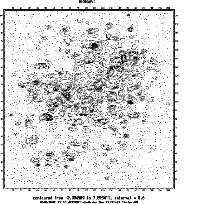
Figure 2: (a). Optical layout of the speckle interferometer, (b). Speckles of the close binary star HR4689 obtained with the new speckle interferometer at VBT. The numbers on the axes denote pixel numbers with each pixel being equal to 0.015 arcsec.

This interferometer is built with extreme care so to avoid flexure problems which might affect high precision measurements of close binary star systems etc., in an unfavourable manner. The design analysis has been carried out with the modern finite element method [41] and computer aided machines were used in manufacturing to get dimensional and geometrical accuracies. The method requires the structure to be subdivided into a number of basic elements like beams, quadrilateral and solid prismatic elements etc. A complete structure is built up by the connection of such finite elements to one another at a definite number of boundary points called nodes and then inputting appropriate boundary constraints, material properties and external forces. The relationship between the required deformations of the structure and the known external forces is $[K]\{{\bf d}\}={\{\bf F}\}$, where, $[K]$ is the stiffness matrix of the structure, $\{{\bf d}\}$ is the unknown displacement vector and $\{{\bf F}\}$ is the known force vector. All the geometry and topology of the structure, material properties and boundary conditions go into computation of $[K]$. The single reason for universal application of finite element method is the ease with which the matrix, $[K]$ is formulated for any given structure.

5.4 Aperture Synthesis :

Two promising methods, viz., (a) speckle masking (see chapter 7.3) technique [42], (b) non-redundant aperture masking technique [6, 7] are based on the principle of phase-closure method. To recover the Fourier phases of the source brightness distribution from the observations, it is necessary to detect fringes on a large baselines, therefore, enables one to reconstruct images. The concept of using three antennae arranged in a triangle was first introduced in radio astronomy [43] in late fifties. Closure-phases are insensitive to the atmospherically induced random phase errors, as well as to the permanent phase errors introduced by the telescope aberrations in optics. Since any linear phase term in the object cancels out [44], this method is insensitive to the position of the object but sensitive to any object phase non-linearity.

The measurements of the closure-phases was first obtained at high light level with three-hole aperture mask placed in the pupil plane of the telescope [5]. Interference patterns of the star were recorded using CCD as sensor. We had conducted similar experiment around the same time by placing an aperture mask of 3-holes, 10cm in diameter, arranged in a triangle, over 1 meter telescope at VBO, Kavalur and tried to record the interference pattern with our earlier version of the interferometer [21]. In this experiment, we used a 16mm movie camera as detector. The advantage of placing aperture mask over the telescope, in lieu of pupil mask is to avoid additional optics. But a curious modulation of intensity in the fringe pattern was noticed, therefore, unable to proceed further. The modulation could result from a time-independent aberration in the optical system of the telescope [21]. However, we performed the similar experiment in the laboratory, using the aperture mask of 3-holes, placed in front of a simulated telescope and were able to record the interference patterns [30].

The aperture synthesis imaging technique with telescope involves observing an object through a masked aperture of several holes and recording the interference patterns in a series of short-exposure. The patterns contain information about structure of the object at the spatial frequencies from which an image of the same can be reconstructed by measuring the visibility amplitudes and closure phases. This method produces images of high dynamic range, but restricts to bright objects.

Several groups have obtained the fringe patterns using both non-redundant and partially redundant aperture mask of N-holes at large or moderate telescope [8-15]. In the laboratory, the shapes of fringe pattern of N-hole apertures were also studied by us by introducing the various aperture masks arranged in both non-redundant and partially redundantly [22, 29]. A few instruments developed for the pupil plane aperture mask are described below.

(i) The instrument developed for the Hale 5 meter telescope [11] used f/2.8 ($\phi$ 85mm) Nikkon camera lens to collimate f/3.3 primary beam of the telescope. The lens formed an image of the primary mirror at a distance of about 85 mm where a mask was placed on a stepper-motor-driven rotary stage controlled by a PC. Another identical lens forms a second focus (scale is 12 arcsec/mm). This image was expanded by microscope objective (X80), enabling to sample 0.15 arcsec/mm on the detector. A narrow band interference filter (6300$\AA$, FWHM 30$\AA$) was placed between the microscope objective and the detector. The resistive anode position sensing photon counting detector [45] was used to record the interference patterns. They were successful in producing optical aperture synthesis maps of two binary stars $\beta-CoronaBorealis$ and $\sigma-Hercules$.

(ii) University of Sydney [12] had developed a masked aperture-plane interference telescope (MAPPIT) for the 3.9 meter Anglo-Australian telescope to investigate interferometry with non-redundant masks. A field lens re-images the telescope pupil down to diameter of 25 mm and the aperture mask is placed where the pupil image is formed. Dove prism is used to rotate the field, allowing coverage of all position angles on the sky. Dispersed fringes are produced using a combination of image and pupil plane imaging. The camera lens and microscope objective produce an image of a star in one direction. In the orthogonal direction, the detector receives the dispersed pupil image. The mask holes play the role of the spectrograph slit. A cylindrical lens is used as the spectrograph’s camera lens. Image photon counting system is used in this experiment to record the dispersed fringe pattern. This instrument is used at coudé focus of 3.9 meter Anglo-Australian telescope. They were able to resolve several close binaries, as well as to measure angular diameters of cool stars [13, 14].

Recently, Bedding [15] of the said University has developed another version of this technique, called multiplexed one-dimensional speckle [MODS], by replacing holes in the aperture mask with a slits. Using a cylindrical lens that creates a continuous series of one-dimensional interferograms, interferograms from many arrays can be recorded side-by-side on a 2-dimensional detector. A narrow band filter is used in place of dispersing prism. The mask containing slit is placed in the collimating beam. The optics in the interference direction form a image plane interferometer and in the orthogonal direction, the cylindrical lens produces a pupil image. Measurements at different position angles can be made by rotating this lens. Two-dimensional image reconstruction can be made from the series of one-dimensional interferograms [46]. Since the same number of photons will be collected in this technique as the conventional speckle interferometer, the limiting magnitude would not change [15].

5.5 Detector :

The speckle interferometer requires snap shots of very high time resolution of the order of (a) frame integration of 50 Hz [47], (b) photon recording rates of a few MHz [48]. We have been using an uncooled ICCD as sensor to record speckle-grams of the objects. It gives video signal as output. The images were recorded at an exposure 20 msec using a frame grabber card DT-2861 manufactured by Data Translation^TM. Each frame consists of odd and even field. But the coherence time of the atmosphere is a highly variable parameter [49], it is desirable to observe speckles with a photon counting system. In the following, we shall describe the salient features of precision analogue photon address (PAPA) detector.

The PAPA is a 2-d photon counting camera [48]. Individual photons hitting the photocathode of a high gain image intensifier produce a spot of light from a phosphor screen on the output side of the intensifier. An image of the phosphor screen is sent through optics to 19 photo-multiplier tubes (PMT), 18 of which have their active area covered by one of 9 different grey scale masks. The 19th tube acts as an event strobe, registering a digital pulse if the spot on the phosphor is detected by the instrument. 9 tubes are used to obtain positional information for an event in one direction, while the other 9 are used for positional information in the orthogonal direction. If the phosphor hit in a region where it is not covered by the mask, an event is registered by the phototube. By taking the information from each phototube for each event, these are recorded as a list of photon addresses and arrival times in a binary format.

6. Data Processing

Stellar speckle interferometry consists of taking many short integration images of an object. The frame image is the convolution of the instantaneous PSF of telescope$-$atmosphere $S(\bf x)$ with the actual object irradiance distribution $O(\bf x)$. The intensity distribution $I(\bf x)$ of the speckle interferograms, in the case of quasi-monochromatic incoherent source can be described by the following space-invariant imaging equations.

$${I(\bf x)={O(\bf x)\ast S(\bf x)}}$$ (31)

In the Fourier domain, convolution becomes an ordinary product so that,

$${\widehat{I}(\bf u)={\widehat{O}(\bf u)\cdot\widehat{S}(\bf u)}}$$ (32)

The ensemble averaged power spectrum is given by,

$${<\mid\widehat{I}(\bf u)\mid^{2}>={\mid\widehat{O}(\bf u)\mid^{2}\cdot<\mid\widehat{S}(\bf u)\mid^{2}>}}$$ (33)

Since $\mid\widehat{S}(\bf u)\mid^{2}$ is a random function in which the detail is continuously changing, the ensemble average of this term becomes smoother. The smooth function can be performed on a point source yields $<\mid\widehat{S}(\bf u)\mid^{2}>$. The object autocorrelation can be obtained by inverse Fourier transform. Figure 3 depicts the auto-correlation of a binary star HR5747. The specklegrams of this star were obtained at the Cassegrain focus of the 2.34m VBT using speckle interferometer [21] on 16/17th March 1990. The uncooled ICCD was used as sensor to record the specklegrams; each pixel of this ICCD was sampled to 0.026 arcsec.

Figure 3: Auto-correlation of a binary star HR5747. The speckles were recorded with earlier version of the speckle interferometer [21, 24] on 16/17th March 1990. The numbers on the axes denote pixel numbers with each pixel being equal to 0.026 arcsec.

7. Image Processing

Several methods have been developed to produce a map of the phase portion of the diffraction limited object Fourier transform. In the following we shall discuss some of the techniques.

7.1 Speckle Holography :

I. In speckle holographic technique [50] complete image reconstruction becomes possible when a reference print source is available in the field of view (within isoplanatic patch $<$ 7 arcsec).

Let us represent the point source by a Dirac impulse $A\delta(\bf x)$ at the origin and let $O_{1}(\bf x)$ be a nearby object to be reconstructed. The irradiance distribution in the field of view is

$$O(\bf x)=A\delta(\bf x)+O_{1}(\bf x)$$ (34)

A regular speckle interferometric measurement will give the squared modulus of its Fourier transform $\widehat{O}({\bf u})$

$$\mid\widehat{O}(\bf u)\mid^{2}=\mid A+\widehat{O}_{1}(\bf u)\mid^{2}$$

$$=A^{2}+A\widehat{O}_{1}(\bf u)+A\widehat{O}_{1}^{*}(\bf u)+\widehat{O}_{1}(\bf u)\widehat{O}_{1}^{*}(\bf u)$$ (35)

The inverse Fourier transform gives the autocorrelation $C_{o}(\bf x)$ of the field of view

$$C_{o}{(\bf x)}=A^{2}\delta{(\bf x)}+AO_{1}{(\bf+x)}+AO_{1}{(\bf-x)}+C_{o1}{(\bf x)}$$ (36)

where $C_{o1}{(\bf x)}$ is the autocorrelation of the object.

The first and the last term in equation (36) are centered at the origin. If the object is far enough from the reference source, $O(\bf x)$ its mirror image $O{(\bf-x)}$ is therefore, recovered apart from a 180^∘ rotation ambiguity.

II. The alternate idea is to calculate the average cross spectrum between the objects and the reference. Let $O_{1}{(\bf x)}$ and $O_{2}{(\bf x)}$ be respectively the object and reference brightness distributions and $I_{1}{(\bf x)}$ and $I_{2}{(\bf x)}$ their associated instantaneous image intensity distributions. The relation between the objects and the images in the Fourier space becomes

$$\widehat{I}_{1}(\bf u)=\widehat{O}_{1}(\bf u)\cdot\widehat{S}(\bf u)$$ (37)

$$\widehat{I}_{2}(\bf u)=\widehat{O}_{2}(\bf u)\cdot\widehat{S}(\bf u)$$ (38)

where, $\widehat{S}{(\bf u)}$ is the impulse response of the telescope and the atmosphere.

The average cross-spectrum between the object and the reference

$$<\widehat{I}_{1}{(\bf u)}\widehat{I}_{2}^{*}{(\bf u)}>=\widehat{O}_{1}{(\bf u)}\widehat{O}_{2}^{*}{(\bf u)}\cdot<\mid\widehat{S}{(\bf u)}\mid^{2}>_{M}$$ (39)

The equation (39) shows that as the speckle holography transfer function $<\mid\widehat{S}{(\bf u)}\mid^{2}>$ is real, the method is insensitive to aberrations and the phase of the cross spectrum expected value coincides with the phase difference between the object and the reference.

7.2 Knox-Thomson Technique (KT) :

The method [51] involves in interfering $I({\bf u})$ with itself after translating by a small shift vector ${\bf\Delta u}$. The KT correlation may be defined in Fourier space as products of $\widehat{I}({\bf u})$.

$$\widehat{I}({\bf u},{\bf\Delta u})=<\widehat{I}{(\bf u)}\widehat{I}^{*}({\bf u}+{\bf\Delta u})>$$ (40)

This gives us the product,

$$<\widehat{I}{(\bf u)}\widehat{I}^{*}({\bf u}+{\bf\Delta u})>=\widehat{O}({\bf u})\widehat{O}^{*}({\bf u}+{\bf\Delta u})\cdot<\widehat{S}({\bf u})\widehat{S}^{*}({\bf u}+{\bf\Delta u})>$$ (41)

Introducing the phases explicitly in the form $\widehat{O}=\mid\widehat{O}\mid e^{j\phi_{o}}$ etc. and using ${\bf\Delta\phi}=\phi({\bf u})-\phi({\bf u}_{1}+{\bf\Delta u})$, we have

$$\mid\widehat{I}{(\bf u)}\mid\mid\widehat{I}({\bf u}+{\bf\Delta u})\mid e^{j\phi_{I}}=\mid\widehat{O}{(\bf u)}\mid\mid\widehat{O}({\bf u}+{\bf\Delta u})\mid e^{j\phi_{O}}\cdot\mid\widehat{S}{(\bf u)}\mid\mid\widehat{S}({\bf u}+{\bf\Delta u})\mid e^{j\phi_{S}}$$ (42)

If this equation is averaged over a large number of frames, the feature $({\bf\Delta\phi_{S}})=0$. When ${\bf\Delta u}$ is small, $\mid\widehat{O}({\bf u}+{\bf\Delta u})\mid\ \approx\ \mid\widehat{O}({\bf u})\mid$ etc. and so

$$<\widehat{I}{(\bf u)}\widehat{I}^{*}({\bf u}+{\bf\Delta u})>=\mid\widehat{O}({\bf u})\mid^{2}e^{j\Delta\phi_{O}}\cdot(a\ smooth\ function)$$ (43)

from which, together with equation (32), ${\bf\Delta\phi_{O}}$ can be determined.

7.3 Speckle Masking or Triple Correlation Technique (TC) :

In case of non-availability of reference point source within iso-planatic patch, the instantaneous PSF can be estimated from the speckle pattern itself. Weigelt [52] suggested to multiply the object speckle pattern $I({\bf x})$ by an appropriately shifted version of this $I({\bf x}+{\bf x}_{1})$. For a binary star, the shift is equal to the angular separation between the stars, masking one of the two component of each double speckle. The result is correlated with $I({\bf x})$. The Fourier transform of the triple correlation is called bispectrum and its ensemble average [42] is given by

$$\widehat{I}({\bf u}_{1},{\bf u}_{2})=<\widehat{I}({\bf u}_{1})\widehat{I}^{*}({\bf u}_{1}+{\bf u}_{2})\widehat{I}({\bf u}_{2})>$$ (44)

where, $\widehat{I}({\bf u}_{1})$, $\widehat{I}({\bf u}_{2})$, $\widehat{I}({\bf u}_{1}+{\bf u}_{2})$, denote the Fourier transforms of $I({\bf x})$.

In the second order moment or in the energy spectrum, phase information is lost, but in the third order moment or in the bispectrum it is preserved. If we put equation (32) into equation (44), it emerges as,

$$\widehat{I}({\bf u}_{1},{\bf u}_{2})=\widehat{O}({\bf u}_{1})\widehat{O}^{*}({\bf u}_{1}+{\bf u}_{2})\widehat{O}({\bf u}_{2})<\widehat{S}({\bf u}_{1})\widehat{S}^{*}({\bf u}_{1}+{\bf u}_{2})\widehat{S}({\bf u}_{2})>$$ (45)

The relationship shows that the image bispectrum is equal to the object bispectrum times a bispectral transfer function. The object bispectrum is given by,

$$\widehat{I}_{o}({\bf u}_{1},{\bf u}_{2})=\widehat{O}({\bf u}_{1})\widehat{O}^{*}({\bf u}_{1}+{\bf u}_{2})\widehat{O}({\bf u}_{2})$$

$$=\frac{<\widehat{I}({\bf u}_{1})\widehat{I}^{*}({\bf u}_{1}+{\bf u}_{2})\widehat{I}({\bf u}_{2})>}{<\widehat{S}({\bf u}_{1})\widehat{S}^{*}({\bf u}_{1}+{\bf u}_{2})\widehat{S}({\bf u}_{2})>}$$ (46)

The modulus $\mid\widehat{O}({\bf u})\mid$ of the object Fourier transform $\widehat{O}({\bf u})$ can be derived from the object bispectrum $\widehat{I}_{o}({\bf u}_{1},{\bf u}_{2})$ [53].

The phase $\phi({\bf u})$ of the object Fourier transform can also be derived from the object bispectrum. Let $\phi_{b}$ be the phase of the object bispectrum and we get,

$$\widehat{O}({\bf u})=\mid\widehat{O}({\bf u})\mid e^{j\phi({\bf u})}$$ (47)

and

$$\widehat{I}_{o}({\bf u}_{1},{\bf u}_{2})=\mid\widehat{I}_{o}({\bf u}_{1},{\bf u}_{2})\mid e^{j\phi_{b}({\bf u}_{1},{\bf u}_{2})}$$ (48)

Equations (47) and (48) may be inserted into equation (42), therefore, yields the relations,

$$\widehat{I}_{o}({\bf u}_{1},{\bf u}_{2})=\mid\widehat{O}({\bf u}_{1})\mid e^{j\phi({\bf u}_{1})}\mid\widehat{O}({\bf u}_{2})\mid e^{j\phi({\bf u}_{2})}\mid\widehat{O}({\bf u}_{1}+{\bf u}_{2})\mid e^{-j\phi({\bf u}_{1}+{\bf u}_{2})}\rightarrow$$ (49)

$$e^{j\phi_{b}({\bf u}_{1},{\bf u}_{2})}=e^{j\phi({\bf u}_{1})}e^{j\phi({\bf u}_{2})}e^{-j\phi({\bf u}_{1}+{\bf u}_{2})}\rightarrow$$ (50)

$$\phi_{b}({\bf u}_{1},{\bf u}_{2})=\phi({\bf u}_{1})+\phi({\bf u}_{2})-\phi({\bf u}_{1}+{\bf u}_{2})\rightarrow$$ (51)

$$\phi({\bf u}_{1}+{\bf u}_{2})=\phi({\bf u})$$

$$=\phi({\bf u}_{1})+\phi({\bf u}_{2})-\phi_{b}({\bf u}_{1},{\bf u}_{2})$$ (52)

Equation (52) is a recursive equation for calculating the phase of the object Fourier transform at coordinate ${\bf u}={\bf u}_{1}+{\bf u}_{2}$ [53]. If the object spectrum at ${\bf u}_{1}$ and ${\bf u}_{2}$ are known, the phase spectrum at $({\bf u}_{1}+{\bf u}_{2})$ can be computed. But the bispectrum phases are of mod $2\pi$, therefore, the reconstruction in equation (48) may lead to $\pi$ phase mismatches between the computed phase-spectrum values along the different paths to the same point in frequency space. The unit amplitude phasor recursive re-constructor are insensitive to the phase ambiguities and the computing argument of the term, $e^{j\phi({\bf u}_{1}+{\bf u}_{2})}$, can be expressed as,

$$e^{j\phi({\bf u}_{1}+{\bf u}_{2})}=e^{j[\phi({\bf u}_{1})+\phi({\bf u}_{2})-\phi_{b}({\bf u}_{1},{\bf u}_{2})]}$$ (53)

The triple correlation algorithm based on this unit amplitude recursive re-constructor method was developed at our institute for processing the stellar objects [33], as well as for the extended object [54].

7.4 Relationships :

From the sections 7.2 and 7.3, we find the relationship among the two widely used algorithms, namely, KT and TC methods [55]. In autocorrelation technique, the major Fourier component of the fringe pattern is averaged as a product with its complex conjugate and so the atmospheric phase contribution is eliminated and the averaged signal is non-zero (see chapter 4). Unfortunately the phase information is not preserved.

The KT is a small modification of the autocorrelation technique In the KT method, approximate phase closure is achieved by two vectors, ${\bf u}$ and ${\bf u}+{\bf\Delta u}$, and assuming that the pupil phase is constant over ${\bf\Delta u}$. The major Fourier component of the fringe pattern is averaged with a component at a frequency displaced by a vector ${\bf\Delta u}$. The vector displacement ${\bf\Delta u}$ should not force the vector difference ${\bf-u-\Delta u}$ outside the spatial frequency bandwidth of the fringe pattern which, in turn, preserves the Fourier phase difference information in the averaged signal. The atmospheric phase effectively forms a closed loop.

In the bispectrum method a third vector, ${\bf\Delta u}$ is added to form phase closure. When $\lambda\Delta u>r_{o}$, the third vector $\bf\Delta u$ is essential. The KT method fails with this arrangement. In this system, the two apertures are extended to three and the $\Delta u>r_{o}/\lambda$. It can be seen that atmospheric phase contribution is not closed. KT is limited to frequency differences $\Delta u<r_{o}/\lambda$. If the bispectrum average is performed, the phase is closed and Fourier phase difference information is preserved. This method can obtain phase information for phase difference $\Delta u>r_{o}/\lambda$.

7.5 Blind Iterative Deconvolution Technique (BID) :

In this technique, the iterative loop is repeated enforcing image-domain and Fourier-domain constraints until two images are found that produce the input image when convolved together [56, 57]. The image-domain constraints of non-negativity is generally used in iterative algorithms associated with optical processing to find effective supports of the object and or PSF from a speckle-gram. The implementation of the BID, used by us is described below.

The algorithm has the degraded image $I({\bf x})$ as the operand. An initial estimate of the PSF, $S({\bf x})$, has to be provided. The degraded image is deconvolved from the guess PSF by Wiener filtering, which is an operation of multiplying a suitable Wiener filter ( constructed from the Fourier transform $\widehat{S}({\bf u})$ of the PSF) with the Fourier transform $\widehat{I}({\bf u})$ of the degraded image. The technique of Wiener filtering damps the high frequencies and minimizes the mean square error between each estimate and the true spectrum. This filtered deconvolution takes the form

$$\widehat{O}({\bf u})=\widehat{I}({\bf u)}{\frac{\widehat{O}_{f}({\bf u})}{\widehat{S}({\bf u})}}$$ (54)

The Wiener filter, $\widehat{O}_{f}({\bf u})$, is given by the following equation:

$${\widehat{O}_{f}({\bf u})={\frac{\widehat{S}({\bf u})\widehat{S}^{*}({\bf u})}{\mid\widehat{S}({\bf u})\mid^{2}+\mid\widehat{N}({\bf u})\mid^{2}}}}$$ (55)

This noise term, $\widehat{N}({\bf u})$, can easily be replaced with a constant estimated as the rms fluctuation of the high frequency region in the spectrum, where the object power is negligible. The Wiener filtering spectrum, $\widehat{O}({\bf u})$, takes the form:

$${\widehat{O}({\bf u})=\widehat{I}({\bf u}){\frac{\widehat{S}^{*}({\bf u})}{\widehat{S}({\bf u})\widehat{S}^{*}({\bf u})+\widehat{N}({\bf u})\widehat{N}^{*}({\bf u})}}}$$ (56)

This result $\widehat{O}(\bf u)$ is transformed to image space, the negatives in the image are set to zero, and the positives outside a prescribed domain (called object support) are set to zero. The average of negative intensities within the support are subtracted from all pixels. The process is repeated until the negative intensities decreases below the noise.

A new estimate of the PSF is next obtained by Wiener filtering the original image $I({\bf x})$ with a filter constructed from the constrained object $O({\bf x})$. This completes one iteration. This entire process is repeated until the derived values of $O({\bf x})$ and $S({\bf x})$ converge to sensible solutions. Before applying this scheme of BID to the real data, we have tested the algorithm with computer simulated convolved functions of binary star and the PSF caused by the atmosphere and the telescope. The reconstruction of the Fourier phase of these are shown in figure 4. The starting guess for the PSF used for this calculation was a Gaussian with random noise. We were able to obtain the output image, as well as the output PSF after 225 iterations.

Figure 4: 2-dimensional maps of the simulated image of (a) binary star, (b) simulated atmospheric PSF, (c) the convolved functions of these two (bpsf), (d) the retrieved image of the binary star, (e) reconstructed atmospheric PSF.

The uniqueness and convergence properties of the deconvolution algorithm are uncertain for the evaluation of the reconstructed images if one uses the BID method directly. We have tested the code [58] and found that it is essential to estimate the input support radius of the object using the auto-correlation technique, which helps in completing the reconstruction satisfactorily after several iterations [32].

8. Astrophysical Programmes

The contribution of single aperture interferometry to several important fields in astrophysics has increased considerably, viz., separation and orientation of close binary stars [32, 59 - 61], shapes of asteroids [62], mapping of the finer features of extended objects [26], sizes of certain types of circumstellar envelopes [63, 64], structures of active galactic nuclei [65, 66], resolving the gravitationally lensed QSO’s [67] etc. We too plan to observe the following interesting objects, if an intensified photon counting detector [48] can be made available.

(i) Studies of binary stars play a fundamental role in measuring stellar masses, providing the benchmark for stellar evolution calculations. A long term benefit of speckle imaging is a better calibration of the main-sequence mass-luminosity relationship. Most measurements have been made at large aperture telescopes by groups in France, Russia, and the United States. Programmes of binary star interferometry are being carried out at telescopes of moderate and small aperture too. But measurements from the southern hemisphere continue to be rare. Many rapidly moving southern binaries are being ignored and a number of discoveries are yet to be confirmed.

(ii) Most of the late-type stars are available in the vicinity of sun. All known stars, within 5 pc radius from the sun are red dwarfs with $m_{v}>$ +15. Due to the intrinsically faint nature of K- and M- dwarfs, their physical properties are not studied extensively. These dwarfs may often be close binaries which can be detected by speckle interferometric technique.

(iii) Another important field of observational astronomy is the studies of the physical processes, viz., temperature, density and velocity of gas in the active region of the active galactic nuclei (AGN). Optical imaging in the light of emission lines on sub-arcsec scales can reveal the structure of the narrow-line gas. The scale of narrow-line regions is well resolved by the diffraction limit of a moderate-sized telescope.

(iv) The spatial distribution of circumstellar matter surrounding objects which eject mass, particularly young compact planetary nebulae can be determined [63, 64].

(v) Capability of resolving the gravitationally lensed QSO’s in the range of 0.2 arcsec. to 0.6 arcsec. will allow the discovery of many more lensing events [67].

9. Epilogue

The understanding of the basic random interference phenomenon $-$ speckle $-$ is of paramount importance to the observational astronomy. In recent years the uses of speckle pattern and a wide variety of applications have been found in many other branches of physics and engineering. Though the statistical properties of speckle pattern is complicated, detailed analysis of this is useful in information processing. Though the stellar speckle interferometry is capable of detecting relatively faint objects ($\sim$ 16th. magnitude), the angular resolution is limited by the diameter of the telescope. Angular resolution can vastly be improved by using long base line interferometry using two or more telescopes.

India has an outstanding group in the field of radio astronomy using long baseline interferometry. From the experience we have gained in developing the field of optical interferometry, we are confident in building a long baseline interferometer in the optical and IR band. Long baseline interferometric observations of the objects [34, 68] would offer the possibilities for direct measurement of all the basic physical parameters for a large number of stars.

References

[1]. H. Fizeau, 1868, C. R. Acad. Sci. Paris, 66, 934.

[2]. A. Labeyrie, 1970, Astron. and Astrophys., 6, 85.

[3]. C. Roddier and F. Roddier, 1988, Proc. NATO-ASI, ’Diffraction Limited Imaging with Very Large Telescopes’, ed. D M Alloin and J M Mariotti, Carg$\grave{e}$se, France, 221.

[4]. R. Petrov, F. Roddier, and C. Aime, 1986, J. Opt. Soc. Am. A., 3, 634.

[5]. J. E. Baldwin, C. A. Haniff, C. D. Mackay, and P. J. Warner, 1986, Nature,

[6]. D. H. Rogstad, 1968, App. Opt. 7, 585.

[7]. W. T. Rhodes and J. W. Goodman, 1973, J. Opt. Soc. Am., 63, 647.

[8]. D. F. Busher, C. A. Haniff, J. E. Baldwin and P. J. Warner, 1990, Mon. Not. Roy. Astro. Soc., 245, 7.

[9]. C. A. Haniff, C. D. Mackay, D. J. Titterington, D. Sivia, J. E. Baldwin and P. J. Warner, 1987, Nature, 328, 694.

[10]. C. A. Haniff, D. F. Busher, J. C. Christou and S. T. Ridgway, 1989, Mon. Not. Roy. Astro. Soc., 241, 51.

[11]. T. Nakajima, S. R. Kulkarni, P. W. Gorham, A. M. Ghez, G. Neugebauer, J. B. Oke, T. A. Prince and A. C. S. Readhead, 1989, A J., 101, 1510.

[12]. T. R. Bedding, J. G. Robertson, R. G. Marson, P. R. Gillingham, R. H. Frater and J. D. O’Sullivan, 1992, Proc. ESO-NOAO conf. ’High Resolution Imaging Interferometry’, ed., J. M. Beckers & F. Merkle, Garching bei München, FRG, 391.

[13]. T. R. Bedding, J. G. Robertson and R. G. Marson, 1994, Astron. Astrophys., 290, 340.

[14]. T. R. Bedding, A. A. Zijlstra, O. Von der Lḧe, J. G. Robertson, R. G. Marson, J. R. Barton and B. S. Carter, 1997, Mon. Not. Roy. Astro. Soc., 286, 957.

[15]. T. R. Bedding, 1999, astro-ph/9901225, Pub. Astron. Soc. Pacific (to appear).

[16]. F. Grieger and G. Weigelt, 1992, Proc. ESO-NOAO conf. ’High Resolution Imaging Interferometry’, ed., J M Beckers and F Merkle, Garching bei M$\ddot{u}$nchen, FRG, 225.

[17]. H. Falcke, K. Davidson, K. H. Hofmann and G. Weigelt, 1996, Astron. Astrophys., 306, L17.

[18]. A. Labeyrie, 1975, Astrophys. J., 196, L71.

[19]. A. Labeyrie, G. Schumacher, M. Dugu$\acute{e}$, C. Thom, P. Bourlon, F. Foy, D. Bonneau, and R. Foy, 1986, Astron. and Astrophys., 162, 359.

[20]. J. E. Baldwin, R. C. Boysen, C. A. Haniff, P. R. Lawson, C. D. Mackay, J. Rogers, D. St-Jacques, P. J. Warner, D. M. A. Wilson, J. S. Young, 1998, Proc. SPIE., on ’Astronomical Interferometry’, 3350, 736. 320, 595.

[21]. S. K. Saha, P. Venkatakrishnan, A. P. Jayarajan and N. Jayavel, 1987, Curr. Sci. 56, 985.

[22]. S. K. Saha, A. P. Jayarajan, K. E. Rangarajan and S. Chatterjee, 1988, Proc. ESO-NOAO conf. ’High Resolution Imaging Interferometry’, ed. F. Merkle, Garching bei M$\ddot{u}$nchen, FRG, 661.

[23]. P. Venkatakrishnan, S. K. Saha and R. K. Shevgaonkar, 1989, Proc., ’Image Processing in Astronomy’, ed. T. Velusamy, 57.

[24]. V. Chinnappan, S. K. Saha and Faseehana, 1991, Kod. Obs. Bull. 11, 87.

[25]. S. K. Saha, B. S. Nagabhushana, A. V. Ananth and P. Venkatakrishnan, 1997, Kod. Obs. Bull., 13, 91.

[26]. S. K. Saha, R. Rajamohan, P. Vivekananda Rao, G. Som Sunder, R. Swaminathan and Lokanadham, B., 1997, Bull. Astron. Soc. Ind., 25, 563.

[27]. S. K. Saha, A. P. Jayarajan, G. Sudheendra, and A. Umesh Chandra, 1997, Bull. Astron. Soc. Ind., 25, 379.

[28]. S. K. Saha, G. Sudheendra, A. Umesh Chandra, and V. Chinnappan, 1998, Experimental Astronomy (to appear).

[29]. S. K. Saha, 1990, VBT News, No., 3, 3.

[30]. S. K. Saha, 1991, IIA Newsletter, 6, 11.

[31]. S. K. Saha, 1991, VBT News, No., 8 & 9, 9.

[32]. S. K. Saha and P. Venkatakrishnan, 1997, Bull. Astron. Soc. Ind., 25, 329.

[33]. S. K. Saha, R. Sridharan and K. Sankarasubramanian, 1999, ’Speckle image reconstruction of Binary Stars’, Presented at XIX ASI meeting held at Bangalore.

[34]. A. Labeyrie, 1988, Proc. NATO-ASI, ’Diffraction Limited Imaging with Very Large Telescopes’, ed. D M Alloin and J M Mariotti, Carg$\grave{e}$se, France, 327.

[35]. M. Born and E. Wolf, 1975, Principles of Optics, Pergamon Press.

[36]. J. A. Anderson, 1920, Astrophys. J., 51, 263.

[37]. A. A. Michelson, 1920, Astrophys. J., 51, 257.

[38]. A. A. Michelson and F. G. Pease, 1921, Astrophys. J., 53, 249.

[39]. D. C. Fried, 1966, J. Opt. Soc. Am., 56, 1972.

[40]. S. K. Saha and V. Chinnappan, 1999, Bull. Astron. Soc. Ind. (to appear).

[41]. O. C. Zienkiewicz, 1967, ’The Finite Element Methods in Structural and Continuum Mechanics’, McGrawhill Publication.

[42]. A. W. Lohmann, G. P. Weigelt and A. Wirnitzer, 1983, Appl. Opt. 22, 4028.

[43]. R. C. Jennison, 1958, Mon. Not. Roy. Astron. Soc., 118, 276.

[44]. S. K. Saha, 1999, ’Emerging Trends of Optical Interferometry in Astronomy’, communicated to Bull. Astron. Soc. India.

[45]. M. Clampin, J. Croker, F. Paresce and M. Rafal, 1988, Rev. Sci. Instru. 59, 1269.

[46]. D. F. Busher and C. A. Haniff, 1993, J. Opt. Soc. Am A., 10, 1882.

[47]. A. Blazit, 1986, Proc., ’Image Detection and Quality’ - SFO, ed., SPIE, 702, 259.

[48]. C. Papaliolios, P. Nisenson and S. Ebstein, 1985, App. Opt. 24, 287.

[49]. R. Foy, 1988, Proc., ’Instrumentation for Ground Based Optical Astronomy - Present and Future’, ed., L. Robinson, Springer Verlag, New York, 345.

[50]. Y. C. Liu, and A. W. Lohmann, 1973, Opt. Comm., 8, 372.

[51]. K. T. Knox, and B. J. Thompson, 1974, Astrophys. J. 193, L45.

[52]. G. Weigelt, 1977, Opt. Communication, 21, 55.

[53]. G. Weigelt, 1988, Proc. NATO-ASI, ’Diffraction Limited Imaging with Very Large Telescopes’, ed. D. M. Alloin and J. M. Mariotti, Carg$\grave{e}$se, France, 191.

[54]. R. Sridharan and P. Venkatakrishnan, 1999, Presented at XIX ASI meeting held at Bangalore.

[55]. G. R. Ayers, M. J. Northcott and J. C. Dainty, 1988, J. Opt. Soc. Am. A, 5, 963.

[56]. G. R. Ayers and J. C. Dainty, 1988, Opt. lett., 13, 457.

[57]. R. H. T. Bates and B. L. K. Davey, 1988, Proc. NATO-ASI, ’Diffraction Limited Imaging with Very Large Telescopes’, ed. D. M. Alloin and J. M. Mariotti, Carg$\grave{e}$se, France, 293.

[58]. P. Nisenson, 1992, Proc. ESO-NOAO conf. ’High Resolution Imaging Interferometry’, ed., J M Beckers and F Merkle, Garching bei M$\ddot{u}$nchen, FRG, 299.

[59]. H. A. McAlister, 1988, Proc. ESO-NOAO conf. ’High Resolution Imaging Interferometry’, ed. F. Merkle, Garching bei M$\ddot{u}$nchen, FRG, 3.

[60]. H. A. McAlister, W. I. Hartkopf, B. D. Mason and M. M. Shara, 1996, Astron. J, 112, 1169.

[61]. W. I., Hartkopf, B. D. Mason, H. A. McAlister, N. H. Turner, B. I. Barry, O. G. Franz and C. M. Prieto, 1996, Astron. J, 111, 936.

[62]. J. Drummond, A. Eckart and E. K. Hege, 1988, Icarus, 73, 1.

[63]. M. J. Barlow, B. L. Morgan, C. Standley, and H. Vine, 1986, Mon. Not. Roy. Astron. Soc., 223, 151.

[64]. P. R. Wood, S. J. Meatheringham, M. A. Dopita and D. M. Morgan, 1987, Astrophys. J., 320, 178.

[65]. V. S. Afanas’jev, I. I. Balega, Y. Y. Balega, V. A. Vasyuk and V. G. Orlov, 1988, Proc. ESO-NOAO conf. ’High Resolution Imaging Interferometry’, ed., F Merkle, Garching bei M$\ddot{u}$nchen, FRG, 127.

[66]. S. Ebstein, N. P. Carleton and C. Papaliolios, 1989, Astrophys. J., 336, 103.

[67]. R. Foy, 1992, Proc. ESO-NOAO conf. ’High Resolution Imaging Interferometry’, ed., J M Beckers and F Merkle, Garching bei M$\ddot{u}$nchen, FRG, 5.

[68]. D. Mourard, I. Bosc, A. Labeyrie, L. Koechlin, and S. Saha, 1989, Nature, 342, 520.

ABOUT THE REVIEWER

Dr. Swapan K. Saha had received his Ph. D (Tech.) from the Institute of Radiophysics and Electronics, Calcutta University in 1983 and is a scientist at the Indian Institute of Astrophysics, Bangalore, India. In mid eighties, his interest had focused on to the ’Optical interferometry in astronomy’ and spent a year at Observatoire de la Cote d’Azur (formerly C E R G A), Caussols, France, to study the high angular features of stars, viz., resolving emission envelope of $\gamma-Cassiopae$, eclipsing binary Algol A - B system etc., using GI2T (Grand Interféromètre à deux télescope), an optical interferometer with a pair of 1.5 metre telescopes on a North-South baseline. He has a strong background in experimental Physics and developed various equipments for carrying out research in different arenas. Among others, the speckle interferometer for the 2.34 meter Vainu Bappu Telescope, Vainu Bappu Observatory, Kavalur, an exceptional one, is used regularly to study the high resolution features of different types of celestial objects, viz., close binary stars, active galactic nuclei, Proto-planetary nebulae etc.; image reconstruction algorithms which preserve the phase in the object Fourier transform, namely, triple correlation technique, blind iterative deconvolution technique are applied to map the atmospherically degraded objects. He is the author of several papers and is a member of International Astronomical Union, as well as a member of Astronomical Society of India.