Hourly Variability in Q0957+561

Abstract

We have continued our effort to re-reduce archival Q0957+561 brightness monitoring data and present results for 1629 $R$-band images using the methods for galaxy subtraction and seeing correction reported previously (Paper I). The new dataset comes from 4 observing runs, several nights apiece, with sampling of typically 5 minutes, which allows the first measurement of the structure function for variations in the $R$-band from timescales of hours to years. Comparison of our reductions to previous reductions of the same data, and to $r$-band photometry produced at Apache Point Observatory (Colley et al. 1999) shows good overall agreement. Two of the data runs, separated by 417 days, permit a sharpened value for the time delay of 417.4 days, valid only if the time delay is close to the now-fashionable 417-day value; our data do not constrain a delay if it is more than three days from this 417-day estimate. Our present results show no unambiguous signature of the daily microlensing, though a suggestive feature is found in the data. Both time delay measurement and microlensing searches suffer from from the lack of sampling at half-day offsets, inevitable at a single observatory, hence the need for round-the-clock monitoring with participation by multiple observatories.

1 Introduction

Previous studies of the Q0957+561 A,B brightness fluctuations have indicated the existence of daily brightness fluctuations. If these are intrinsic to the quasar, then the time delay can be determined to a precision of a fraction of a day; however, if such fluctuations are at least in part due to microlensing, they would probably signal the nature of a baryonic dark matter component.

A recent report by Colley and Schild (ApJ 518, 153, 1999) demonstrated precision aperture photometry close to the photon limit. The procedure subtracts out the lens galaxy’s light according to the galaxy’s profile determined recently from an HST image, and removes cross talk light from the A and B image apertures. We now apply this reduction to 1629 frames collected in 4 runs, with continuous monitoring for 10 hours/night over, typically, 5 nights.

Because previous analysis of these data showed that small brightness fluctuations were observed during these runs, but because the effects of seeing were known to limit conclusions about such low-amplitude fluctuations, we hoped that re-reduction would clarify conclusions about time delay and microlensing. In the first several sections to follow, new results unravel the systematic effects that seeing has on the aperture photometry. Next, the measured brightness fluctuations give a structure function that describes the amplitude of variations observed in this lensed/microlensed system on various timescales. Final sections present time delay calculations and possible microlensing results from two observing runs separated by 417 days.

2 The Photometry

For two decades, RS has monitored Q0957 and amassed a “master dataset” of the variations of images A and B (Schild & Thompson 1995 and earlier references therein). The data presented here come from all-night monitoring in one of two similar observational configurations. About half of the data, as in Paper I, derives from unbinned 1k$\times$1k CCD images with pixel scales of one-third of an arcsecond, exposure times of 450 seconds, read noise of $8e^{-}$, and FWHM seeing of 1.5–2 arcseconds. Some of the data come from otherwise similar circumstances, but derive from a 2k$\times$2k CCD binned down to 1k$\times$1k; here shorter exposure times are used, and the pixel scale is twice as great. Both of these setups typically allow for 5 unsaturated comparison stars in the $R$-band on each data-frame. This paper presents the photometry from more than 1600 such frames.

To reduce 1600 frames, one requires a highly automated photometry reduction code (one free of mouse clicks and manual entry of parameters). In Paper I, we detailed such a method, which is not only automated, but includes two basic improvements upon the basic aperture photometry scheme historically employed to reduce Q0957+561 data images: 1) use of HST imaging to subtract the galaxy, 2) correction for “cross talk” between the narrowly separated ($6.1\arcsec$) A and B images. Typically the galaxy, whose core is inside the B aperture, contributes 17% to the B aperture and 2% to the A aperture. The cross talk contributes typically 2% to each image. One could calibrate those out if the seeing were steady, but poor seeing obviously introduces more cross talk contamination, and has the curious effect of spreading much more galaxy light into the A image. These variable effects confuse the search for both intrinsic QSO variation and microlensing. Worse still, while the seeing introduces a correlation in the A and B photometry (spreading more cross talk light into both images from each other), it also introduces an anti-correlation due to the galaxy, whose light is spread out from the B aperture and into the A aperture. To disentangle these effects, a complete galaxy subtraction and measurement of cross talk is necessary.

Slight modifications to the photometry scheme in Paper I have been implemented, principally for sake of speed and increased automation. As before the astrometry is accomplished via PSF fitting, which requires a model PSF. The model is empirical, built by stacking several standards. The first pass utilizes methods described by Alard & Lupton (1998), but only even terms in the polynomial expansion are used. An explicitly even model PSF for each standard can be fit to the standard itself to determine the astrometry of that standard. Shifting and stacking (by median) all of the standards forms the model PSF. This method has the advantages of being quite fast and of eliminating cosmic rays automatically from the model PSF. Other modifications include increased sensitivity to erratic photometry in the standards (by simply censoring 5-$\sigma$ outliers), and more careful measurement of crosstalk (again by filtering out gross outliers). Each of these methods increase the stability of the photometry appreciably.

3 The Effects of the Lens Galaxy

Fig. 1 shows the contribution of the lens galaxy’s light to the A and B measurement apertures as a function of seeing, as measured from all the image frames of this data set. Plotted is the percentage of the signal in the apertures as a function of FWHM seeing, measured from the stellar images on the data frames. Because seeing effects originate in different levels of the terrestrial atmosphere and do not have a single unique profile, adoption of a simple FWHM parameter is only a first-order statistic and cannot fully describe the variety of seeing profiles supplied by nature.

In the top panel of Fig. 1 the typical percentage contribution to the light of image B is 17.7 percent for average seeing. The average brightness of the B image during this time was 16.51 magnitudes. The observed contribution is equivalent to an 18.39 magnitude source in the measurement aperture. This is in excellent agreement with the R = 18.34 magnitude correction to the lens galaxy magnitude that has been historically adopted throughout the 20-year Q0957 brightness monitoring project (Schild and Weekes, 1984, ApJ 277, 481). The historical correction was made from a compilation of aperture photometry at optical and infrared wavelengths, and the known colors of an elliptical galaxy at moderate redshift. Published data tables of Schild and colleagues usually had a correction for an R = 18.34 magnitude galaxy applied, but no correction for the galaxy contribution to the A aperture and no aperture cross talk corrections.

The bottom panel in Fig. 1 shows the brightness contribution from the lens galaxy to the aperture of the A image. For average seeing, this correction is 3%. Because this contribution originates in the previously unknown outer profile of the lens galaxy, no correction for it has been made in the historical brightness records (where bad seeing images were removed). This has little effect on the historical record, since it just causes a slight reduction in the measured brightness fluctuations of image A, and a slight 3% correction to the inferred A/B continuum brightness ratio.

Best fit parabolic curves have been overplotted on the Fig. 1 data; we give those fits below. With seeing expressed as a FWHM (represented below as $x$) in units of arcseconds, the fitted curves express the percent contribution of the lens galaxy to the R magnitude in a $6\arcsec$ diameter A aperture $\delta R(A)$ and B aperture $\delta R(B)$ as

$$\begin{array}[]{ll}\delta R(A)=[3.154-0.6775x+0.3542x^{2}]\%,\\ \delta R(B)=[18.725-0.5962x]\%.\end{array}$$ (1)

We found that the best fit quadratic term for B was very nearly zero, so we omit that here. These empirical low order fits apply only in the range shown on the plots, and should not be used for seeing with FWHM less than one arcsecond. In such cases, the minimum value shown for the A contamination is probably a quite good approximation, since the curve is obviously flattening by one arcsecond anyway. It seems, however, that the B contamination is still growing as the seeing improves toward one arcsecond, and perhaps one could extrapolate somewhat, but the B contamination would obviously level below some FWHM; hence, correction for the galaxy in the B aperture during very good seeing remains somewhat unresolved.

4 The Aperture Corrections

As the seeing gets worse, relatively more light will spill over from quasar image A into the adjacent B aperture (and vice versa) and cause systematic the cross talk effects noted by Schild and Cholfin, 1986. This effect can be corrected for by measuring the amplitude of the effect in nearby field stars. Insofar as the telescope/camera optics produce no asymmetrical image structure, the effect should be the same for the A and B apertures, as we find here. Thus Fig. 2 shows the aperture correction curve applicable to both apertures, with the amplitude of the crosstalk expressed in percent as a function of seeing FWHM.

The shape and nature of this curve will necessarily depend somewhat on the optics of the telescope/camera and on the properties of the terrestrial atmosphere above Mt Hopkins. We find that a cubic curve represents the crosstalk corrections quite well, and has the following form for $\delta R$ as a function of the seeing FWHM ($x$):

$$\delta R=[0.7087+0.6320x-0.7387x^{2}+0.2788x^{3}]\%$$ (2)

Again, these curves should not be applied for seeing FWHM below one arcsecond, for which the correction evidently flattens out at a value very close to one percent.

Results in this and the previous section show two very different effects of seeing in the two measurement apertures. The crosstalk correction is virtually the same for the two apertures, but the galaxy correction opposes the crosstalk in image B, while adding with the crosstalk for image A. Thus the B image data are substantially more seeing independent than image A data.

Since most of the historical Q0957 data (from the “master dataset” of Schild and Thomson [1995]) were taken with seeing between 1 and 2 arcseconds, the corrections are always less than about a percent. For seeing worse than 2.5 arcseconds, the observations have been heavily censored in the past, which Fig. 2 demonstrates to be important since seeing effects can produce photometric errors of several percent.

5 Results: The Brightness Record

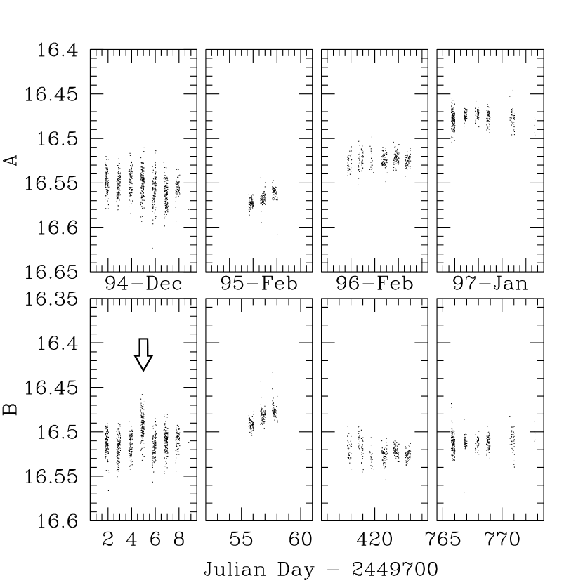
Figure 3: Brightness record after corrections for the lens galaxy and aperture crosstalk. Each data point is for a single image frame, and the “swarms” give an idea of the spread of photometry image to image. Despite the photon noise scatter, variations night-to-night are visible. One particularly interesting feature is in the B data from 1994-December, pointed out by the arrow, where for a single night the B image jumps by 2%. Nightly averages for this data are shown in Fig. 4b) and the hourly binned data for 94-Dec and 96-Feb are shown as Fig. 7)

The final brightness data after corrections for the lens galaxy and aperture cross talk appear in Fig. 3. Plotted points are the result from each data frame, so the amplitude of the “swarm” for each night relates to the accuracy of the photometry. The accuracy is comparable to our results in Paper I, where it was found that the photometry is within 15% of the limit imposed by Poisson statistics. Note that the swarm for the first observing run in Dec. 1994 covering Julian Dates 2449702–08 has a larger amplitude than for later runs; this is because the pixel size was larger by a factor of two on the first observing run, so exposure times are four times shorter and the Poisson noise greater. But although the noise per image frame was larger, there are more of them and the overall precision of the photometry is about the same as for subsequent observing runs.

Correlations in the A and B photometry could arise due to coherent observational errors, such as crosstalk (Schild and Cholfin 1986), though no significant correlation appear (verified by the Pearson’s correlation coefficient applied to raw, galaxy subtracted, and crosstalk corrected photometry). Although it might at first appear that correlated fluctuations were seen in the Feb 1995 run, with both images brightening with time, note that during this time the A image was unusually faint and the B image was unusually bright. So we conclude that by chance, both images were seen brightening at the same time.

These brightness records give unambiguous evidence of daily brightness fluctuations. The best is the record for image B on night 2449704, which we have highlighted with an arrow in Fig. 3 (the same feature is just as obvious in the uncorrected photometry). Here image B increased in brightness by more than 2% from the night before, and returned to its normal level the night after. We conclude that the quasar lens system is capable of producing 2% brightness fluctuations on a time scale of a day. In section 7 below we will compute the structure function for Q0957 brightness fluctuations on long and short time scales.

6 Comparison of Old and New Reductions

The new reductions allow a comparison with the original CCD data record published by Schild and colleagues over the years. Their data are available in tabular form at URL: http://cfa-www.harvard.edu/$\!\sim\!\,$rschild. The data have also been published in Schild & Thomson (1995, and references therein). Here we are concerned with the question of how well the new reductions agree with the original published and tabulated data. Recall that the basic procedure in both the old and new reductions is aperture photometry, and that the new reduction differs primarily in the treatment of subtraction of the lens galaxy G1 and in the correction for aperture crosstalk.

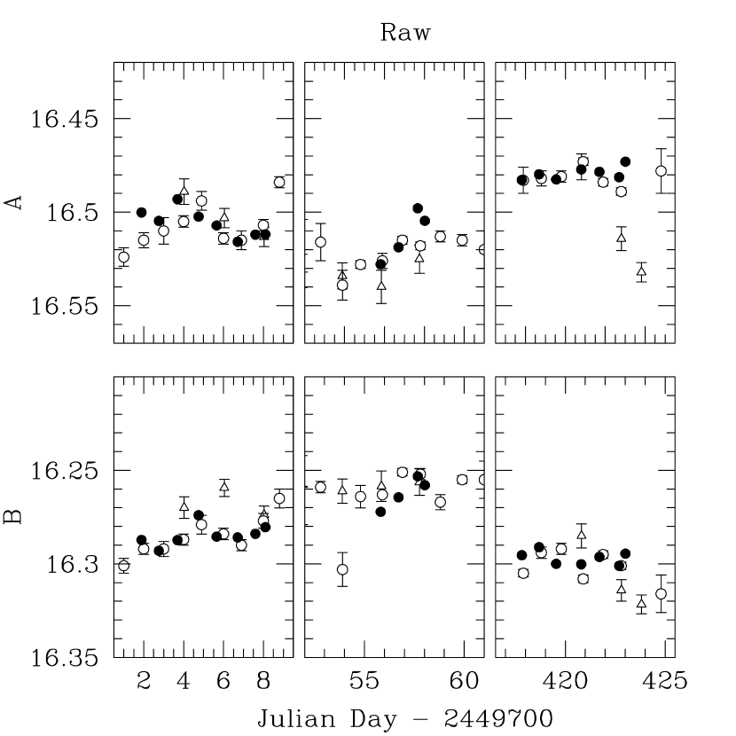
Figure 4: a) Comparison of old and new reductions. Plotted as filled circles are the new nightly brightness averages with no correction for galaxy subtraction or aperture cross talk, to be comparable with the previously published photometry. The errorbars are often smaller than the plot symbols. In open circles, are points from Schild & Thomson (1995); triangles are $r$-band data from Princeton. A single offset of 0.61 magnitudes has been applied to the Princeton photometry, and a single offset of $-0.18$ magnitudes has been applied to the Schild image B photometry, to compensate for his galaxy subtraction. It may be seen that the old Schild reductions using IRAF software produced results very similar to the new reductions.

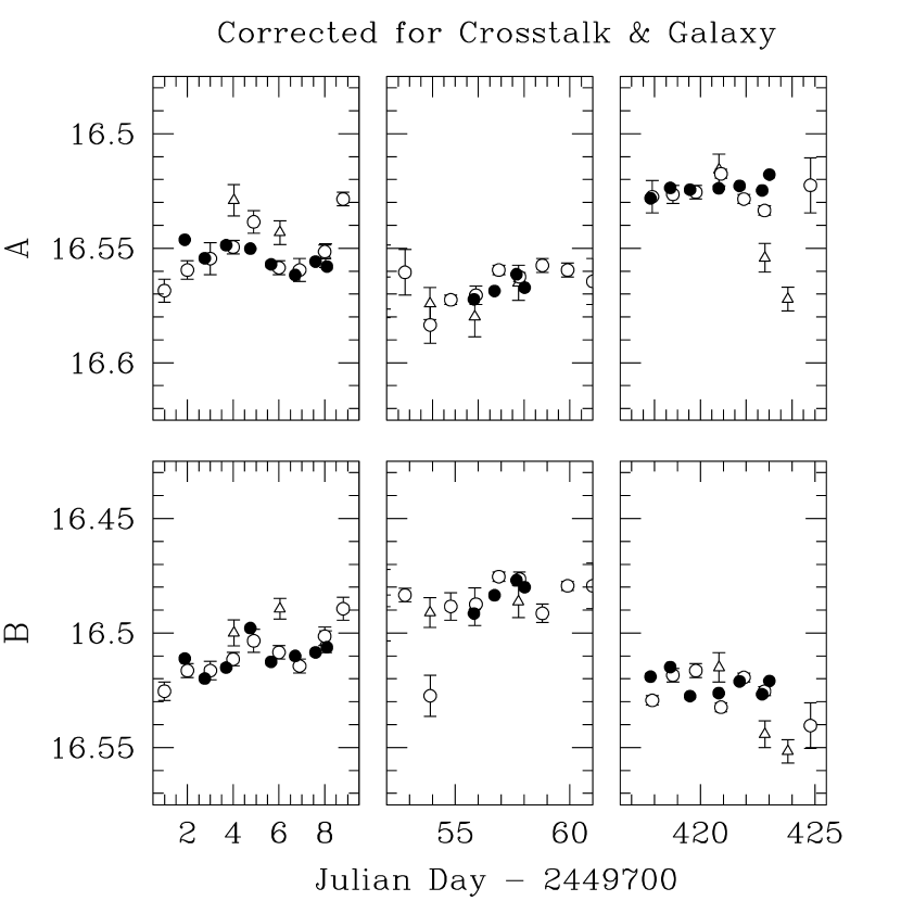
Figure 4: b) As with Fig. 4a), except the filled circles represent photometry which has been corrected for the galaxy and for crosstalk. An arbitrary overall offset has been allowed for A and B, since the photometry from Schild & Thomson, and from Apache Point has not had neither the galaxy subtracted nor crosstalk corrected.

Plotted in Figs. 4a) and b) are the photometry from this work in filled circles. In open circles are plotted the previous reductions of these data from Schild’s master dataset. In open triangles is the $r$-band photometry from Apache Point (Colley et al. 1999). Fig. 4a) shows the comparisons with the raw aperture photometry in this work, while Fig. 4b) gives the comparisons with the corrected photometry.

In Fig. 4a), no correction or shift has been applied to either the old or new photometry for image A. The overall agreement is obviously quite good (almost always within 2%). Meanwhile, for image B, we have simply added back in the galaxy light subtracted in Schild’s master dataset (his 18.34 magnitude galaxy correction), and there is quite good agreement (rarely exceeding more than 1% error). The reason the observation times appear slightly different for these two datasets is that in the Schild dataset, filtering for seeing removed large fractions of data from each run and hence shifted the mean time of observation for each night. If one linearly interpolates the Schild data and compares directly to the photometry of this work, one finds that the image A photometry averages just 3 mmag brighter than Schild’s, with a standard deviation of 8 mmag (statistically consistent with no offset at all). If one does the same for image B, one finds an average discrepancy of 184 mmag with a standard deviation of 6 mmag. This 184 mmag means there is an additional 18.31 magnitude source in our raw B aperture, very close to the 18.34 mag correction Schild made for the lens galaxy.

The [A,B] rms differences between the photometries of only [8,6] mmag show that the nightly averages published by Schild and colleagues are confirmed, since the published errors average about the same amount, which adds credence to many microlensing conclusions reported based upon this data. Note particularly from Fig. 4a) that the discrepancies between the old and new reductions are on a time scale of individual nights, which should not effect the microlensing trends on larger timescales proposed from wavelet analysis by Schild (1999).

Fig. 4b) gives the same data from Schild, but plots our corrected photometry. In previous sections, we discussed the contributions of the galaxy and cross talk during typical seeing. For aperture A the lens galaxy has contributes approximately 3% during typical seeing, while the cross talk between apertures contributes another 1.2%. Our corrected photometry is accordingly 44 mmag fainter than the Schild photometry with an rms of 7 mmag (a slight improvement over the comparison with raw photometry). The image B photometry shows a 40 mmag deficit to the Schild photometry with an rms of 5 mmag (also a slight improvement over the raw photometry). The improvement in rms is perhaps expected, because of the filtering for good seeing done by Schild.

Schild and Thomson (1995) report an internal photometric error of 10 and 12 mmag for A and B respectively during this epoch. Therefore, the agreement of the Schild photometry and current photometry at the 5 mmag level, is about as good as one could expect. It is perhaps noteworthy that the agreement exists despite completely different software for the aperture photometry (IRAF dophot vs. IDL programming from scratch) and completely different methods for the relative photometry (pencil and calculator vs. Honeycutt [1992] matrix reduction).

Because we expect to continue re-reducing archival data frames with our improved data reductions, it is worthwhile summarizing the differences between the new and old reductions. Relative to the old reductions, the new results for image [A,B] are [44, 40] mmag fainter than the tabulated Schild photometry, primarily because of the new corrections for aperture crosstalk but also partly due to improved knowledge of the effects of the lens galaxy. Thus to correct our old photometry to the new system, one would add [.044, .040] mag to the table entries in the Schild master data set. The true errors of the photometry for the dates we have compared are [7,5] mmag.

For reference, the open triangles in Figs. 4a) and b) give the APO $r$-band photometry where applicable (Colley et al. 1999), with arbitrary offsets. While the gross features of the photometry are reproduced, the agreement is not as good, but this might be expected because 1) $r$ is a different filter, 2) no correction or censoring for seeing effects, and 3) the APO photometry derives from only a handful of frames on a given night (hence the larger errorbars), compared with several tens of frames per night at Mt. Hopkins.

7 The Structure Function for Q0957 Brightness Fluctuations

For many purposes related to the discussion of the Q0957 time delay and interpolation of the data set for missing observations, it is useful to know the structure function for the brightness fluctuations. The structure function, which is the expected variance as a function of temporal separation, can be approximated as a power law $V^{2}=10^{a}\cdot\tau^{b}$. For our corrected photometry, we find $a=-4.5;b=0.54$, in rough agreement with values found by Colley et al. (1999) for $r$-band photometry of $a=-4.1;b=0.47$, and by PRH for $R$-band photometry of $a_{A}\approx-0.34;b_{A}\approx 0.54$ and $a_{B}\approx-0.22;b_{B}\approx 0.68$ for the A and B images respectively. The difference in the A and B power laws in PRH shows that measurement of the structure function is perhaps not the most stable process (even perhaps not the best way to describe QSO variation), and suggests that we should not be troubled by the smallish discrepancies between each of these estimates. Fortunately, within reason, the details of the structure function have little bearing on the PRH statistic itself.

Fig. 5 contains a plot of the structure function for the fluctuations averaged for images A and B. Note that Schild (1996) has found from wavelet analysis that the A and B images have equal brightness fluctuations on time scales from days to 2 months, and Pelt et al (1998) have shown that on time scales of decades, the fluctuations are larger in B, presumably because of its larger optical depth to microlensing.

Fig. 5 shows the structure function for time scales of less than a day for the first time. Note that there is no obvious departure from the power law from the smallest to the longest scales. For time scales of a day, the results are consistent with the frequent remark by Schild (1996) that this quasar’s daily brightness fluctuations are typically of order a percent (0.6 percent according to this plot).

8 Time Delay Estimates

Because two of the observing runs, December 1994 and February 1996 were separated by 417 days, the presently favored value of the time delay (Colley et al. 1999, Pelt et al. 1998), it should be possible to determine the gravitational lens time delay to a fraction of a night. We have completed two time delay calculations for the new data. For both of the calculations, to be discussed below, the data have been binned by one hour.

Our first calculation, shown as a dotted line in Fig. 6, is based upon simple linear interpolation of the data and is equivalent to the calculation by Kundić et al (1997, ApJ 482, 75), in which errors and values are linearly interpolated between the nearest points, and a simple $\chi^{2}$ statistic is computed. This autocorrelation calculation produces a network of minima separated by 1.0 days, with the deepest minimum occurring for 417.3 days.

A time delay calculation using the Press, Rybicki, and Hewitt (1992) calculation is shown as the solid line in Fig. 6. This calculation uses the Fig. 5 structure function to estimate the permitted range of brightness values in place of linear interpolation. It also shows a network of minima separated by 1.0 days with the deepest minimum at 417.5 days.

These minima at $n+1/2$ days can be understood easily in terms of the statistics used to compute the best-fit time delay, both of which prefer not to overlap data. The linear method prefers no overlap for a simple reason. Because the data are binned by one hour, the actual number of data in the first and last bin varies according to chance. When a small number of data occurs in those bins, the errorbars are, of course, larger by root-n, than those of typical bins. Hence the linearly interpolated errors are larger by the same factor and are thus far more tolerant in the no-overlap regions. The unusually large errorbars at the end points also explains why the absolute $\chi^{2}$ minimum for the linear method is less than one.

The PRH method prefers no overlap for a different reason, but with similar results. The PRH method, of course, finds that the structure of variations of A and B independently match the structure function (Fig. 5) measured from the A and B variations. It tries to keep A and B independent rather than fighting to find the correct overlap. This propensity to find the gaps was recognized as a possible weakness of PRH by its authors in the original paper.

While both of these methods have proven excellent for determining the time delay for well-sampled data on different timescales (Colley et al. 1999), both show weakness for intermittently sampled data, inevitable at a single observatory at mid latitudes. Because of this complication we conclude that our program of intensive monitoring over many nights separated by the time delay does not allow us to sharpen the time delay significantly, and we do not claim that our overall best fit value 417.4 days is an improvement over other recent determinations. This problem motivates the need for round-the-clock monitoring of the QSO.

9 Agreement of the Time Shifted Brightness Curves

Fig. 7 contains the December 1994 A brightness record (filled circles) and the shifted B brightness record (open circles). At bottom the image B photometry has been shifted by the best-fit time delay from the linear interpolation $\chi^{2}$ method; at top the PRH fit is shown. We show both, because of the qualitatively different appearance of the fits, and because we have no predisposition to favor either method particularly. For reasons discussed in the previous section, we might be inclined to place more faith in the PRH method for producing the best overall fit, because it is less subject to the edge effects due to binning.

In both panels of Fig. 7, there does seem to be a qualitative agreement between the behavior in A and B. Particularly, there seems to be a coherent wavy behavior in both A and B. Some encouragement that the signal is real lies in the fact that night to night neither A nor B shows systematic behavior which is obviously spurious. Namely, neither A nor B is always increasing, decreasing or inflecting in the same way on each night. Such behavior would lead to suspicion that the waviness was an observational artifact. Without “filling in the gaps,” however, the actual validity of these fits is moot, and we are left with only one certainty, that the QSO often varies by about a percent within a given night. This variation means that with round-the-clock observations, highly precise measurement of the time-delay would be possible, and any daily microlensing residing in the signal should become apparent.

Looking at Fig. 7, it is hard to find any definitive microlensing signal, but most suggestive is the apparent gap at JD 2449705.8. While the rest of the curve (in the top panel) seems to obey a coherent pattern, this last interface looks slightly off. This is hardly irrefutable evidence for microlensing, but again, with round-the-clock monitoring, we would be able to be much more definitive if such an event arose. Furthermore, a null result would be of some interest: quasar microlensing searches for the missing mass have been producing exclusion diagrams for possible MACHO masses (Schmidt and Wambsganss 1998, Refsdal et al 1999). The intermittency of microlensing and clumping of caustics (Wambsganss, Witt, and Schneider 1992) are complications, however, and a detection such as the Dec 1994–March 1996 event (Schild and Gibson 1999) is challenging, not so much to observe but to confirm, because of the low amplitudes of the events.

10 Summary and Conclusions

Using improved photometric methods as described in Paper I, we have begun our program of re-reduction of archival Q0957 CCD images acquired over the last 20 years. We report herein results for 4 data runs when the quasar was continuously observed with a 1.2m telescope for typically 6 consecutive nights, including observing runs in Dec 1994 and Feb 1996 which are separated by 417, the currently favored time delay between images A and B (Kundić et al. 1997).

For the new data we show how the contribution of the lens galaxy varies with the seeing. During good seeing the lens galaxy contribution to the A aperture is nearly constant at 2.5% and appears to maximize at about 18.5% in the B aperture. As seeing deteriorates beyond $\mbox{FWHM}=2.5\arcsec$, the A aperture contribution increases by 1% while the B aperture contribution decreases by 1%.

For the same data we evaluate the contribution of A-B aperture cross talk and find that significant deterioration occurs in both apertures for seeing with FWHM greater than $1.8\arcsec$. The deviation from average due to this error source reaches 2% during $\mbox{FWHM}=3\arcsec$ seeing. Thus we find that for deteriorating seeing, galaxy contamination adds to aperture crosstalk in aperture A and compensates for half the cross talk in aperture B. These effects can very significantly affect aperture photometry for the system, but historically they have been only qualitatively understood.

For the fully corrected data we present hourly binned brightness curves that show significantly detected variations on time scales of hours. The quasar can produce 2% brightness fluctuations on the time scales of 24 hours, and 1% brightness fluctuations within individual nights of continuous observation.

Comparison of our new photometry with the previous reductions in the master data set (Schild and Thomson 1995, http://cfa-www.harvard.edu/$\!\sim\!\,$rschild) yields excellent agreement. The new raw photometry agrees with the historical data within an rms of about 7 mmag. The new corrected photometry agrees within slightly better rms limits, after an offset of about +42 mmag is applied to the historical photometry.

With two data runs separated by 417 days, the currently favored time delay, one can search for a more precise delay, and for any daily microlensing residual. Two different time delay estimation procedures favor values near half-day values. These estimators, as would most, tend to find gaps where there is no data overlap between the two runs. The best microlensing candidate in these runs is a significant discrepancy on day 2449705.8 (Fig. 7), which is unfortunately straddling a half-day gap. The tendancy for time delay estimators to find the half-day gaps where either A or B could not be observed due to daylight, and the lack of conclusiveness available for microlensing due to such gaps necessitates round-the-clock monitoring of Q0957+561.

Figure 1: Galaxy Contamination as a function of seeing. Plotted is the percentage of light in the A and B apertures due to the lens galaxy. Contamination by the galaxy not only alters the average photometry of the QSO images, but adds a component which is variable as a function of seeing. This variable component has an amplitude of up to 3% from good ($1\arcsec$) to bad ($2.5\arcsec$) seeing, large enough to corrupt searches for few percent brightness variations. As seeing deteriorates, light of the lens galaxy is systematically scattered out of the image B aperture, which contains the galaxy’s nucleus, but scattered into the A aperture. The fitted curves are discussed in section 3.

Figure 2: Aperture crosstalk as a function of seeing. The crosstalk correction for the A and B images on each data frame is determined from synthesized apertures adjacent to 4 standard stars on each data frame, and averaged. The corrections are the same for the A and B apertures indicating that the star images are symmetrical. The fit curve shown is discussed in Section 4.

Figure 5: The structure function for brightness fluctuations observed in the lensed quasar system, as defined in Section 7. This structure function shows that brightness fluctuations are of order a percent for 1-day lags. Of course both microlensing and intrinsic quasar brightness fluctuations contribute to the fluctuation amplitude.

Figure 6: Measurement of Time Delay from the Dec. 1994 image A data and the Feb. 1996 image B data, binned by one hour (see Fig. 7). Plotted are the $\chi^{2}$ figures of merit from two methods, the Press Rybicki & Hewitt (1992) method (solid curve) and a linear interpolation method (dotted curve) introduced by Kundić et al. (1997). The methods show minima at 417.5 and 417.3 days, respectively. However, both methods also show a troubling sequence of minima at offsets of $\sim(n+1/2)\mbox{~{}days};n\in J$. These minima show up where there is no overlap in the data, due to the sun. Obviously full 24-hour coverage would remedy this situation.

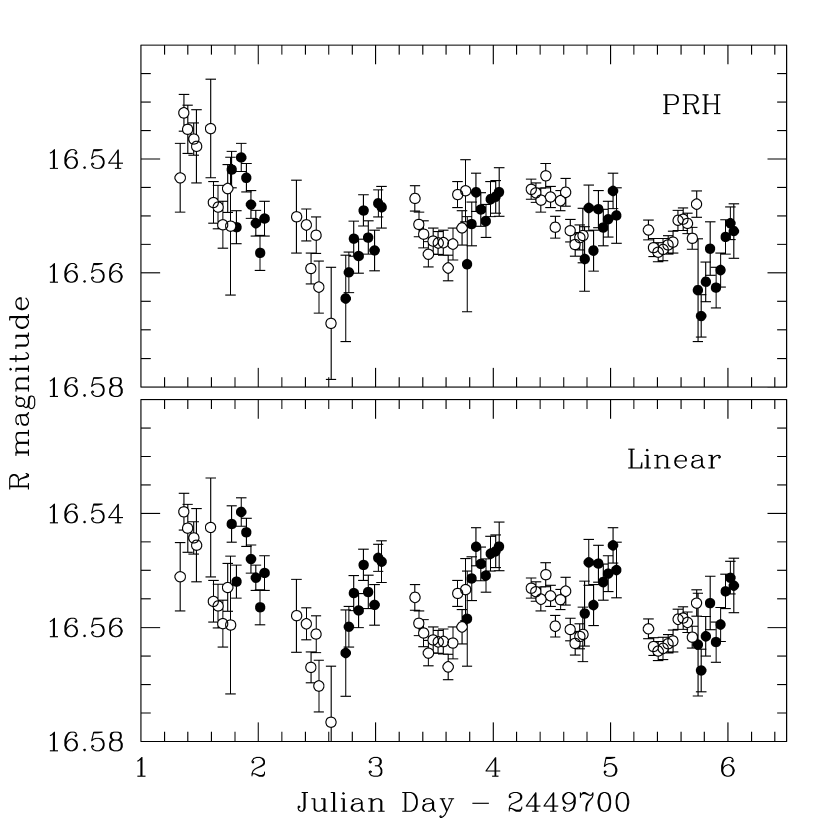
Figure 7: Image A and shifted Image B Data (binned by one hour) in filled and open points respectively. At top, the time delay and offset have been determined by the PRH method, at bottom by a simple linear interpolation scheme (see Fig. 6). Brightness fluctuations of order 1% can be seen during some nights. Such fluctuations should allow determination of the time-delay with a precision of one hour. After such a determination, subtraction of the A light curve from the very precisely shifted B light curve should reveal any short time-scale microlensing. Microlensing on a time scale of a day might be implied by the discontinuity at 2449705 days. Such an event would imply very small MACHO’s ($\sim 10^{-5}M_{\odot}$) in the lens galaxy halo.

References

- (1)
- (2) Alard, C., & Lupton, R. H. 1998, ApJ, 503:325
- (3)
- (4) Colley, W., Turner, E. L., Kundić, T., 1999, in preparation
- (5)
- (6) Colley, W. & Schild, R. 1999, ApJ, 518, 153
- (7)
- (8) Honeycutt, R. K. 1992, PASP, 104, 435
- (9)
- (10) Kundić, T., Turner, E. L., Colley, W. N., et al. 1997, ApJ, 482, 75
- (11)
- (12) Pelt, J., Schild, R., Refsdal, S., & Stabell, R. 1998, A&A, 336, 829
- (13)
- (14) Press, W. H., Rybicki, G. B., & Hewitt, J. N. (PRH) 1992, ApJ, 385, 404
- (15)
- (16) Refsdal, S. et al 1999, Boston Conf. on Gravitational Lensing, ed. T. Brainerd and C. Kochanek, in press
- (17)
- (18) Schild, R. E. 1996, ApJ, 464, 125
- (19)
- (20) Schild, R. E. 1999, ApJ, 514, 598
- (21)
- (22) Schild, R. E., & Cholfin, B. 1986, ApJ, 300, 209
- (23)
- (24) Schild, R. E. and Gibson, C. 1999 astro-ph/9904366
- (25)
- (26) Schild, R. E., & Weekes, T. C. 1984, ApJ, 277, 481
- (27)
- (28) Schild, R. E., & Thomson, D. J. 1995, AJ, 109, 1970
- (29)
- (30) Schmidt, R., & Wambsganss, J. 1998, A&A, 335, 379
- (31)
- (32) Wambsganss, J., Witt, H., & Schneider, P. 1992, A&A, 258, 591
- (33)