Lensing of the CMB: Non Gaussian aspects

Abstract

We study the generation of CMB anisotropies by gravitational lensing on small angular scales. We show these fluctuations are not Gaussian. We prove that the power spectrum of the tail of the CMB anisotropies on small angular scales directly gives the power spectrum of the deflection angle. We show that the generated power on small scales is correlated with the large scale gradient. The cross correlation between large scale gradient and small scale power can be used to test the hypothesis that the extra power is indeed generated by lensing. We compute the three and four point function of the temperature in the small angle limit. We relate the non-Gaussian aspects presented in this paper as well as those in our previous studies of the lensing effects on large scales to the three and four point functions. We interpret the statistics proposed in terms of different configurations of the four point function and show how they relate to the statistic that maximizes the $S/N$.

I Introduction

The anisotropies in the Cosmic Microwave Background (CMB) are thought to contain detailed information about the underlying cosmological model. In conventional models the anisotropies on most angular scales were created at the last scattering surface, at a redshift of $z\sim 1000$. At these early times the evolution of perturbations can be calculated accurately with linear theory. The calculation of theoretical predictions is almost straightforward, thus detailed observations of the microwave sky can, at least in principle, greatly constrain the cosmological model. We expect to be able to measure many of the parameters of the cosmological model with percent accuracy [3].

There are several physical processes that imprint anisotropies on the CMB after decoupling. Some of them will degrade our ability to learn about cosmology, like foreground emission from our galaxy. Others will allow us to constrain processes that happen after decoupling and help us understand the evolution of our universe. For example the reionization of hydrogen by the ultraviolet light from the first generation of objects leaves a distinct mark in the polarization of the CMB [4], Sunyaev-Zeldovich emission from hot gas along the line of sight creates temperature anisotropies and the large scale structure (LSS) of the universe deflects the CMB photons, lensing the anisotropies [5, 6, 7, 8, 11].

When studying the lensing effect produced by the large scale structure of the universe we are trying to detect lensing produced by random mass fluctuations, the LSS, on a random background image, the CMB. The characteristics of the lensing effect depends on the relative size of the coherence lengths of these two random fields. In [7, 8] we studied the limit of a rapidly fluctuating CMB background being lensed by a slowly varying mass distribution. This is the appropriate limit to recover the power spectrum of the projected mass density on scales much larger than the coherence length of the CMB, $\xi\sim 0.15^{o}$. In this paper we study the opposite limit, the generation of power on scales much smaller than $\xi$.

The lensing effect is expected to be the dominant non primordial contribution to the CMB anisotropies on small scales ($l\sim 3000$). It has been shown [9] that an accurate determination of the power generated by lensing can help break some of the parameter degeneracies in the CMB. Interferomentric observations of the anisotropies such as those that will be carried out by CBI [10] are designed to make measurements at these angular scales.

To be able to use the observed power on small scales to break the degeneracies in the parameters one must be sure that one is observing the lensing signal. We will show that the small scale power generated by gravitational lensing has a very definite signature, it is correlated with the large scale gradient. Regions of the sky where the large scale gradient is larger will have more small scale power. The physical effect can be understood easily in the case of a cluster of galaxies lensing a smooth CMB gradient.

We will also compute the general three and four point function of the temperature field induced by lensing and show that both the statistic discussed in this paper and those proposed in [8] are particular subsets of the possible configurations of the four point function. We will construct the statistic that maximizes the signal to noise ratio.

II Generation of power on small scales

The measured temperature field $T({\hbox{\boldmath{$\theta$}}})$ can be expressed in terms of the unlensed CMB field at the last scattering surface $\tilde{T}({\hbox{\boldmath{$\theta$}}})$ and the deflection angle of the CMB photons $\delta{\hbox{\boldmath{$\theta$}}}$,

$$T({\hbox{\boldmath{$\theta$}}}) = \tilde{T}({\hbox{\boldmath{$\theta$}}}+\delta{\hbox{\boldmath{$\theta$}}})$$ (1)

$$\approx \tilde{T}({\hbox{\boldmath{$\theta$}}})+\delta{\hbox{\boldmath{$\theta$}}}\cdot\nabla\tilde{T}({\hbox{\boldmath{$\theta$}}})+{1\over 2}\delta\theta_{i}\delta\theta_{j}\partial_{ij}\tilde{T}({\hbox{\boldmath{$\theta$}}}).$$ (2)

In this paper we are interested in the effect of modes of the deflection angle of spatial wavelength much smaller than that of the unlensed CMB.

A A toy example

To understand the physics we will first consider the lensing induced by a cluster of galaxies. We will discuss a very simplified example in this paper, the reader interested in the detectability of the effect for real cluster should look at reference [14]. In most cases a cluster will subtend a few arcminutes on the sky. Over such a scale the primary anisotropies are expected to have negligible power so we will treat the unlensed temperature field as a pure gradient. Without loss of generality we will take the gradient to be along the $y$ axis with an amplitude $\tilde{T}_{yo}$. The observed temperature becomes,

$$T(\hbox{\boldmath{$\theta$}})=\tilde{T}_{y0}(\theta_{y}+\delta\theta_{y}).$$ (3)

For a spherically symmetric cluster at the origin the deflection is of the form,

$$\delta\hbox{\boldmath{$\theta$}}=-\delta\theta{\hbox{\boldmath{$\theta$}}\over\theta}.$$ (4)

For a singular isothermal sphere $\delta\theta=4\pi(\sigma_{v}/c)^{2}D_{LS}/D_{OS}$, with $\sigma_{v}$ the cluster velocity dispersion, $D_{LS}$ the distance from the lens to the source and $D_{OS}$ that between the observer and the source. In an Einstein DeSitter universe $D_{LS}/D_{OS}\approx 1/\sqrt{1+z_{L}}$, with $z_{L}$ the redshift of the cluster and where we have assumed that $z_{L}$ is much smaller than the redshift of recombination. A singular isothermal profile will be a good approximation for a cluster up to some maximum radius after which the deflection will fall as $1/\theta$. In the central part of the cluster there might be a core. The typical value for $\delta\theta$ is a fraction of an arcminute.

The effect of lensing can be understood by looking at figure 1. We focus on the temperature as a function of $\theta_{y}$ for a fixed $\theta_{x}$. In the absence of lensing we would observe the gradient. On the other hand the cluster will deflect the light rays so that for $\theta_{y}>0$ the rays are coming from a lower value of $\theta_{y}$ in the last scattering surface. If the gradient is positive this implies that for $\theta_{y}>0$ in the presence of the cluster we would observe a lower temperature than what would be observed if the cluster was not there. The opposite is true for $\theta_{y}<0$. Far away from the cluster the lensed temperature should coincide again with the gradient. Thus the cluster creates a wiggle on top of the large scale gradient. This effect is shown in figure 2. The size of this wiggle is $T_{y0}\delta\theta$, thus it is proportional to the size of the gradient and the deflection angle. For a cluster we can use the determined deflection to infer the mass and some information about the cluster profile.

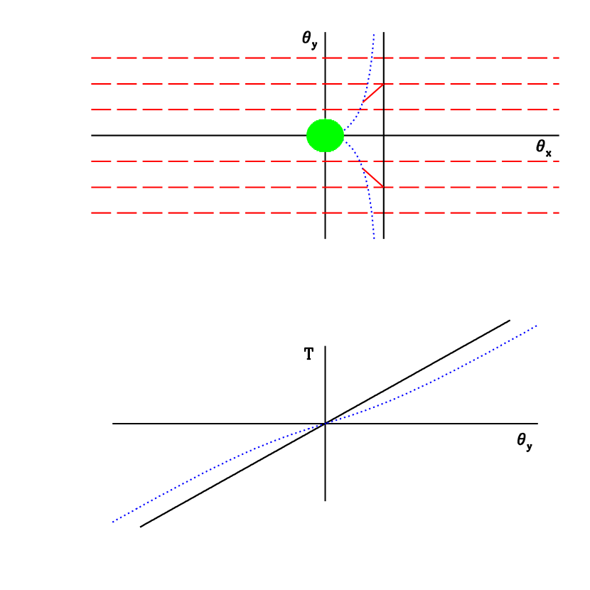
FIG. 1.: In the upper panel we show a cluster lensing a background gradient. The bottom panel shows the temperature measured for a fixed $\theta_{x}$ as a function of $\theta_{y}$ in the presence and absence of the cluster. Points with $\theta_{y}>0$ get deflected to a smaller $\theta_{y}$ in the lens plane and thus for a positive gradient they will have a lower temperature in the lensed example than in the unlensed one. The opposite is true if $\theta_{y}<0$.

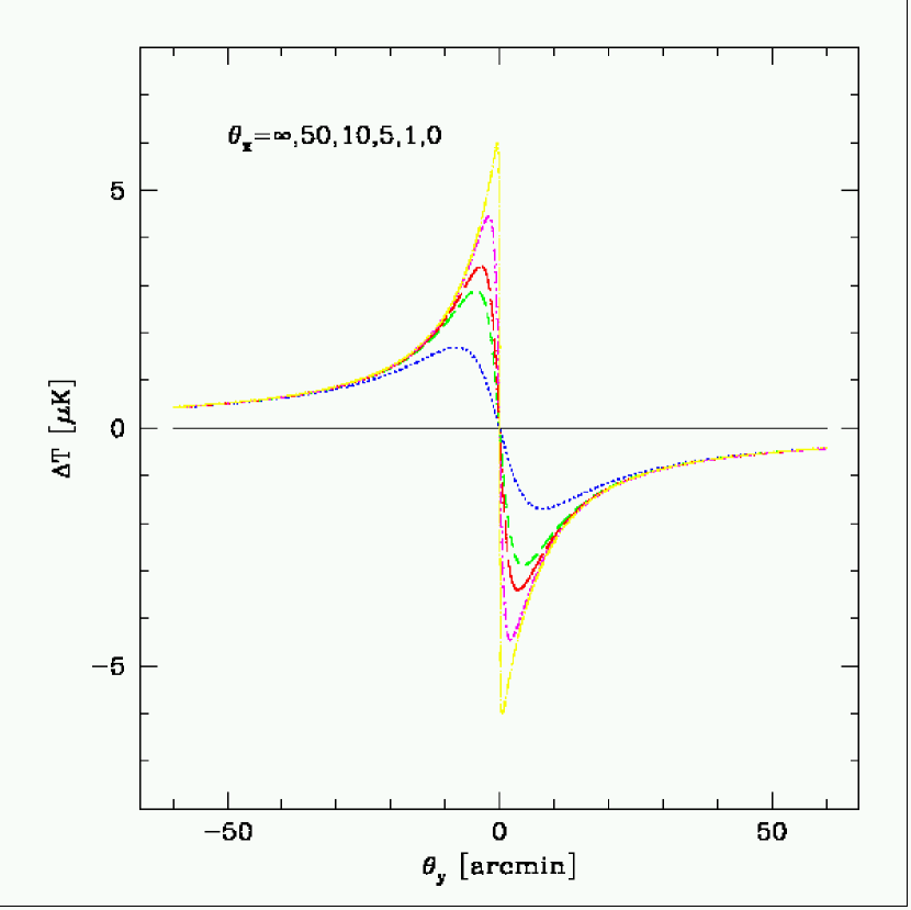
FIG. 2.: Temperature profile of a CMB gradient lensed by a cluster. We took $T_{y0}\delta\theta=13\mu K$. The gradient part has been subtracted out for clarity. The cluster profile was cut-off at $4\ {\rm arcmin}$.

Note that the proposed signal is directly sensitive to the deflection angle and not the shear. This is the only method that has this property. It is usually argued that we can never measure the deflection angle in a lensing system because we do not know the original position of the background image. In this case we avoid this argument because we do know what the background image is, it is a gradient which we can measure on larger scales than the cluster. The other important point is that the effect is proportional to the gradient $T_{y0}$, this is the signature we will use in what follows to identify the lensing effect by large scale structure in the limit we are studying.

B Large scale structure

For simplicity we will work in the small angle approximation so that we can expand the temperature field in Fourier modes instead of spherical harmonics. The Fourier components are defined as,

$$T(\hbox{\boldmath{$l$}}) = \int d^{2}\hbox{\boldmath{$\theta$}}e^{i\hbox{\boldmath{$l$}}\cdot\hbox{\boldmath{$\theta$}}}T(\hbox{\boldmath{$\theta$}})$$ (5)

$$\delta\hbox{\boldmath{$\theta$}}(\hbox{\boldmath{$l$}}) = \int d^{2}\hbox{\boldmath{$\theta$}}e^{i\hbox{\boldmath{$l$}}\cdot\hbox{\boldmath{$\theta$}}}\delta\hbox{\boldmath{$\theta$}}(\hbox{\boldmath{$\theta$}})$$ (6)

We assume both the CMB and the deflection angle are Gaussian random fields characterized by their power spectra,

$$\langle\tilde{T}({\hbox{\boldmath{$l$}}}_{1})\tilde{T}({\hbox{\boldmath{$l$}}}_{2})\rangle = (2\pi)^{2}\delta^{D}({\hbox{\boldmath{$l$}}}_{12})C_{l}^{\tilde{T}\tilde{T}}$$ (8)

$$\langle\delta\hbox{\boldmath{$\theta$}}({\hbox{\boldmath{$l$}}}_{1})\cdot\delta\hbox{\boldmath{$\theta$}}({\hbox{\boldmath{$l$}}}_{2})\rangle = (2\pi)^{2}\delta^{D}({\hbox{\boldmath{$l$}}}_{12})C_{l}^{\delta\delta},$$ (9)

where $\hbox{\boldmath{$l$}}_{12}=\hbox{\boldmath{$l$}}_{1}+\hbox{\boldmath{$l$}}_{2}$, $C_{l}^{\tilde{T}\tilde{T}}$ is the power spectrum of the primary CMB anisotropies and $C_{l}^{\delta\delta}$ is the power spectrum of the deflection angle.

To leading order in the deflection angle the Fourier components of the lensed CMB field are,

$$T({\hbox{\boldmath{$l$}}}) = \tilde{T}({\hbox{\boldmath{$l$}}})+\int{d^{2}{\hbox{\boldmath{$l$}}}^{\prime}\over(2\pi)^{2}}\ \delta{\hbox{\boldmath{$\theta$}}}({\hbox{\boldmath{$l$}}}^{\prime})\cdot\nabla\tilde{T}({\hbox{\boldmath{$l$}}}-{\hbox{\boldmath{$l$}}}^{\prime}).$$ (10)

We want to calculate the power spectrum of the lensed CMB field ($C_{l}^{TT}$) on very small scales, scales much smaller than the coherence length of the unlensed CMB gradient. We start by considering a small patch of the sky of size $L$, with $L$ small enough that the gradient of the unlensed field can be considered constant so that the unlesed CMB map can be approximated linearly. On these scales, the small scale variations of the deflection angle generate additional power in the lensed CMB field. We define $\tilde{T}_{x}(\hbox{\boldmath{$\theta$}})=\tilde{T}_{x0}$ and $\tilde{T}_{y}(\hbox{\boldmath{$\theta$}})=\tilde{T}_{y0}$ so that,

$$T({\hbox{\boldmath{$\theta$}}}) = \tilde{T}_{x0}\ \ [\theta_{x}+\delta\theta_{x}({\hbox{\boldmath{$\theta$}}})]+\tilde{T}_{y0}\ \ [\theta_{y}+\delta\theta_{y}({\hbox{\boldmath{$\theta$}}})].$$ (11)

For the Fourier modes at large $l$ we get,

$$T({\hbox{\boldmath{$l$}}}) = \tilde{T}_{x0}\delta\theta_{x}({\hbox{\boldmath{$l$}}})+\tilde{T}_{y0}\delta\theta_{y}({\hbox{\boldmath{$l$}}}).$$ (12)

Thus the power spectra of the lensed temperature is given by,

$$\langle T({\hbox{\boldmath{$l$}}}_{1})T({\hbox{\boldmath{$l$}}}_{2})\rangle=(2\pi)^{2}\delta^{D}({\hbox{\boldmath{$l$}}}_{12})\sigma_{S}C_{l_{1}}^{\delta\delta}/2,$$ (13)

with $\sigma_{S}=\langle\tilde{T}_{x0}^{2}+\tilde{T}_{y0}^{2}\rangle$. For SCDM $\sigma_{S}\approx 2\times 10^{9}\mu Krad^{-1}\approx 13\mu K{\rm arcmin}^{-1}$. Note that to obtain equation (13) we have replaced $\tilde{T}_{x0}^{2}$ and $\tilde{T}_{y0}^{2}$ by their averages. This implies that we are measuring the power spectrum over a large enough area of the sky that there are many patches over which the gradient is averaged. Equation (13) is a very interesting result on its own, it shows that the power in the tail of the CMB anisotropies directly gives the power spectrum of the deflection angle. This result can also be derived by taking the appropriate limit in the full expression for the lensed CMB spectra as derived for example in [11].

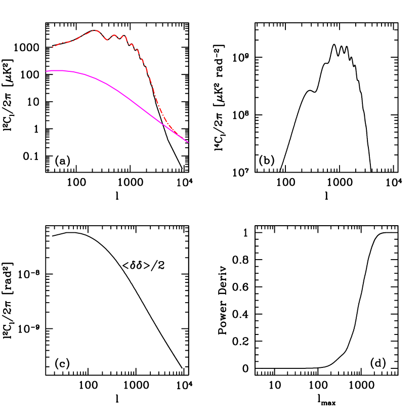
FIG. 3.: The panel (a) shows the lensed and unlensed temperature power spectra together with $\sigma_{S}C_{l}^{\delta\delta}/2$. Panel (b) the power spectra of the derivative of the unlensed CMB field, (c) the spectra of $\delta{\hbox{\boldmath{$\theta$}}}$ and (d) the cumulative power in the CMB derivative.

In figure 3 we show the various power spectra so as to gain some insight on the orders of magnitude. In panel a we show the lensed and unlesed CMB spectra together with $\sigma_{S}C_{l}^{\delta\delta}/2$, the limiting value in the damping tail. Several conditions must be met for equation (13) to be valid. A very important fact is that the power spectra of both the deflection angle and the CMB derivative fall with $l$. This means that when we look at the power generated by lensing in a high $l$ mode of the temperature, it could be dominated by a nearby $l$ of the temperature derivative multiplied by a low $l$ deflection angle mode rather than by the power coming from a small $l$ temperature derivative mode multiplied by a high $l$ deflection mode. Equation (13) is only valid in the latter case. We attain this limit because the power spectra of the deflection angle falls more slowly with $l$ than that of the CMB derivative. The power in the deflection angle falls like a power law (figure 3c) while than in the CMB derivative drops exponentially (figure 3b). As a consequence at a high enough $l$ it is always easier to produce power by multiplying low frequency temperature modes by high frequency deflection modes. At $l>4000$ this effect dominates, at lower $l$ both effect compete. Another condition is that we should apply equation (13) for $l$ values large enough that most of the power in the unlensed derivative (contributing to $\sigma_{S}$) comes from a lower $l$. Figure 3d shows that for SCDM most of the power in the derivative comes from scales $l<2000$.

III Correlation between small and large scales

In the previous section we have shown that the power in the CMB anisotropies at large enough $l$ measures the power spectrum of the deflection angle $\delta\hbox{\boldmath{$\theta$}}$. If we want to use the small scale power to measure the fluctuations in the deflection angle we need a way to determine that the power we observe is indeed produced by lensing and is not at the last scattering surface (ie. it is due to a different underlying primary anisotropies spectrum) or that it is not produced by another secondary effect. To be able to test this we need to consider higher order statistics, we need to go beyond the power spectrum.

The crucial point we are going to use is that the power produced by lensing comes from large scale primary temperature modes promoted to higher $l$ by the small scale deflection of the photons. We will attempt to test the hypothesis that the power we observe is generated by lensing by looking at the correlation between the large scale temperature derivative and the small scale power. If we continue with the simplification that the gradient of the unlensed field is constant, when we high pass filter the temperature map we obtain,

$$T_{H}(\hbox{\boldmath{$\theta$}}) = \int_{l_{h1}}^{l_{h2}}{d^{2}\hbox{\boldmath{$l$}}\over(2\pi)^{2}}e^{-i\hbox{\boldmath{$l$}}\cdot\hbox{\boldmath{$\theta$}}}T(\hbox{\boldmath{$l$}})$$ (14)

$$\approx \tilde{T}_{x}\delta\theta_{x}(\hbox{\boldmath{$\theta$}})+\tilde{T}_{y}\delta\theta_{y}(\hbox{\boldmath{$\theta$}}),$$ (15)

where $l_{h1}$ and $l_{h2}$ define a ring in $l$ space and we have abused notation and called $\delta\theta_{i}(\hbox{\boldmath{$\theta$}})$ the high passed filtered deflection angle. We will study the behavior of the square of $T_{H}$ properly smoothed,

$${\cal H}({\hbox{\boldmath{$\theta$}}}) = \int d^{2}{\hbox{\boldmath{$\theta$}}}^{\prime}W_{H}({\hbox{\boldmath{$\theta$}}}-{\hbox{\boldmath{$\theta$}}}^{\prime})T^{2}_{H}({\hbox{\boldmath{$\theta$}}}^{\prime}).$$ (16)

If we smooth the map over a scale bigger than that of the variations in the deflection angle but over which $\tilde{T}_{x}$ and $\tilde{T}_{y}$ remain constant, we can replace $\delta\theta_{x}^{2}$ and $\delta\theta_{y}^{2}$ by their averages. It follows that the smoothed high passed filtered map is approximately,

$${\cal H}(\hbox{\boldmath{$\theta$}}) \approx {\langle\delta\theta^{2}\rangle\over 2}(\tilde{T}_{x}^{2}+\tilde{T}_{y}^{2})(\hbox{\boldmath{$\theta$}}).$$ (17)

Only the modes with wavevectors $l_{h1}<l<l_{h2}$ contribute to the average $\langle\delta\theta^{2}\rangle$ in equation (17).

We now look at the anisotropies on larger scales by applying a low pass filter to the temperature field,

$$T_{L}(\hbox{\boldmath{$\theta$}}) = \int^{l_{l}}_{0}{d^{2}\hbox{\boldmath{$l$}}\over(2\pi)^{2}}e^{-i\hbox{\boldmath{$l$}}\cdot\hbox{\boldmath{$\theta$}}}T(\hbox{\boldmath{$l$}}).$$ (18)

We compute the square of the gradient,

$${\cal L}(\hbox{\boldmath{$\theta$}}) = ||\nabla T_{L}||^{2}$$ (19)

$$\approx (\tilde{T}_{x}^{2}+\tilde{T}_{y}^{2})(\hbox{\boldmath{$\theta$}}).$$ (20)

Equations (17) and (20) show the maps of ${\cal L}$ and ${\cal H}$ trace each other,

$${\cal H}(\hbox{\boldmath{$\theta$}})\approx{\langle\delta\theta^{2}\rangle\over 2}{\cal L}(\hbox{\boldmath{$\theta$}}).$$ (21)

We have a very simple test to establish that the small scale power is generated by lensing, the small scale power has to be correlated with the large scale derivative. Instead if the small scale power is Gaussian power already present at the last scattering surface, different Fourier modes are uncorrelated. In the Gaussian case if we construct ${\cal L}$ and ${\cal H}$ with different modes ($l_{h1}>l_{l}$) there will be no correlation between the two maps. In practice instead of smoothing the high passed temperature map we work in Fourier space and correlate the low $l$ modes of $T_{H}^{2}(\hbox{\boldmath{$\theta$}})$ with those of the ${\cal L}(\hbox{\boldmath{$\theta$}})$.

Equations (17) and (20) were obtained under simplifying assumptions, more general expressions can also be derived but we only show this limiting case to make the physics more transparent. Comparison with simulations show that this expressions are good approximations in the regime of interest. The procedure to simulate a lensed CMB map was discussed in detail in reference [8]. We generate realizations of CMB and projected mass density $\kappa$ and use a ray tracing technic to produce a lensed CMB map.

We will explain the effect we are studying by first presenting an toy example in 1 dimension. We will consider a 2 dimensional universe so that the last scattering surface becomes a line. In the top panel of figure 4 we show the unlensed CMB field together with the low passed filtered ($l_{l}=2000$) lensed anisotropies. It is clear that both curves trace each other, although they are displaced. This is the consequence of the large scale modes of the deflection angle, but remember we are after the power generated by the small scale modes of $\delta\hbox{\boldmath{$\theta$}}$. In the middle panel we show the high passed ($l>6000$) lensed CMB, the fluctuations in this panel are the result of lensing. The power is not distributed uniformly, the fluctuations are larger where the derivative of the CMB in the top panel is larger, as equation (17) indicates. This is the same physical effect we discussed in the cluster example. On the contrary in regions where the CMB is constant, surface brightness conservation implies that lensing does not create any power. The bottom panel shows the square of the small scale temperature anisotropies and a scaled version of the low $l$ gradient to ease the comparison.

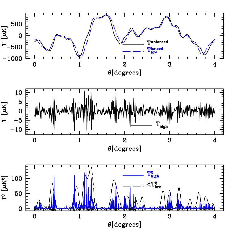
FIG. 4.: Example of the generation of power by gravitational lensing in one dimension. The upper panel shows the unlensed temperature and the result of filtering the lensed $T$. The middle panel shows the high $l$ power generated by lensing. In the bottom we show the square of the small scale power and the square of the large scale gradient (arbitrarily scaled).

We can now look at the results for a 2 dimensional last scattering surface shown in figure 5. The low passed gradient map was constructed using scales $l<2000$ and the high passed temperature was constructed with modes $l>6000$. The upper left panel shows the lensed CMB map while the upper right panel has the high passed filtered field. It is clear that the small scale power in not Gaussian and is higher where the large scale derivative is higher. To make this even more apparent the two bottom panels show the $\cal L$ and $\cal H$ maps, the correlation is excellent.

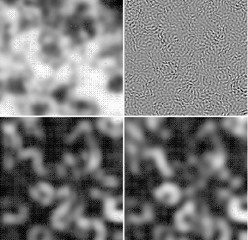
FIG. 5.: The upper panel on the left shows the lensed temperature field. The upper right panel shows the high passed temperature. Bottom left has gradient square and bottom right smoothed square of high passed temperature.

The $\cal L$ and $\cal H$ maps only differ by a factor $\langle\delta\theta^{2}\rangle/2$ (equation 21), so their cross correlation defined as $\langle{\cal H}(\hbox{\boldmath{$l$}}_{1}){\cal L}(\hbox{\boldmath{$l$}}_{2})\rangle=(2\pi)^{2}\delta^{D}(\hbox{\boldmath{$l$}}_{12})C_{l_{1}}^{\cal HL}$, is simply related to the power spectrum of the $\cal L$ map ($C_{l}^{\cal LL}$),

$$C_{l}^{\cal HL} \approx {\langle\delta\theta^{2}\rangle\over 2}C_{l}^{\cal LL}$$ (22)

$$C_{l}^{\cal HH} \approx {\langle\delta\theta^{2}\rangle^{2}\over 4}C_{l}^{\cal LL}$$ (23)

In figure 6a we show the ratio $C_{l}^{\cal HL}/C_{l}^{\cal LL}$ obtained in simulations. We have used $l<2000$ to construct $\cal L$, and several different rings at higher $l$ for $\cal H$. The order of magnitude of the ratio is consistent with equation (23), it remains constant over a wide range of $l$ but starts to fall once we approach $l\sim 2000$. The first relation in equation (23) is really $C_{l}^{\cal HL}=W_{l}{\langle\delta\theta^{2}\rangle}C_{l}^{\cal LL}/2$ where $W_{l}$ is some window function. The origin of the window can be understood as follows: lets call ${\hbox{\boldmath{$l$}}}_{h}$ a high $l$ mode of the deflection and ${\hbox{\boldmath{$l$}}}_{1}$ and ${\hbox{\boldmath{$l$}}}_{2}$ two modes of the derivative. When we compute the gradient square this modes combine to give power at ${\hbox{\boldmath{$l$}}}_{3}={\hbox{\boldmath{$l$}}}_{1}+{\hbox{\boldmath{$l$}}}_{2}$. In the high passed case, we recover this component of the field by looking at the modes with ${\hbox{\boldmath{$l$}}}_{h}+{\hbox{\boldmath{$l$}}}_{1}$ and $-{\hbox{\boldmath{$l$}}}_{h}+{\hbox{\boldmath{$l$}}}_{2}$ so that when we multiply them they give the ${\hbox{\boldmath{$l$}}}_{3}$ variations. As ${\hbox{\boldmath{$l$}}}_{3}$ becomes larger at least one of ${\hbox{\boldmath{$l$}}}_{1}$ or ${\hbox{\boldmath{$l$}}}_{2}$ also become larger and because we are selecting only a ring in $l$ space for the high passed map there are higher chances either ${\hbox{\boldmath{$l$}}}_{h}+{\hbox{\boldmath{$l$}}}_{1}$ or $-{\hbox{\boldmath{$l$}}}_{h}+{\hbox{\boldmath{$l$}}}_{2}$ will fall outside the ring and we cannot reconstruct ${\hbox{\boldmath{$l$}}}_{3}$. So as ${\hbox{\boldmath{$l$}}}_{3}$ gets larger the correlation between the two maps fall. This effect explains the window $W_{l}$ is less important the wider rings for the high passed maps is (compare the high $l$ behavior of the $4000-12000$ and $4000-8000$ rings in figure 6a).

In figure 6b we show the correlation coefficient ${\cal C}_{l}\equiv C_{l}^{\cal HL}/\sqrt{(C_{l}^{\cal HH}C_{l}^{\cal LL})}$. Note that the cross correlation for low $l$ is very high, almost one. This proves our claim that on large scales the $\cal L$ and $\cal H$ maps trace each other almost perfectly. There are several reasons why the two maps do not correlate exactly. First, although most of the power in the derivative of the CMB comes from $l<2000$ there is still about $5\%$ additional power coming from higher $l$. This degrades the cross-correlation because some of the power on the high passed map is coming from these modes of the derivative field. A more extreme case is shown in the figure, where only modes with $l<1000$ were used to construct the $\cal L$ map, the cross-correlation in this case is significantly smaller. The other important effect is that some of the power in the high $l$ map is due to primary anisotropies, these modes are uncorrelated with the low $l$ derivative and thus reduce the cross correlation coefficient. This effect is more important for the $4000-8000$ ring than for the $8000-12000$ so the cross correlation is smaller for the former. The $4000-12000$ rings falls somewhere in the middle of this two cases.

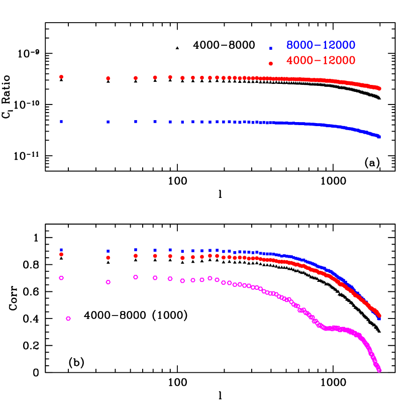
FIG. 6.: Panel (a) shows the ratio $C_{l}^{\cal HL}/C_{l}^{LL}$ for several different rings used to construct $\cal H$. Panel (b) shows the cross correlation coefficient in $l$ space.

We will calculate $C_{l}^{\cal LL}$, which can be done analytically. If we assume that only a Gaussian component is contributing to the low pass filtered field then it is possible to calculate the power spectra of the gradient squared, ${\cal L}=||\nabla T_{L}||^{2}$. The correlation function in real space for two points separated an angle $\theta$ in the $x$ direction gives,

$$\langle{\cal L}(0){\cal L}(\theta)\rangle = \langle{\cal L}^{2}\rangle^{2}+2(C_{xx}^{2}(\theta)+C_{yy}^{2}(\theta)).$$ (24)

We have introduced $C_{xx}(\theta)=\langle T_{x}(0)T_{x}(\theta)\rangle$ and $C_{yy}(\theta)=\langle T_{y}(0)T_{y}(\theta)\rangle$. They are given by,

$$C_{xx}(\theta) \equiv \langle\tilde{T}_{x}(0)\tilde{T}_{x}(\theta)\rangle_{CMB}$$ (25)

$$= (2\pi)^{-2}\int^{l_{l}}d^{2}{\hbox{\boldmath{$l$}}}\ e^{il\cdot\theta\cos\phi_{l}}\ l^{2}C^{\tilde{T}\tilde{T}}_{l}\cos^{2}\phi_{l}$$ (26)

$$= \int_{0}^{l_{l}}{ldl\over 4\pi}\ l^{2}C^{\tilde{T}\tilde{T}}_{l}\left[J_{0}(l\theta)-J_{2}(l\theta)\right]$$ (27)

$$\equiv {1\over 2}[C_{0}(\theta)-C_{2}(\theta)]$$ (28)

$$C_{yy}(\theta) \equiv \langle\tilde{T}_{y}(0)\tilde{T}_{y}(\theta)\rangle_{CMB}$$ (29)

$$= (2\pi)^{-2}\int^{l_{l}}d^{2}{\hbox{\boldmath{$l$}}}\ e^{il\cdot\theta\cos\phi_{l}}\ l^{2}C^{\tilde{T}\tilde{T}}_{l}\sin^{2}\phi_{l}$$ (30)

$$= \int_{0}^{l_{l}}{ldl\over 4\pi}\ l^{2}C^{\tilde{T}\tilde{T}}_{l}\left[J_{0}(l\theta)+J_{2}(l\theta)\right]$$ (31)

$$\equiv {1\over 2}[C_{0}(\theta)+C_{2}(\theta)]$$ (32)

$$C_{xy}(\theta) \equiv \langle\tilde{T}_{x}(0)\tilde{T}_{y}(\theta)\rangle_{CMB}$$ (33)

$$= (2\pi)^{-2}\int^{l_{l}}d^{2}{\hbox{\boldmath{$l$}}}\ e^{il\cdot\theta\cos\phi_{l}}\ l^{2}C^{\tilde{T}\tilde{T}}_{l}\cos\phi_{l}\sin\phi_{l}$$ (34)

$$= 0,$$ (35)

where $C_{0}(\theta)$ and $C_{2}(\theta)$ are defined as the integrals over $l^{3}C_{l}^{\tilde{T}\tilde{T}}dl/2\pi$ weighted with $J_{0}(l\theta)$ and $J_{2}(l\theta)$, respectively.

The constant part in equation (24) only contributes to the $l=0$ mode. The second term is $\sigma_{S}^{2}N^{\cal S\cal S}(\theta)$ in the notation of [8]. The power spectra of the low pass filtered map is that of $\cal S$ in [8], but with only the low $l$ modes included. For $l\neq 0$,

$$C_{l}^{\cal LL} = 2\pi\int\theta d\theta(C_{o}^{2}+C_{2}^{2})J_{0}(l\theta).$$ (36)

This calculation coincides perfectly with the results of simulations. In the presence of detector noise the above expression generalizes to $C_{l}^{\cal LL}\rightarrow C_{l}^{\cal LL}+N_{l}^{\cal LL}$, where $N_{l}^{\cal LL}$ is the detector noise contribution calculated using equations (35) and (36) with the power spectrum of the detector noise.

Let us now consider $C_{l}^{\cal HH}$. If the contribution to the power where Gaussian then the correlation function of $\cal H$ in real space would be,

$$\langle{\cal H}(0){\cal H}(\theta)\rangle = \langle{\cal H}^{2}\rangle^{2}+2C^{2}(\theta)$$ (37)

where,

$$C(\theta) \equiv \langle\tilde{T}_{H}(0)\tilde{T}_{H}(\theta)\rangle_{CMB}$$ (38)

$$= (2\pi)^{-2}\int d^{2}{\hbox{\boldmath{$l$}}}\ e^{il\cdot\theta\cos\phi_{l}}\ C^{\tilde{T}\tilde{T}}_{l}$$ (39)

$$= \int_{l_{h1}}^{l_{h2}}\ {ldl\over 2\pi}C^{\tilde{T}\tilde{T}}_{l}J_{0}(l\theta).$$ (40)

The power spectrum becomes,

$$C_{l}^{\cal HH} = 4\pi\int\theta d\theta C^{2}(\theta)J_{0}(l\theta)$$ (41)

This expression only coincides with the results of simulations when either detector noise or intrinsic CMB anisotropies dominate the power in the $l$ range used to construct $\cal H$, that is if the unlensed power is Gaussian. In the idealized detector noise free examples we have discussed above this corresponds to $l_{h2}<4000$. Fortunately for the power generated by lensing, the power spectra of the $\cal H$ map is a scaled version of the power spectrum of $\cal L$, thus it can be obtained using equations (23) and (38). Again in the presence of noise $C_{l}^{\cal HH}\rightarrow C_{l}^{\cal HH}+N_{l}^{\cal HH}$ with $N_{l}^{\cal HH}$ calculated using equation (41) with the detector noise power spectra.

To assess the signal to noise of our lensing signal we need to calculate the variance in the estimator of $C_{l}^{\cal HL}$,

$$\hat{C}_{l}^{\cal HL}={A_{f}\over(2\pi)^{2}}\int{dA_{l}\over A_{l}}{\cal H}(\hbox{\boldmath{$l$}}){\cal L}(-\hbox{\boldmath{$l$}}),$$ (42)

where the integral is done over a small area in $l$ space of size $A_{l}$ centered around $l$ and $A_{f}=(2\pi)^{2}/\Omega$ is the area of the fundamental cell in $l$ space. We have denoted $\Omega$ the area of sky observed.

If we assume that $\cal L$ and $\cal H$ are Gaussian fields, we can calculate the variance as,

$${\rm Cov}[(\hat{C}^{\cal HL}_{l})^{2}] = {A_{f}\over A}[(C^{\cal HL}_{l})^{2}+C^{\cal HH}_{l}C^{\cal LL}_{l}].$$ (43)

The ratio ${A/A_{f}}$ is the number of available modes one can use to measure the cross correlation. It can be approximated by $A_{l}/A_{f}=f_{sky}(2l+1)$ for a unit width ring. In figure 7 we show the variance in the cross correlation measured in simulations normalized to the Gaussian prediction in equation (43). The agreement is very good implying that we can use the Gaussian formula to compute the variance.

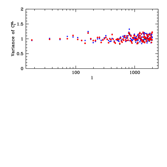
FIG. 7.: Ratio of variance of power spectrum measured in the simulation to the predicted result assuming Gaussian fields.

To compute the total S/N we want to combine the signal in all the $l$ modes of the cross correlation that we can measure. To do this we will compute $\hat{X}=\sum_{l}\alpha_{l}\hat{C}^{\cal HL}_{l}$ choosing $\alpha_{l}$ to maximize S/N$=[\langle\hat{X}\rangle^{2}/{\rm Cov}(\hat{X}^{2})]^{1/2}$. It is straight forward to show that $\alpha_{l}=C^{\cal HL}_{l}/{\rm Cov}[(C^{\cal HL}_{l})^{2}]$, [12]. We then get,

$${S\over N} = \left[\sum_{l<l_{l}}{(C^{\cal HL}_{l})^{2}\over{\rm Cov}[(C^{\cal HL}_{l})^{2}]}\right]^{1/2}$$ (44)

$$= \left[f_{sky}\sum_{l<l_{l}}(2l+1){{\cal C}_{l}^{2}\over((1+N_{l}^{\cal LL}/C_{l}^{\cal LL})(1+N_{l}^{\cal HH}/C_{l}^{\cal HH})+{\cal C}_{l}^{2})}\right]^{1/2}.$$ (45)

We have implicitly assumed rings of unit width.

We want to relate equation (44) to the S/N with which we can measure the small scale power generated by lensing. It is straightforward to show using equations (36), (41) and the fact that ${\cal C}_{l}\sim 1$ that $N_{l}^{\cal HH}/C_{l}^{\cal HH}\approx(w_{T}^{-1}/\bar{C}^{TT})^{2}$, here $\bar{C}^{TT}$ is the averaged power in the band $l_{h1}<l<l_{h2}$ and $w_{T}^{-1}$ is the power spectrum of the detector noise, assumed to be white noise.

We will consider the limit in which $w_{T}^{-1}$ is small enough that $N_{l}^{\cal LL}\ll C_{l}^{\cal LL}$ but is large enough that $N_{l}^{\cal HH}\gg C_{l}^{\cal HH}$. If the noise where even lower then the S/N for detecting the cross correlation will be large S/N$\sim N_{L}^{1/2}$ where $N_{L}$ is the total number of cross correlations that can be measures, $N_{L}\approx f_{sky}l_{l}^{2}$. In the limit we are considering,

$$({S\over N})^{2} = N_{L}{\cal C}_{l}^{2}({\bar{C}_{l}\over w_{T}^{-1}})^{2}$$ (46)

$$= 2{N_{L}\over N_{P}}{\cal C}_{l}^{2}({S\over N})^{2}_{P},$$ (47)

where we have introduced $({S\over N})_{P}^{2}=N_{P}/2(\bar{C}_{l}/w_{T}^{-1})^{2}$, the signal to noise with which we can measure the power in the band $l_{h1}-l_{h2}$. We call $N_{P}$ the number of modes that we can use to estimate the power, which is relate to $N_{L}$ by,

$${N_{L}\over N_{P}}={l_{l}^{2}\over l_{h2}^{2}-l_{h1}^{2}}.$$ (48)

Thus the S/N to measure the cross correlation is comparable although always somewhat smaller than that to detect the power directly. For example if we take $l_{l}=2000$, $l_{h1}=4000$ and $l_{h2}=6000$ then $S/N\approx\sqrt{2/5}{\bar{\cal C}_{l}}(S/N)_{P}$.

IV The three and four point functions in the small angle limit

In this paper and in our previous studies [7, 8, 12] we have investigated several ways of detecting the effect of gravitational lensing on the CMB. As we have explained this amounts to trying to detect the distortions on the random CMB maps created by the random distributions of the dark matter in the universe. In [12] we used the ISW effect as a tracer of the dark matter distribution and combinations of the CMB derivatives to measure the effect of lensing. The cross correlation of these two effects allowed us to gain information about the time evolution of the gravitational potential. Our method combined the information in particular configurations of the three point function of the temperature. Other studies have used other combinations of the bispectrum to detect the signal [6] and also calculated the contributions to the bispectrum coming from other secondary procesess [6, 13].

In [8] we used the power spectrum of quadratic combination of derivatives of the CMB to measure the power spectrum of the projected mass density $\kappa$. This method was valid in the limit in which we wanted to recover the long wavelength modes of $\kappa$ from information in the small scale CMB. This regime is analogous to weak lensing of background galaxies. In essence the different estimates of the power spectrum of $\kappa$ at different scales were obtained by combining different configurations of the four point function of the lensed temperature.

In the present paper we studied other configurations of the four point function to illustrate the nature of the non-Gaussianities induced by lensing on small scales. The non-Gaussian nature of the generated power manifested itself in the correlations between the large scale gradient and the small scale generated power.

In order to have a unified picture of the different statistics we have proposed it is convenient study directly the four point function of the temperature field and a three point function which correlates two temperatures and another field $X$. The field $X$ stands for any field that cross correlates with $\kappa$. In our paper [12] $X=T$ but one can imagine doing this correlation with other tracers of the mass, like the fluctuations of the Far Infrared Background [15].

We define the connected three and four point functions as,

$$\langle X(\hbox{\boldmath{$l$}}_{1})T(\hbox{\boldmath{$l$}}_{2})T(\hbox{\boldmath{$l$}}_{3})\rangle_{c} = (2\pi)^{2}\delta^{D}(\hbox{\boldmath{$l$}}_{123})T_{3}(\hbox{\boldmath{$l$}}_{1},\hbox{\boldmath{$l$}}_{2},\hbox{\boldmath{$l$}}_{3})$$ (49)

$$\langle T({\hbox{\boldmath{$l$}}}_{1})T({\hbox{\boldmath{$l$}}}_{2})T({\hbox{\boldmath{$l$}}}_{3})T({\hbox{\boldmath{$l$}}}_{4})\rangle_{c} = (2\pi)^{2}\delta^{D}({\hbox{\boldmath{$l$}}}_{1234})T_{4}(\hbox{\boldmath{$l$}}_{1},\hbox{\boldmath{$l$}}_{2},\hbox{\boldmath{$l$}}_{3},\hbox{\boldmath{$l$}}_{4}),$$ (50)

Gravitational lensing produces,

$$T_{3}(\hbox{\boldmath{$l$}}_{1},\hbox{\boldmath{$l$}}_{2},\hbox{\boldmath{$l$}}_{3}) = 2C_{l1}^{\kappa X}[C^{\tilde{T}\tilde{T}}_{l2}{\hbox{\boldmath{$l$}}_{2}\cdot\hbox{\boldmath{$l$}}_{1}\over l_{1}^{2}}+C^{\tilde{T}\tilde{T}}_{l3}{\hbox{\boldmath{$l$}}_{3}\cdot\hbox{\boldmath{$l$}}_{1}\over l_{1}^{2}}]$$ (51)

$$T_{4}({\hbox{\boldmath{$l$}}}_{1},{\hbox{\boldmath{$l$}}}_{2},{\hbox{\boldmath{$l$}}}_{3},{\hbox{\boldmath{$l$}}}_{4}) = C^{\tilde{T}\tilde{T}}_{l_{1}}C^{\tilde{T}\tilde{T}}_{l_{2}}\left[{(\hbox{\boldmath{$l$}}_{1}+\hbox{\boldmath{$l$}}_{3})\cdot\hbox{\boldmath{$l$}}_{1}(\hbox{\boldmath{$l$}}_{1}+\hbox{\boldmath{$l$}}_{3})\cdot\hbox{\boldmath{$l$}}_{2}\over||\hbox{\boldmath{$l$}}_{1}+\hbox{\boldmath{$l$}}_{3}||^{2}}C^{\delta\delta}_{l_{13}}+{(\hbox{\boldmath{$l$}}_{1}+\hbox{\boldmath{$l$}}_{4})\cdot\hbox{\boldmath{$l$}}_{1}(\hbox{\boldmath{$l$}}_{1}+\hbox{\boldmath{$l$}}_{4})\cdot\hbox{\boldmath{$l$}}_{2}\over||\hbox{\boldmath{$l$}}_{1}+\hbox{\boldmath{$l$}}_{4}||^{2}}C^{\delta\delta}_{l_{14}}\right]$$ (52)

$$+ {\rm permutations}\ (5\ {\rm terms\ proportional\ to}\ C^{\tilde{T}\tilde{T}}_{l_{1}}C^{\tilde{T}\tilde{T}}_{l_{3}},C^{\tilde{T}\tilde{T}}_{l_{1}}C^{\tilde{T}\tilde{T}}_{l_{4}},C^{\tilde{T}\tilde{T}}_{l_{2}}C^{\tilde{T}\tilde{T}}_{l_{3}},C^{\tilde{T}\tilde{T}}_{l_{2}}C^{\tilde{T}\tilde{T}}_{l_{4}},C^{\tilde{T}\tilde{T}}_{l_{3}}C^{\tilde{T}\tilde{T}}_{l_{4}}).$$ (53)

The unconnected part of the four point function also gets corrections. To make the calculation of these terms fully consistent up to second order in the deflection angle we need to also consider the contributions coming from the second order in the expansion of equation (1). The unconnected terms are not relevant for our study so we will not write them down here.

In our previous papers we introduced three variables $\cal E$, $\cal B$ and $\cal S$. We had defined them in terms of derivatives to the temperature field. Equivalently we can write,

$${\cal S}(\hbox{\boldmath{$l$}}) = \int{d^{2}\hbox{\boldmath{$l$}}_{1}\over(2\pi)^{2}}(\hbox{\boldmath{$l$}}-\hbox{\boldmath{$l$}}_{1})\cdot\hbox{\boldmath{$l$}}_{1}T(\hbox{\boldmath{$l$}}-\hbox{\boldmath{$l$}}_{1})T(\hbox{\boldmath{$l$}}_{1})$$ (54)

$${\cal Q}(\hbox{\boldmath{$l$}}) = \int{d^{2}\hbox{\boldmath{$l$}}_{1}\over(2\pi)^{2}}[(l_{x}-l_{1x})l_{1x}-(l_{y}-l_{1y})l_{1y}]T(\hbox{\boldmath{$l$}}-\hbox{\boldmath{$l$}}_{1})T(\hbox{\boldmath{$l$}}_{1})$$ (55)

$${\cal U}(\hbox{\boldmath{$l$}}) = \int{d^{2}\hbox{\boldmath{$l$}}_{1}\over(2\pi)^{2}}[(l_{x}-l_{1x})l_{1y}+(l_{y}-l_{1y})l_{1x}]T(\hbox{\boldmath{$l$}}-\hbox{\boldmath{$l$}}_{1})T(\hbox{\boldmath{$l$}}_{1})$$ (56)

$${\cal E}(\hbox{\boldmath{$l$}}) = {\cal Q}(\hbox{\boldmath{$l$}})\cos(2\phi_{\hbox{\boldmath{$l$}}})+{\cal U}(\hbox{\boldmath{$l$}})\sin(2\phi_{\hbox{\boldmath{$l$}}})$$ (58)

$${\cal B}(\hbox{\boldmath{$l$}}) = -{\cal Q}(\hbox{\boldmath{$l$}})\sin(2\phi_{\hbox{\boldmath{$l$}}})+{\cal U}(\hbox{\boldmath{$l$}})\cos(2\phi_{\hbox{\boldmath{$l$}}})$$ (60)

When we average over the CMB random field we get,

$$\langle{\cal S}(\hbox{\boldmath{$l$}})\rangle_{CMB} = ((2\pi)^{2}\delta^{D}(\hbox{\boldmath{$l$}})-2\kappa(\hbox{\boldmath{$l$}}))\sigma_{\cal S}$$ (61)

$$\langle{\cal E}(\hbox{\boldmath{$l$}})\rangle_{CMB} = -2\kappa(\hbox{\boldmath{$l$}})\sigma_{\cal S}$$ (62)

$$\langle{\cal B}(\hbox{\boldmath{$l$}})\rangle_{CMB} = 0.$$ (63)

We have introduced $\sigma_{\cal S}=\int ldl/2\pi\ l^{2}C_{l}^{\tilde{T}\tilde{T}}$.

To extract all the information in this three point function se combine all possible configurations with a weight $\beta$ chosen to maximize the signal to noise ratio. We define,

$$\hat{Y} = {A_{f}\over(2\pi)^{2}}\int{d^{2}\hbox{\boldmath{$l$}}_{1}\over A_{l}}{d^{2}\hbox{\boldmath{$l$}}_{2}\over A_{l}}\beta(\hbox{\boldmath{$l$}}_{1},\hbox{\boldmath{$l$}}_{2},\hbox{\boldmath{$l$}}_{3})\ X(\hbox{\boldmath{$l$}}_{1})T(\hbox{\boldmath{$l$}}_{2})T(\hbox{\boldmath{$l$}}_{3}).$$ (64)

For these mildly non-Gaussian maps, the variance can be calculated by only taking the Gaussian part of the temperature, so that

$${\rm Var}(\hat{Y}) = A_{f}(2\pi)^{2}\int{d^{2}\hbox{\boldmath{$l$}}_{1}\over A_{l}^{2}}{d^{2}\hbox{\boldmath{$l$}}_{2}\over A_{l}^{2}}\beta^{2}({\cal S})\ 2\ C^{XX}_{l_{1}}C^{\tilde{T}\tilde{T}}_{l_{2}}C^{\tilde{T}\tilde{T}}_{l_{3}}.$$ (65)

The power spectra in equation (65) must include the contribution from detector noise. There are additional terms in the variance if the field $X$ and $T$ had some cross correlation before lensing. In practice these terms are unimportant if one is interested in measuring the cross correlation $C_{l}^{\kappa X}$ at large angular scales (low $l$), as was the case in our study in [12]. This is so because most the information of lensing is encoded in the high $l$ modes of the temperature, so it is effectively as if the integral over $\hbox{\boldmath{$l$}}_{2}$ in equation (64) is done over high $l$ modes while the $\hbox{\boldmath{$l$}}_{1}$ integral only involves low $l$. Thus the terms that would involve $C_{l}^{TX}$ are absent because there are no pair of triangles in which $X$ and $T$ are evaluated on the same $l$.

The weight $\beta$ that maximizes the $S/N$ is $\beta\propto T_{3}(\hbox{\boldmath{$l$}}_{1},\hbox{\boldmath{$l$}}_{2},\hbox{\boldmath{$l$}}_{3})/2C^{XX}_{l1}C^{\tilde{T}\tilde{T}}_{l_{2}}C^{\tilde{T}\tilde{T}}_{l_{3}}$. Finally we get,

$$({S\over N})^{2} = A_{f}^{-1}\int d^{2}\hbox{\boldmath{$l$}}_{1}\int{d^{2}\hbox{\boldmath{$l$}}_{2}\over(2\pi)^{2}}{T_{3}^{2}\over 2C^{XX}_{l_{1}}C^{\tilde{T}\tilde{T}}_{l_{2}}C^{\tilde{T}\tilde{T}}_{l_{3}}}$$ (66)

$$= A_{f}^{-1}\int d^{2}\hbox{\boldmath{$l$}}_{1}{4(C_{l}^{\kappa X})^{2}\over C^{XX}_{l}C^{eff}_{l}}$$ (67)

$${1\over C^{eff}_{l}} \equiv \int{d^{2}\hbox{\boldmath{$l$}}_{2}\over(2\pi)^{2}}[C^{\tilde{T}\tilde{T}}_{l2}{\hbox{\boldmath{$l$}}_{2}\cdot\hbox{\boldmath{$l$}}_{1}\over l_{1}^{2}}+C^{\tilde{T}\tilde{T}}_{l2}{\hbox{\boldmath{$l$}}_{3}\cdot\hbox{\boldmath{$l$}}_{1}\over l_{1}^{2}}]^{2}{1\over 2C^{\tilde{T}\tilde{T}}(l_{2})C^{\tilde{T}\tilde{T}}(l_{3})}.$$ (68)

The power spectra in the denominator include the contribution from detector noise (amplified by the beam response $C_{l}\rightarrow C_{l}+B^{2}N_{l}$. The easiest way to calculate $C^{eff}_{l}$ is to use a Monte Carlo technique. We used the implementation of the VEGAS algorithm in Numerical Recipes [16].

The above formula can be compared to the what we obtain using the $\cal S$ and $\cal E$ variables [12]. Equation (7) of [12] read,

$$({S\over N})^{2}=\int d^{2}\hbox{\boldmath{$l$}}_{1}{4(C_{l}^{\kappa X})^{2}\over C^{XX}_{l}}W^{2}(l)({1\over N_{l}^{\cal S\cal S}}+{1\over N_{l}^{\cal E\cal E}}),$$ (69)

where $W^{2}(l)$ is a window that encapsulates the effect of beam smearing. For low $l$ $N_{l}^{\cal S\cal S}$ and $N_{l}^{\cal E\cal E}$ are constant and satisfy, $N_{l}^{\cal S\cal S}=2N_{l}^{\cal E\cal E}$.

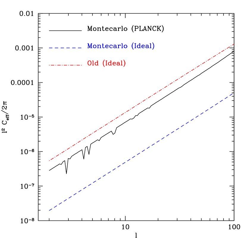
FIG. 8.: Comparison between $C_{l}^{eff}$ and the noise of our old method. We show the results for the Planck satellite and an ideal experiment. For our old method there was no difference in the noise between Planck and an ideal experiment on these angular scales.

In figure 8 we compare $1/C^{eff}_{l}$ to $W^{2}(l)({1\over N_{l}^{\cal S\cal S}}+{1\over N_{l}^{\cal E\cal E}})$. We show the results for two separate examples, an ideal experiment with no noise and infinite resolution and the Planck satellite. We focus on the large scale limit and for the ideal experiment we only consider the information coming from modes with $l<3000$. There are several salient features of the comparison. Although the difference between the methods is not so large for Planck it is much larger for the ideal experiment. This can be easily understood. In our previous method the power spectrum of the CMB noise in this limit was,

$$N_{l}^{\cal S\cal S}=(2\pi){\int l^{5}dl\ (C_{l}^{\tilde{T}\tilde{T}})^{2}\over(\int l^{3}dl\ C_{l}^{\tilde{T}\tilde{T}})^{2}}.$$ (70)

It is clear from equation (70) that once we get into the damping tail where the $C_{l}^{\tilde{T}\tilde{T}}$ fall exponentially, $N_{l}^{\cal S\cal S}$ no longer changes which means that our method does not receive any information from those modes. In contrast equation (68) shows that the amplitude of the $C_{l}^{\tilde{T}\tilde{T}}$ cancels in $C^{eff}_{l}$ as long as the modes had been measured with high $S/N$. Thus the new method continues to extract information from modes in the damping tail. In most practical cases this is not very important because the detector noise quickly dominates in this regime and then all methods downweight the modes. This explains why the difference between the two methods is not that large for Planck. There is another relevant consideration. When computing the variance we assumed that the field was only mildly non-Gaussian and that we could take the unlensed temperature power spectrum to calculate it. This is clearly not the case on small scales. As we have shown in previous sections, on small scales the fluctuations become very non-Gaussian as most of the power is generated by lensing. We only consider modes with $l<3000$ for the calculation of $C^{eff}_{l}$ to partially take into account this effect.

A The four point function

In the first part of this paper we have studied one particular physical limit when we are trying to recover information on the fluctuations of the mass distribution on scales much smaller than the coherence length of the CMB. To recover this limit we have to consider a quadrilateral in which two sides are much smaller that the other two (figure 9a). The two small sides correspond to the low pass filtered derivatives while the large $l$ correspond to the high passed filtered one. We consider the case where $l_{1},l_{2}\ll l_{3}\sim l_{4}$. As we noted before the power spectrum of the primary anisotropies decreases exponentially while that of the deflection angle is only as a power law. We conclude that of all the terms in equation (53) only those explicitly written dominate,

$$T_{4}(\hbox{\boldmath{$l$}}_{1},\hbox{\boldmath{$l$}}_{2},\hbox{\boldmath{$l$}}_{3},\hbox{\boldmath{$l$}}_{4})\approx 2{\hbox{\boldmath{$l$}}_{3}\cdot\hbox{\boldmath{$l$}}_{1}\ \hbox{\boldmath{$l$}}_{3}\cdot\hbox{\boldmath{$l$}}_{2}\over l_{3}^{2}}C^{\delta\delta}_{l_{3}}C^{\tilde{T}\tilde{T}}_{l_{1}}C^{\tilde{T}\tilde{T}}_{l_{2}},\ \ l_{1},l_{2}\ll l_{3}\sim l_{4},$$ (71)

where we approximated $C^{\delta\delta}_{l_{3}}\approx C^{\delta\delta}_{l_{4}}$.

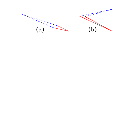
FIG. 9.: Quadrilaterals corresponding to the two limits discussed in the text. Panel a corresponds to configurations relevant for the cross correlation between the large scale gradient and the small scale power. Panel b shows the configurations that enter in the calculation of $\cal S$ and $\cal E$.

A different set of quadrilaterals dominate in the calculation of $\cal E$ and $\cal S$. Those variables extract information about the large scale $\kappa$ fluctuations from small angular scale fluctuations in the CMB. If we focus on modes of the temperature on scales larger that the damping tail $l^{2}C_{l}^{\tilde{T}\tilde{T}}$ remains approximately constant while the power spectra of the deflection angle falls. Moreover $\cal S$ and $\cal E$ are combination of derivatives of the CMB and the extra $l$s weigh the contribution to smaller scales. The power spectra of $\cal S$ and $\cal E$ are dominated by the type of quadrilaterals shown in figure 9b. All the $l$s are large but the quadrilaterals are thin. The thin diagonal corresponds to the $l$ of the $\kappa$ mode being recovered. The terms in equation (53) proportional to $C^{\tilde{T}\tilde{T}}_{l_{1}}C^{\tilde{T}\tilde{T}}_{l_{2}}C^{\delta\delta}_{l_{12}}$ (where $l_{1}$ and $l_{2}$ represent the length of the sides and $l_{12}$ is the small diagonal) dominate.

To extract all the information in the four point function we can add all the quadrilaterals with an appropriate weight,

$$\hat{Z} = {A_{f}\over(2\pi)^{2}}\int{d^{2}\hbox{\boldmath{$l$}}_{1}\over A_{l}}{d^{2}\hbox{\boldmath{$l$}}_{2}\over A_{l}}{d^{2}\hbox{\boldmath{$l$}}_{3}\over A_{l}}\beta({\cal S})\ T(\hbox{\boldmath{$l$}}_{1})T(\hbox{\boldmath{$l$}}_{2})T(\hbox{\boldmath{$l$}}_{3})T(\hbox{\boldmath{$l$}}_{4}),$$ (72)

where $\hbox{\boldmath{$l$}}_{4}=-(\hbox{\boldmath{$l$}}_{1}+\hbox{\boldmath{$l$}}_{2}+\hbox{\boldmath{$l$}}_{3})$ and $A_{l}$ is the area in $l$ space we are using. For the optimal filter that minimizes S/N one gets $\beta\propto T_{4}/C^{\tilde{T}\tilde{T}}_{l1}C^{\tilde{T}\tilde{T}}_{l2}C^{\tilde{T}\tilde{T}}_{l3}C^{\tilde{T}\tilde{T}}_{l4}$, where we have assumed Gaussianity to compute the variance. For the $S/N$ we get,

$$({S\over N})^{2} = {A_{f}^{-1}\over 24(2\pi)^{4}}\int{d^{2}\hbox{\boldmath{$l$}}_{1}}{d^{2}\hbox{\boldmath{$l$}}_{2}}{d^{2}\hbox{\boldmath{$l$}}_{3}}{T_{4}^{2}(\hbox{\boldmath{$l$}}_{1},\hbox{\boldmath{$l$}}_{2},\hbox{\boldmath{$l$}}_{3},\hbox{\boldmath{$l$}}_{4})\over C_{l1}^{\tilde{T}\tilde{T}}C_{l2}^{\tilde{T}\tilde{T}}C_{l3}^{\tilde{T}\tilde{T}}C_{l4}^{\tilde{T}\tilde{T}}},$$ (73)

where the power spectra in the denominator should include the contribution form detector noise.

We change integration variables in equation (73) and write,

$$({S\over N})^{2} = A_{f}^{-1}\int{d^{2}\hbox{\boldmath{$l$}}_{1}}({4C_{l1}^{\kappa\kappa}\over\tilde{C}^{eff}_{l}})^{2}$$ (74)

$$({1\over\tilde{C}^{eff}_{l}})^{2} = {1\over 24}\int{d^{2}\hbox{\boldmath{$l$}}_{2}\over(2\pi)^{2}}{d^{2}\hbox{\boldmath{$l$}}_{3}\over(2\pi)^{2}}{T_{4}^{2}(\hbox{\boldmath{$l$}}_{1}-\hbox{\boldmath{$l$}}_{2},\hbox{\boldmath{$l$}}_{2},\hbox{\boldmath{$l$}}_{3},-\hbox{\boldmath{$l$}}_{1}-\hbox{\boldmath{$l$}}_{3})\over C_{\hbox{\boldmath{$l$}}1-\hbox{\boldmath{$l$}}2}^{\tilde{T}\tilde{T}}C_{l2}^{\tilde{T}\tilde{T}}C_{l3}^{\tilde{T}\tilde{T}}C_{\hbox{\boldmath{$l$}}1+\hbox{\boldmath{$l$}}3}^{\tilde{T}\tilde{T}}(4C_{l1}^{\kappa\kappa})^{2}}.$$ (75)

This is a useful change of variables because it makes the integral resemble what we had in our old method. In this way the limit $l_{1}\rightarrow 0$ corresponds to quadrilaterals that have four large sides but a small diagonal ($\hbox{\boldmath{$l$}}_{1}$). Equation (6) of [7] reads,

$$({S\over N})^{2}=A_{f}^{-1}\int d^{2}\hbox{\boldmath{$l$}}{(4C_{l}^{\kappa\kappa})^{2}\over\sigma_{C_{l}}^{2}},$$ (76)

with $\sigma_{C_{l}}^{-2}=\sigma^{-2}_{C^{\cal S\cal S}_{l}}+\sigma^{-2}_{C^{\cal E\cal E}_{l}}+\sigma^{-2}_{C^{\cal S\cal E}_{l}}$.

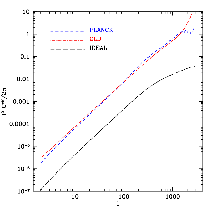
FIG. 10.: Result of Monte Carlo for 4pt function together with result from previous technique.

In figure 10 we compare the results $C_{l}^{eff}$ in (75) with $\sigma_{Cl}$ (76). The plot is qualitatively similar to figure 8 for the three point function. While there are hardly any improvements in our previous method when we go from Planck to an ideal experiment, there are significant differences for the optimal filter which continues to gather information from the damping tail. For Planck the situation is different, both the optimal method and our old method obtain a similar amount of information from the data. Even though the optimal method is able to get information from the damping tail in the ideal case, this is unimportant for Planck because the finite size of the beam makes it impossible. The fact that our previous method seems to have slightly less noise than the optimal method when $l$ is a few hundred is most probably an artifact. The noise in our old method was calculated using a Gaussian approximation which se had seen braking down slightly in our simulations [8]. As for the three point function we only included modes of the temperature with $l<3000$ as the power generated by lensing is non-Gaussian so our estimate of the variance of $\hat{Z}$ is not valid on smaller scales.

In the limit $l_{1}\rightarrow 0$ the four point function becomes approximately,

$$T_{4}(\hbox{\boldmath{$l$}}_{1}-\hbox{\boldmath{$l$}}_{2},\hbox{\boldmath{$l$}}_{2},\hbox{\boldmath{$l$}}_{3},-\hbox{\boldmath{$l$}}_{1}-\hbox{\boldmath{$l$}}_{3})\approx-C_{l2}^{\tilde{T}\tilde{T}}C_{l3}^{\tilde{T}\tilde{T}}l^{2}_{1}C_{l1}^{\delta\delta}.$$ (77)

To obtain equation (77) we had to assume that $C_{l}^{\kappa\kappa}$ is a decreasing function of $l$ and that $C_{\hbox{\boldmath{$l$}}1-\hbox{\boldmath{$l$}}2}^{\tilde{T}\tilde{T}}\approx C_{l2}^{\tilde{T}\tilde{T}}$ and the equivalent formula for $l_{3}$. Both of these assumptions break down in some range of $l$s. For example, $C_{l}^{\kappa\kappa}$ has a peak at $l\sim 100$ and when $l_{2}$ is in the damping tale range, for finite $l_{1}$ there might be corrections due to the difference between $C_{\hbox{\boldmath{$l$}}1-\hbox{\boldmath{$l$}}2}^{\tilde{T}\tilde{T}}$ and $C_{l2}^{\tilde{T}\tilde{T}}$. We can still use this expression as a rough estimate to try to compare how the optimal $\beta$ compares with the weight used by our previous method. In this limit and for the quadrilaterals relevant for this statistic, the optimal $\beta$ is equivalent to multiplying each of the temperatures by $(C_{l}^{\tilde{T}\tilde{T}})^{1/2}/(C_{l}^{\tilde{T}\tilde{T}}+B^{2}_{l}N_{l}^{\tilde{T}\tilde{T}})$. Thus for a temperature power spectra that goes as $C_{l}^{\tilde{T}\tilde{T}}\propto l^{-2}$ and when detector noise is irrelevant, the optimal filter amounts to multiplying the temperatures by $l$, equivalent to taking derivatives. This is the reason our previous method is not far from optimal in situations where we can neglect detector noise and we are not trying to extract information form the damping tail of the CMB. As we mention when we discussed the 3pt function, on small enough scales our treatment of the noise breaks down because the power is dominated by the power generated by lensing. The Gaussian approximation for the noise will not be valid.

V Conclusions

We have studied the generation of power by gravitational lensing on small angular scales. We have shown that the power spectra of the anisotropies gives a measure of the spectrum of the deflection angle. The generated power is correlated with the size of the large scale gradient.

The generation of power can be understood by studying the lensing of the primary anisotropies by a cluster of galaxies. On the scales of a cluster the CMB can be assumed to be a simple gradient. Lensing generates a wiggle on top of the gradient that can be tens of $\mu K$. This signal will be large enough to be detected by a CMB experiment which targeted clusters with sufficient angular resolution, $\sim 1\ {\rm arcmin}$.

The lensing effect produced by the large scale structure of the universe can be separated from other secondary effects or from intrinsic CMB anisotropies at the last scattering surface by measuring the cross correlation between the map of the large scale gradient and the map of the small scale power. We have shown that this statistic has only a slightly smaller signal to noise than the measurement of the small scale power itself. The power generated by lensing dominates over the intrinsic fluctuations for $l\succsim 4000$.

We have calculated the three and four point function of the lensing field in the small angle limit. The cross correlation between large and small scales as well as the statistics introduced in [8] are particular combinations of the four point function of the temperature field. We have calculated explicitly the dependence of the three and four point functions on the CMB and deflection angle power spectra as well as on the shape of the configuration. It is fair to say that both the statistic introduced here and those used in [8] can be viewed as particular ways of compressing the information in the four point function that take into account the physical intuition coming from our understanding of the lensing effect. The lensing effect predicts a particular dependence of the four point function on configuration and scale that can be used to separate it from other non Gaussian signals.

We are grateful to Uros Seljak and Wayne Hu for very very useful discussions. M.Z. is supported by NASA through Hubble Fellowship grant HF-01116.01-98A from STScI, operated by AURA, Inc. under NASA contract NAS5-26555.

REFERENCES

- [1] Electronic address: uros@mpa-garching.mpg.de
- [2] Electronic address: matiasz@ias.edu
- [3] Jungman G., Kamionkowski M., Kosowsky A., and Spergel D. N. Phys. Rev. Lett., 76, 1007 (1996); ibid Phys. Rev. D 54, 1332 (1996); Bond J. R., Efstathiou G. & Tegmark M., Mon. Not. Roy. Astron. Soc., 291, 33 (1997); Zaldarriaga M., Spergel D. N. and Seljak U. aAstrophys. J. 488, 1 (1997); Tegmark M., Eisenstein D., Hu W. and A. de Olivera Costa, ApJ. 530, 133 (2000)
- [4] M. Zaldarriaga Phys. Rev. D 55, 1822 (1997)
- [5] Bernardeu F., Astron. & Astrophys. 432, 15 (1997); Bernardeu F., Astron. & Astrophys. 338 767 (1998)
- [6] Goldberg, D. M. and Spergel, D.N., astro-ph/9811251
- [7] U. Seljak and M. Zaldarriaga, Phys. Rev. Lett. 82, 2636 (1999)
- [8] M. Zaldarriaga and U. Seljak, Phys. Rev. D 59, 123507 (1999)
- [9] R. B. Metcalf and J. Silk, J. ApJ Lett. 492, L1 (1998)
- [10] Information on CBI can be found at http://astro.caltech.edu/ tjp/CBI/abstract.html
- [11] U. Seljak, ApJ. 463, 1 (1996)
- [12] U. Seljak and M. Zaldarriaga, Phys. Rev. D 60, 043504 (1999)
- [13] Cooray, A. and Hu, W. astro-ph/9910397 (ApJ in press)
- [14] U. Seljak and M. Zaldarriaga, astro-ph/9907254
- [15] L. Knox, Z. Haiman and M. Zaldarriaga, in preparation.
- [16] Numerical Recepies, W. Press et al., Cambridge University Press