Limits on the Density of Compact Objects from High Redshift Supernovae

Abstract

Due to the effects of gravitational lensing, the magnification distribution of high redshift supenovae can be a powerful discriminator between smooth dark matter and dark matter consisting of compact objects. We use high resolution N-body simulations in combination with the results of simulations with compact objects to determine the magnification distribution for a Universe with an arbitrary fraction of the dark matter in compact objects. Using these distributions we determine the number of type Ia SNe required to measure the fraction of matter in compact objects. It is possible to determine a 20% fraction of matter in compact objects with 100-400 well measured SNe at $z\sim 1$, assuming the background cosmological model is well determined.

1 Introduction

Current cosmological data indicates that the density of matter in the Universe is around $\Omega_{\rm m}\sim 0.3$ (in units of critical density). Of this, big bang nuclesynthesis requires 15–20% be in the form of baryons, with the rest in some other more exotic form. Even among the baryons only $\Omega_{*}\sim 0.01$ has been accounted for directly. The rest could be in warm gas (Cen & Ostriker 1999), or in compact objects such as brown dwarfs, white dwarfs, or neutron stars. The nonbaryonic dark matter could be composed of a smooth microscopic component, such as axions, or alternatively it may be composed of compact objects, such as primordial black holes (Crawford and Schramm 1982). Although compact objects have been searched for in our own halo using microlensing studies (see Sutherland 1999 for a review), results are as of yet inconclusive. While the most straightforward interpretation is that a large fraction of the halo (up to 100%) is composed of compact objects of roughly 0.5M_☉, other scenarios using existing stellar populations remain viable. The bottom line is that, at present, the form of the bulk of the dark matter remains unknown.

In recent years there have been tremendous advances in our ability to observe and characterize type Ia supernovae. In addition to dramatically increasing the number of SNe observed at high redshift, the intrinsic peak brightness of these supernovae is now thought to be known to within about 15%. These supernovae are thus excellent standard candles, and by measuring the spread in their observed brightnesses it may be possible to determine the nature of the lensing, and thereby infer the distribution of the lensing matter.

It has long been recognized that the lensing of SNe can be used to search for the presence of compact objects in the Universe (Linder, Schneider & Wagoner 1988; Rauch 1991). Since the amount of matter near or in the beam determines the amount of magnification of the image, the magnification distribution from many SNe can probe for the presence of compact objects in the Universe. If the Universe consists of compact objects, then on very small scales most of the light beams do not intersect any matter along the line of sight, resulting in a dimming of the image with respect to the filled-beam (standard Robertson-Walker) result. On occasion a beam comes very near a compact object, resulting in a tremendous brightening of the ensuing image. In such a Universe the magnification distribution will be sharply peaked at the empty beam value, and will possess a long tail towards large magnifications. The lensing is sensitive to objects with Einstein rings larger than the linear extent of the SNe (roughly $10^{15}$cm at their maximum, which gives a lower limit on the mass of the lenses of $10^{-2}$M_☉).

Lensing due to compact objects is not, however, the only way to modify the flux of a SN. Even smooth microscopic matter, such as the lightest SUSY particle or axions, are expected to clump on large scales. The effect on the magnification distribution depends on the clumpiness of the Universe. If the clumping of matter in the Universe is very nonlinear then all of the matter will reside in dense halos, and the filaments connecting them, and there will be large empty voids extending tens or even hundreds of megaparsecs in diameter. There will thus be a large probability that a given line of sight will be completely devoid of matter, and so will give a large demagnification (as compared to the pure Robertson-Walker result). A simple way to estimate the importance of this effect is to compare the rms scatter in magnification to the demagnification of an empty beam relative to the mean (given by the filled beam value). Both can be calculated analytically, the former as an integral over the nonlinear power spectrum, and the latter as an integral over the combination of distances. The result depends on the redshift of interest, but for most realistic models the rms is smaller than the empty beam value at $z{\mathbin{\lower 3.0pt\hbox{$\,\hbox to0.0pt{\raise 5.0pt\hbox{$\char 62\relax$}\hss}\mathchar 29208\relax\,$}}}1$. This means that, at least qualitatively, it should be possible to distinguish between compact objects and smoothly distributed matter at such redshifts.

In this letter we extend previous work in several aspects. First, we provide the formalism to investigate models with a combination of both compact objects and smooth dark matter. Although Rauch (1991) and Metcalf and Silk (1999) have explored the use of lensing of supernovae to detect compact objects, they concern themselves with distinguishing between two extreme cases: either all or none of the matter in compact objects. Our formalism allows us to address the more general question of how well the fraction of dark matter in compact objects can be measured with any given SN survey. Both baryonic and dark matter are dynamically significant and could contribute to the lensing signal. For example, we can imagine four simplistic scenarios, in which the baryonic and dark matter are each in one of two states: smoothly distributed or clumped into compact objects (with masses above $10^{-2}$M_☉). To distinguish among these cases we need to be able to differentiate between 0%, 20%, 80%, and 100% of the matter in compact objects.

Second, we use realistic cosmological N-body simulations (Jain, Seljak and White 1999) to provide the distribution of magnification for the smooth microscopic component. Previous works (Metcalf and Silk 1999; Holz and Wald 1998) make the simplifying assumption of an uncorrelated distribution of halos to determine this distribution. As shown in Jain et al. (1999; JSW99), there are differences in the probability distribution function (pdf) of magnification for models with different shapes of the power spectrum and/or different values of cosmological parameters. For example, open models exhibit large voids up to $z\sim 1$, and their pdf’s extend almost to the empty beam limit. On the other hand, flat $\Omega_{\rm m}$ models have less power (being normalized to the same cluster abundance), and are more linear at higher $z$, resulting in a more Gaussian pdf. These differences become particularly important when we consider models in which only a fraction of the total matter is in compact objects. Magnification distributions in such cases differ only weakly from the smooth matter case, and an accurate description of the pdf is of particular importance. Finally, we also discuss the cross-correlation of SN magnification with convergence reconstructed from shear or magnification in the same field. As will be presented in the discussion section, this can be used as a further probe of compact objects.

2 Magnification probability distribution

We wish to derive the magnification probability distribution function (pdf) in a Universe with both compact objects and smooth dark matter. We begin with the magnification pdf for smoothly distributed matter, $p_{\rm{LSS}}(\mu,z)$, since this background distribution is present in all cases. For convenience we define the magnification, $\mu$, to be zero at the empty beam value. We use the pdf’s computed from N-body simulations in JSW99, obtained by counting the number of pixels in a map that fall within a given magnification bin. We explicitly include the dependence of the pdf on the redshift of the source. The two main trends with increasing $z$ are an increase in the rms magnification, and an increasing Gaussianity of the pdf (see figure 15 in JSW99). As we increase $z$ we are superimposing more independent regions along the line of sight, and the resulting pdf approaches a Gaussian by the central limit theorem.

A possible source of concern is that the resolution limitations of the N-body simulations might corrupt the derived pdf’s in ways which crucially impact our results. In principle we would like to resolve all scales down to the scale of the SN emission region ($10^{15}$cm in linear size). Fortunately such high resolution is unnecessary, as there is very little power in the matter correlation function on such small scales. The contribution to the second moment of the magnification peaks at an angular scale of $\theta>3^{\prime}$ (see figure 8 in JSW99); scales smaller than this do not significantly change the value of the second moment. These smaller scales, however, are relevant for the high magnification tail of the distribution, and even the largest N-body simulations are resolution limited in the centers of halos. As high magnification events are very rare in the small SN samples being considered, limitations in the resolution of the high magnification tail of the distribution are not of great concern. The simulations are very robust around the peak of the magnification pdf, with lower resolution PM simulations giving results in good agreement with higher resolution $P^{3}M$ simulations (figure 20 in JSW99). As these $P^{3}M$ simulations converge for the 2nd moment we may conclude that, aside from the high-magnification tail, the pdf’s obtained from these simulations do not suffer from the limitations of finite numerical resolution. This is also confirmed by smoothing the map by a factor of two, and comparing the pdf’s before and after the smoothing. The resulting pdf’s are very similar for all models, indicating that small scale power has little effect on the region of most interest, near the peak of the pdf.

The pdf’s are shown in figure 1, plotted against deviations from the mean magnification, $\delta\mu=\mu-\bar{\mu}$ ($\delta\mu=0$ corresponds to the mean (filled beam) value). The mean magnification, $\bar{\mu}$, is given by the difference between the empty beam and the mean (filled) beam values, which for SN at $z=1$ is $\bar{\mu}=0.24$ for $\Omega_{\rm m}=1$, $\Omega_{\lambda}=0$ models such as standard CDM model (with $\Omega_{\rm m}h=0.5$) or $\tau$CDM model (with $\Omega_{\rm m}h=0.21$), $\bar{\mu}=0.13$ for $\lambda$CDM model with $\Omega_{\rm m}=0.3$, $\Omega_{\lambda}=0.7$, and $\bar{\mu}=0.09$ for open (OCDM) model with $\Omega_{\rm m}=0.3$, $\Omega_{\lambda}=0$.

In contrast, in a Universe filled with a uniform comoving density of compact objects the pdf depends on a single parameter, the mean magnification $\bar{\mu}$, or equivalently, the mean convergence $\sigma$. The two are related via $\bar{\mu}=(1-\sigma)^{-2}-1$ ($\bar{\mu}\sim 2\sigma$ if $\sigma\ll 1$). The pdf rises sharply from $\mu=0$, and drops off as $\mu^{-3}$ for high $\mu$ (Paczyński 1986). Based on Monte-Carlo simulations, Rauch (1991) gives a fitting formula for the pdf:

$$p_{\rm C}(\mu,\sigma)=2\sigma_{\rm{eff}}\left[{1-e^{-b\mu}\over(1+\mu)^{2}-1}\right]^{3/2},$$ (1)

where $b=247e^{-22.3\sigma}$ and $\sigma_{\rm{eff}}$ is chosen so that the pdf integrates to unity. Note that this expression is only valid for $\sigma<0.1$, and can only be used for SN with $z<1$–2, depending on the cosmology.

To combine the two distributions we consider a model where a fraction $\alpha$ of the matter is in compact objects, and where these compact objects trace the underlying matter distribution. Suppose a given line of sight has magnification $\mu$ in the absence of compact objects. In the presence of compact objects the mean magnification along this line of sight remains unchanged. Since the smooth component contributes a SN magnification of $(1-\alpha)\mu$, the effect of compact objects is described with a pdf that gives a mean magnification of $\alpha\mu$. The combined pdf, $p(\mu)$, is given by integrating over the whole distribution,

$$p(\mu;\alpha,z)=\int_{0}^{{\mu\over 1-\alpha}}p_{\rm{LSS}}(\mu^{\prime},z)p_{\rm C}[\mu-\mu^{\prime}(1-\alpha),\alpha\mu^{\prime}/2]d\mu^{\prime}.$$ (2)

The middle panel in figure 1 shows the magnification pdf for a range of values of $\alpha$, for a cosmological model with $\Omega_{\rm m}=0.3$, $\Omega_{\lambda}=0.7$, and $\sigma_{8}=0.9$. The larger the value of $\alpha$, the closer the peak of the distribution to the empty beam value. As $\alpha$ increases from zero the pdf becomes wider, as the compact objects increase the large magnification tail. As $\alpha$ increases beyond $\alpha=0.2$, however, the distribution begins to narrow, since more and more lines of sight are empty and thus closer to the empty beam value. Note in particular the similarity between the $\alpha=0.2$ pdf and the $\tau$CDM model with $\alpha=0$ (upper panel in figure 1).

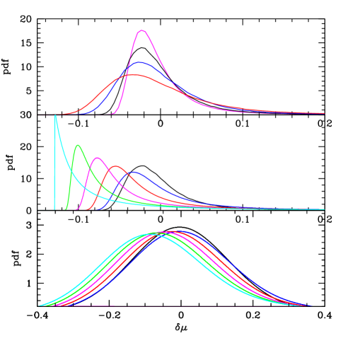
Figure 1: One point distribution function of magnification relative to the mean. The top panel shows the pdf’s in the absence of compact objects for (from top to bottom) OCDM (open), $\lambda$CDM, $\tau$CDM and standard CDM Universes (see JSW99 for a detailed description of the models). In the middle panel the pdf’s are given as a function of the fraction of total matter in compact objects, $\alpha$, for the $\lambda$CDM model. The curves from right to left are for $\alpha=0,0.2,0.4,0.6,0.8,1$. The bottom panel gives the same pdf’s as the middle one, convolved with the (intrinsic and observational) “noise” of the SNe ($\sigma_{\mu}=0.14$).

We need to further convolve these distributions with the measurement noise and the scatter in the intrinsic SN luminosities. Current estimates for these is 0.07 magnitudes for rms observational noise and 0.12 magnitudes for intrinsic scatter. The two combined give an additional rms scatter in magnification of 0.14 (Hamuy et al. 1996). To model this noise we convolve all the pdf’s with a Gaussian of width $0.14$. The resulting pdf’s are shown in the bottom panel of figure 1. The distinction between the different values of $\alpha$, although small, is still apparent. In the next section we calculate how many SNe are required to distinguish between the different curves in the bottom panel, and thereby measure $\alpha$.

3 Maximum Likelihood Analysis

We assume that the SNe are independent events. The likelihood function for the combined sample is then just the product of the individual SN likelihood functions,

$$L(\alpha)=\Pi_{i}p(\mu_{i};\alpha,z_{i}).$$ (3)

Redshift information could serve as an important confirmation that the effects observed are due to gravitational lensing, since the shapes and positions of the pdf’s evolve with redshift in a known manner. This redshift dependence does not, however, significantly increase the statistical power of the determination, compared to a sample where all of the SNe are at the mean redshift of the sample. To simplify the analysis we therefore assume that all of the SN are at a fixed redshift, z=1, and drop the redshift dependence of $p$. Taking the log and ensemble averaging we find

$$\langle\ln L(\alpha)\rangle = \Big{\langle}\sum_{i}\ln p(\mu_{i};\alpha)\Big{\rangle}$$ (4)

$$= N_{\rm SN}\int p(\mu;\alpha_{0})\ln p(\mu;\alpha)d\mu,$$

where $N_{\rm SN}$ is the number of observed SNe and $\alpha_{0}$ is the assumed true value of $\alpha$.

An estimate of the unknown parameter $\alpha$ is given by maximizing the log-likelihood function. The ensemble average of this gives the solution $\alpha=\alpha_{0}$ (i.e. the estimator is asymptotically unbiased). The error on the determination of the parameter $\alpha$ is given by the curvature of the negative log-likelihood function around its maximum. The ensemble average of this minimum variance is

$$\sigma_{\alpha}^{-2} = \Big{\langle}\Big{[}{\partial\ln L(\alpha)\over\partial\alpha}\Big{]}^{2}\Big{\rangle}$$ (5)

$$= N_{\rm SN}\int p(\mu;\alpha)\Big{[}{\partial\ln p(\mu;\alpha)\over\partial\alpha}\Big{]}^{2}d\mu,$$

which is to be evaluated at $\alpha=\alpha_{0}$. According to the Cramér-Rao theorem, $\sigma_{\alpha}$ gives the smallest attainable error on $\alpha$ for an unbiased estimator. As expected, the error decreases as the inverse square root of the number of SNe. Equation 5 determines the number of SNe required to achieve a given level of confidence in the measurement of $\alpha$, given a true value $\alpha=\alpha_{0}$. The case of $\alpha_{0}=0$ gives the sensitivity in the case of a Universe with a small fraction of matter in compact objects. In this case, for $\lambda$CDM model we find $\sigma_{\alpha}\sim 1.4N_{\rm SN}^{-1/2}$. This includes information from the full pdf, so any large differences between the models in the tail of the pdf would be statistically significant. Although this tail is susceptible to systematic effects generated by a lack of knowledge of the pdf, it will not be probed by small numbers of SNe. To exclude the tails we redid the integral in equation 5 including only the information within $\pm 2\sigma_{\mu}$ around the mean. The resulting error increases to $\sigma_{\alpha}\sim 1.8N_{\rm SN}^{-1/2}$. This means that we need on the order of 100 SNe to determine $\alpha$ to 20%, and around 1000 to determine $\alpha$ to 5%, all with one-sigma errors and assuming $\alpha_{0}=0$. The variance gradually increases with $\alpha_{0}$, and at $\alpha_{0}=1$ the required number of SN increases by a factor of 2.

The variance in $\alpha$ scales roughly linearly with the rms noise variance $\sigma_{\mu}$, so if the scatter in SN is larger the corresponding error in $\alpha$ increases. Variance also scales roughly inversely with the separation between mean and empty beam $\bar{\mu}$. For an open Universe, $\bar{\mu}$ is $7/10$ the value in the flat ($\Omega_{\rm m}=0.3$) Universe, so one needs roughly twice the number of SNe to reach the same sensitivity. For a flat Universe with $\Omega_{\rm m}=1$ and $\bar{\mu}=0.24$ the statistical significance increases, and one needs one quarter the SNe for the same sensitivity.

One can also test for the systematic effects introduced by using an incorrect model for the smooth component. To do this we did an analysis of a $\lambda$CDM Universe, “mistakenly” assuming it was an OCDM one. This results in a bias on the parameter $\alpha$ which can be as high as 20%, so that a precision test with this method is only possible once the parameters of the cosmological model are known precisely.

4 Discussion

Results obtained in the previous section indicate that high-$z$ SNe can enable an accurate determination of the fraction of matter in compact objects. If the estimates of the errors used here are reasonable, around 100 SNe at $z=1$ are required to make a 20% determination of the fraction of dark matter in compact objects. Although such numbers of SNe are not currently available, they can be expected in the near future as the high-redshift supernovae surveys continue their observations. Our results are in broad agreement with the results of Metcalf and Silk (1999), who find that about 50-100 SN are required to distinguish $\alpha=0$ from $\alpha=1$ with $90\%$ confidence. An important limitation will be systematic effects caused by uncertainties in the magnification distributions. For the smooth component these can be obtained using high resolution N-body simulations. We have argued that our results are reliable in the regime of application and can in any case be verified with higher resolution simulations in the future. Lack of knowledge of the underlying cosmological model may also introduce systematic effects, but again this can be expected to be better determined in the future.

Another important systematic error is our ignorance of the intrinsic dispersion in brightness of the observed SNe. Our simple assumption of a Gaussian noise profile in the measurement of the peak luminosities of SN Ia’s is certain to break down at some level. This noise estimate is based upon phenomenological observations of SNe, and needs to be borne out both by further observations (especially at low redshift, where lensing effects are negligible and independent calibrations are available) and by theoretical models. Deviations from Gaussian noise are most likely to be important in the tail of the magnification pdf’s, which can be excluded in the analysis. The lack of a precise knowledge of the intrinsic peak values of the SNe is less likely to cause a shift in the peak of the magnification pdf’s, which is the main signature of the lensing effect.

A further source of concern is redshift evolution of the intrinsic properties of the SNe. It is possible that both the mean and the higher moments of the distribution of peak luminosities of type Ia SNe varies with redshift, and this could pose significant challenges to an accurate measurement of lensing effects. Improvements in the determination of such effects will occur as the size of the data sets at both low and high redshifts are increased, and direct comparisons of observations are available. An important consistency check will be to demonstrate that the shift of the peak of the distribution as a function of redshift is consistent with theoretical expectations (under the assumed value of $\alpha$).

A complimentary method to obtain the pdf due to the background smooth matter component is to use weak lensing observations. This would provide the pdf directly from data, avoiding entirely the need for cosmological simulations. As discussed in §2 most of the power is on scales larger than 3’, so the pdf will almost converge to the correct one even if one smoothes the beam at this scale. Weak lensing surveys can provide maps of the magnifications by reconstructing the projected mass density from the shear extracted using galaxy ellipticities. The distribution of magnifications gives a pdf convolved with the random noise from galaxy ellipticities. Given an rms ellipticity of $0.4$, we find that about 50 galaxies per square arcminute are required to give an rms noise comparable to the noise in the SNe. This number is similar to the density of galaxies at deep ($m_{I}\sim 26$) exposures. Such galaxies have a mean redshift ($z\sim 1$) comparable to the SNe under discussion. We can therefore choose the size of a patch such that its rms noise agrees with the noise in the SN data. Such a pdf can then be directly compared to that from a SN sample (provided the differences in the redshift distribution are not too large), and any differences between the weak lensing and SN pdf’s would indicate the presence of compact objects or some other source of small scale fluctuation in magnification. Note that one cannot test for compact objects by simply using cross-correlation of the two magnifications, as compact objects do not change the mean magnification in a given line of sight, and thus the cross-correlation coefficient remains unchanged. The increased scatter, however, could provide the desired signature.

In conclusion, the magnification distribution from several hundred high redshift type Ia SNe has the statistical power to make a 10-20% determination of the fraction of the dark matter in compact objects. It remains to be seen whether this statistical power can be exploited at its maximum, or whether systematic effects will prove to be too daunting.

- (1) Cen R., Ostriker, J. P., 1999, ApJ, 514, L1
- (2) Crawford M., Scramm D. N., 1982, Nature, 298, 538
- (3) Hamuy M., et al., 1996, AJ, 112, 2398
- (4) Holz D. E., Wald R. M., 1998, Phys. Rev. D, 58, 3501
- (5) Jain B., Seljak U., White S., 1999, ApJ, in press (astro-ph/9901191, JSW99)
- (6) Linder E. V., Schneider P., Wagoner R. V., 1988, ApJ, 324, 786
- (7) Metcalf R. B., Silk J., 1999, ApJ, 519, L1
- (8) Paczyński B., 1986, ApJ, 304, 1
- (9) Perlmutter S. 1999, private communication
- (10) Rauch K., 1991, ApJ, 374, 83
- (11) Sutherland W., 1999, Rev. Mod. Phys, 71, 421