An exact Riemann Solver for multidimensional special relativistic hydrodynamics

Abstract

We have generalised the exact solution of the Riemann problem in special relativistic hydrodynamics [6] for arbitrary tangential flow velocities. The solution is obtained by solving the jump conditions across shocks plus an ordinary differential equation arising from the self-similarity condition along rarefaction waves, in a similar way as in purely normal flow. The dependence of the solution on the tangential velocities is analysed. This solution has been used to build up an exact Riemann solver implemented in a multidimensional relativistic (Godunov-type) hydro-code.

¹Departament d’Astronomia i Astrofísica, U. València, 46100 Burjassot, Spain
² MPI für Astrophysik, Karl-Schwarzschild-Str. 1, 85748 Garching, Germany

e-mail: jose.a.pons@uv.es

1 Introduction

The decay of a discontinuity separating two constant initial states (Riemann problem) has played a very important role in the development of numerical hydrodynamic codes in classical (Newtonian) hydrodynamics after the pioneering work of Godunov [2]. Nowadays, most modern high-resolution shock-capturing methods [5] are based on the exact or approximate solution of Riemann problems between adjacent numerical cells and the development of efficient Riemann solvers has become a research field in numerical analysis in its own (see, e.g., [14]).

Riemann solvers began to be introduced in numerical relativistic hydrodynamics at the beginning of the nineties and, presently, the use of high-resolution shock-capturing methods based on Riemann solvers is considered as the best strategy to solve the equations of relativistic hydrodynamics in nuclear physics (heavy ion collisions) and astrophysics (stellar core collapse, supernova explosions, extragalactic jets, gamma-ray bursts). This fact has caused a rapid development of Riemann solvers for both special and general relativistic hydrodynamics [3, 8].

The main idea behind the solution of a Riemann problem (defined by two constant initial states, $L$ and $R$, at left and right of their common contact surface) is that the self-similarity of the flow through rarefaction waves and the Rankine-Hugoniot relations across shocks allow one to connect the intermediate states $I_{*}$ ($I=L,R$) with their corresponding initial states, $I$. The analytical solution of the Riemann problem in classical hydrodynamics [1] rests on the fact that the normal velocity in the intermediate states, $v^{n}_{I_{*}}$, can be written as a function of the pressure $p_{I_{*}}$ in that state (and the flow conditions in state $I$). Thus, once $p_{I_{*}}$ is known, $v^{n}_{I_{*}}$ and all other unknown state quantities of $I_{*}$ can be calculated.

In the case of relativistic hydrodynamics the same procedure can be followed [6, 9], the major difference with classical hydrodynamics stemming from the role of tangential velocities. While in the classical case the decay of the initial discontinuity does not depend on the tangential velocity (which is constant across shock waves and rarefactions), in relativistic calculations the components of the flow velocity are coupled through the presence of the Lorentz factor.

2 The equations of relativistic hydrodynamics

The equations of relativistic hydrodynamics admit a conservative formulation which has been exploited in the last decade to implement high-resolution shock-capturing methods. In Minkowski space time the equations in this formulation read

$$\partial_{t}{\bf U}+\partial_{i}{\bf F}^{(i)}=0$$ (1)

where ${\bf U}$ and ${\bf F}^{(i)}({\bf U})$ ($i=1,2,3$) are, respectively, the vectors of conserved variables and fluxes

$${\bf U}=(D,S^{1},S^{2},S^{3},\tau)^{T}$$ (2)

$${\bf F}^{(i)}=(Dv^{i},S^{1}v^{i}+p\delta^{1i},S^{2}v^{i}+p\delta^{2i},S^{3}v^{i}+p\delta^{3i},S^{i}-Dv^{i})^{T}.$$ (3)

The conserved variables (the rest-mass density, $D$, the momentum density, $S^{i}$, and the energy density $\tau$) are defined in terms of the primitive variables,$(\rho,v^{i},\varepsilon)$, according to

$$D=\rho W~{},\quad S^{i}=\rho hW^{2}v^{i}~{},\quad\tau=\rho hW^{2}-p-D$$ (4)

where $W=(1-v^{2})^{-1/2}$ is the Lorentz factor and $h=1+\varepsilon+p/\rho$ the specific enthalpy.

In the following we shall restrict our discussion to an ideal gas equation of state with constant adiabatic exponent, $\gamma$, for which the specific internal energy is given by

$$\varepsilon=\frac{p}{(\gamma-1)\rho}.$$ (5)

3 Relation between the normal flow velocity and pressure behind relativistic rarefaction waves

Choosing the surface of discontinuity to be normal to the $x$-axis, rarefaction waves are self-similar solutions of the flow equations depending only on the combination $\xi=x/t$. Getting rid of all the terms with $y$ and $z$ derivatives in equations (1) and substituting the derivatives of $x$ and $t$ in terms of the derivatives of $\xi$, the system of equations can be reduced to just one ordinary differential equation (ODE) and two algebraic conditions

$$\rho hW^{2}(v^{x}-\xi)dv^{x}+(1-\xi v^{x})dp=0$$ (6)

$$hWv^{y}=\mbox{constant}$$ (7)

$$hWv^{z}=\mbox{constant},$$ (8)

with $\xi$ constrained by

$$\xi = \frac{v^{x}(1-c_{s}^{2})\pm c_{s}\sqrt{(1-v^{2})[1-v^{2}c_{s}^{2}-(v^{x})^{2}(1-c_{s}^{2})]}}{1-v^{2}c_{s}^{2}},$$ (9)

because non-trivial similarity solutions exist only if the Wronskian of the original system vanish. We have denoted by $c_{s}$ the speed of sound, provided by the equation of state. The plus and minus sign correspond to rarefaction waves propagating to the right (${\cal R}_{\rightarrow}$) and left (${\cal R}_{\leftarrow}$), respectively. The two solutions for $\xi$ correspond to the maximum and minimum eigenvalues of the Jacobian matrix associated to ${\bf F}^{(x)}({\bf U})$ [3, 8], generalizing the result found for vanishing tangential velocity [6].

From equations (7) and (8) it follows that $v^{y}/v^{z}=$ constant, i.e., the tangential velocity does not change direction across rarefaction waves. Notice that, in a kinematical sense, the Newtonian limit ($v^{i}\ll 1$) leads to $W=1$, but equations (7) and (8) do not reduce to the classical limit $v^{y,z}=$ constant, because the specific enthalpy still couples the tangential velocities. Thus, even for slow flows, the Riemann solution presented in this paper must be employed for thermodynamically relativistic situations ($h\gg 1$). The same result can be deduced from the Rankine-Hugoniot relations for shock waves (see next section).

Using (9) and the definition of the sound speed, the ODE (6) can be written as

$$\frac{dv^{x}}{dp}=\pm\frac{c_{s}}{W^{2}\gamma p}\frac{1}{\sqrt{1+g(\xi_{\pm},v^{x},v^{t})}}$$ (10)

where $v^{t}=\sqrt{(v^{y})^{2}+(v^{z})^{2}}$ is the absolute value of the tangential velocity and

$$g(\xi_{\pm},v^{x},v^{t})=\frac{(v^{t})^{2}(\xi_{\pm}^{2}-1)}{(1-\xi_{\pm}v^{x})^{2}}.$$ (11)

Considering that in a Riemann problem the state ahead of the rarefaction wave is known, equation (10) can be integrated with the constraint $hWv^{t}=$ constant, allowing to connect the states ahead ($a$) and behind ($b$) the rarefaction wave. The solution is only a function of $p_{b}$ and can be stated in compact form as

$$v^{x}_{b}={\cal R}^{a}_{\rightleftharpoons}(p_{b}).$$ (12)

4 Relation between post-shock flow velocities and pressure for relativistic shock waves.

The Rankine-Hugoniot conditions relate the states on both sides of a shock and are based on the continuity of the mass flux and the energy-momentum flux across shocks. Their relativistic version was first obtained by Taub [11] (see also [12, 4]).

Considering the surface of discontinuity as normal to the $x$-axis, the invariant mass flux across the shock can be written as

$$j\equiv W_{s}D_{a}(V_{s}-v^{x}_{a})=W_{s}D_{b}(V_{s}-v^{x}_{b}).$$ (13)

where $V_{s}$ is the coordinate velocity of the hyper-surface that defines the position of the shock wave and $W_{s}$ is the correspondent Lorentz factor, $W_{s}=(1-V_{s}^{2})^{1/2}$. According to our definition, $j$ is positive for shocks propagating to the right. In terms of the mass flux, $j$, the Rankine-Hugoniot conditions are

$$[v^{x}]=-\frac{j}{W_{s}}\left[\frac{1}{D}\right],$$ (14)

$$[p]=\frac{j}{W_{s}}\left[\frac{S^{x}}{D}\right],$$ (15)

$$\left[{hWv^{y}}\right]=0,$$ (16)

$$\left[{hWv^{z}}\right]=0,$$ (17)

$$[v^{x}p]=\frac{j}{W_{s}}\left[\frac{\tau}{D}\right].$$ (18)

Equations (16) and (17) imply that the quantity $hWv^{y,z}$ is constant across a shock wave and, hence, that the orientation of the tangential velocity does not change. The latter result also holds for rarefaction waves (see §3). Equations (14), (15) and (18) can be manipulated to obtain $v^{x}_{b}$ as a function of $p_{b}$, $j$ and $V_{s}$. Using the relation $S^{x}=(\tau+p+D)v^{x}$ and after some algebra, one finds

$$v^{x}_{b}=\left(h_{a}W_{a}v^{x}_{a}+\frac{W_{s}(p_{b}-p_{a})}{j}\right)\left(h_{a}W_{a}+(p_{b}-p_{a})\left(\frac{W_{s}v^{x}_{a}}{j}+\frac{1}{\rho_{a}W_{a}}\right)\right)^{-1}.$$ (19)

The final step is to express $j$ and $V_{s}$ as a function of the post-shock pressure. First, from the definition of the mass flux we obtain

$${V_{s}^{\pm}=\frac{\rho_{a}^{2}W_{a}^{2}v^{x}_{a}\pm|j|\sqrt{j^{2}+\rho_{a}^{2}W_{a}^{2}(1-{v_{a}^{x}}^{2})}}{\rho_{a}^{2}W_{a}^{2}+j^{2}}}$$ (20)

where $V_{s}^{+}$ ($V_{s}^{-}$) corresponds to shocks propagating to the right (left).

Second, from the Rankine-Hugoniot relations and the physical solution of $h_{b}$ obtained from the Taub adiabat [13] (the relativistic version of the Hugoniot adiabat), that relates only thermodynamic quantities on both sides of the shock, the square of the mass flux $j^{2}$ can be obtained as a function of $p_{b}$. Using the positive (negative) root of $j^{2}$ for shock waves propagating towards the right (left), the desired relation between the post-shock normal velocity $v^{x}_{b}$ and the post-shock pressure $p_{b}$ is obtained. In a compact way the relation reads

$$v^{x}_{b}={\cal S}^{a}_{\rightleftharpoons}(p_{b}).$$ (21)

We refer to the interested reader to references [6, 9] for further details.

5 The solution of the Riemann problem with arbitrary tangential velocities.

The time evolution of a Riemann problem can be represented as:

$$I\;\rightarrow\;L\;{\cal W}_{\leftarrow}\;L_{*}\;{\cal C}\;R_{*}\;{\cal W}_{\rightarrow}\;R$$ (22)

where $\cal W$ denotes a simple wave (shock or rarefaction), moving towards the initial left ($\leftarrow$) or right ($\rightarrow$) states. Between them, two new states appear, namely $L_{*}$ and $R_{*}$, separated from each other through the third wave $\cal C$, which is a contact discontinuity. Across the contact discontinuity pressure and normal velocity are constant, while the density and the tangential velocity exhibits a jump.

As in the Newtonian case, the compressive character of shock waves (density and pressure rise across the shock) allows us to discriminate between shocks ($\cal S$) and rarefaction waves ($\cal R$):

$${\cal W}_{\leftarrow\;(\rightarrow)}=\left\{\begin{array}[]{rcl}{\cal R}_{\leftarrow\;(\rightarrow)}&,&p_{b}\leq p_{a}\\ {\cal S}_{\leftarrow\;(\rightarrow)}&,&p_{b}>p_{a}\end{array}\right.$$ (23)

where $p$ is the pressure and subscripts $a$ and $b$ denote quantities ahead and behind the wave. For the Riemann problem $a\equiv L(R)$ and $b\equiv L_{*}(R_{*})$ for ${\cal W}_{\leftarrow}$ and ${\cal W}_{\rightarrow}$, respectively.

The solution of the Riemann problem consists in finding the positions of the waves separating the four states and the intermediate states, $L_{*}$ and $R_{*}$. The functions ${\cal W}_{\rightarrow}$ and ${\cal W}_{\leftarrow}$ allow one to determine the functions $v^{x}_{R*}(p)$ and $v^{x}_{L*}(p)$, respectively. The pressure $p_{*}$ and the flow velocity $v^{x}_{*}$ in the intermediate states are then given by the condition

$$v^{x}_{R*}(p_{*})=v^{x}_{L*}(p_{*})=v^{x}_{*}.$$ (24)

which is an implicit algebraic equation in $p_{*}$ and can be solved by means of an iterative method. When $p_{*}$ and $v^{x}_{*}$ have been obtained, the equation of state gives the specific internal energy and the remaining state variables of the intermediate state $I_{*}$ can be calculated using the relations between $I_{*}$ and the respective initial state $I$ given through the corresponding wave.

Notice that the solution of the Riemann problem depends on the modulus of $v^{t}$, but not on the direction of the tangential velocity. Figure 1 shows the solution of a particular Riemann problem [10] for different values of the tangential velocity $v^{y}=0,0.5,0.9,0.99$. The crossing point of any two lines in the upper panel gives the pressure and the normal velocity in the intermediate states. Whereas the pressure in the intermediate state can take any value between $p_{L}$ and $p_{R}$, the normal flow velocity can be arbitrarily close to zero in the case of an extremely relativistic tangential flow.

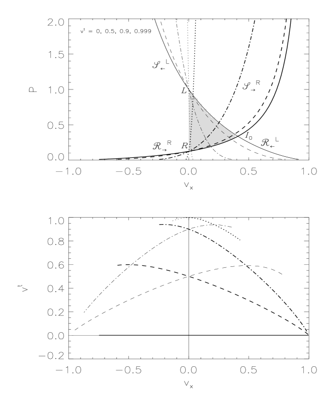
Figure 1: Graphical solution in the $(p,v^{x})$–plane (upper panel) and in the $(v^{t},v^{x})$–plane (lower panel) of the relativistic Riemann problem with initial data $p_{L}=1.0$, $\rho_{L}=1.0$, $v^{x}_{L}=0.0$; $p_{R}=0.1$, $\rho_{R}=0.125$ and $v^{x}_{R}=0.0$ for different values of the tangential velocity $v^{t}=0,0.5,0.9,0.999$, represented by solid, dashed, dashed-dotted and dotted lines, respectively. An ideal gas EOS with $\gamma=1.4$ was assumed. The crossing point of any two lines in the upper panel gives the pressure and the normal velocity in the intermediate states. The value of the tangential velocity in the states $L_{*}$ and $R_{*}$ is obtained from the value of the corresponding functions at $v^{x}$ in the lower panel, and $I_{0}$ gives the solution for vanishing tangential velocity. The range of possible solutions is given by the shaded region in the upper panel.

To study the influence of tangential velocities on the solution a Riemann problem, we have calculated the solution of a standard test involving the propagation of a relativistic blast wave produced by a large jump in the initial pressure distribution for different combinations of tangential velocities [9]. Although the structure of the solution remains unchanged for different tangential velocities, the values in the constant state may change by a large amount.

Figure 2: Exact (solid lines) and numerical profiles along the diagonal of pressure (squares), density (crosses) and normal velocity (diamonds) for the 2–dimensional relativistic shock tube discussed in the text.

6 Discussion and conclusions.

We have obtained the exact solution of the Riemann problem in special relativistic hydrodynamics with arbitrary tangential velocities. Unlike in Newtonian hydrodynamics, tangential velocities are coupled with the rest of variables through the Lorentz factor, present in all terms in all equations. It strongly affects the solution, especially for ultra-relativistic tangential flows. In addition, the specific enthalpy also acts as a coupling factor and modifies the solution for the tangential velocities in thermodynamically relativistic situations (energy density and pressure comparable to or larger than the proper rest-mass density), rendering the classical solution incorrect in slow flows with very large internal energies.

Our solution has interesting practical applications. First, it can be used to test the different approximate relativistic Riemann solvers and the multi-dimensional hydrodynamic codes based on directional splitting. Second, it can be used to construct multi-dimensional relativistic Godunov-type hydro codes. As an example, we have simulated a relativistic tube [10], in a $100\times 100$ Cartesian grid, where the initial discontinuity was located in a main diagonal. The initial states were $\rho_{L}=10$, $\rho_{R}=1$, $p_{L}=13.3$, $p_{R}=0.66E-3$, $v_{L}=0$, $v_{R}=0$, and the adiabatic index is $\gamma=5/3$. Spatial order of accuracy was set to second order by means of a monotonic piecewise linear reconstruction procedure and second order in time is obtained by using a Runge-Kutta method for time advancing. The exact solution of the Riemann problem is used at every interface to calculate the numerical fluxes. The results are shown in Figure 2, and are comparable to those obtained with other HRSC methods. Profiles of all variables are stable and discontinuities are well resolved without excessive smearing. An efficient implementation of this exact Riemann solver in the context of multidimensional relativistic PPM [7] is in progress and will be reported elsewhere.

References

- [1] Courant, R. and Friedrichs, K. O. (1948), Supersonic Flows and Shock Waves, Interscience.
- [2] Godunov, S. K. (1959), A Finite Difference Method for the Numerical Computation and Discontinuous Solutions of the Equations of Fluid Dynamics, Mat. Sb., 47, 271.
- [3] Ibañez, J.M. & Martí, J.M. (1999), Riemann Solvers in Relativistic Astrophysics, J. Comput. Appl. Math., in press.
- [4] Königl, A. (1980), Relativistic Gas Dynamics in Two Dimensions, Phys. Fluids., 23, 1083.
- [5] LeVeque, R.J. (1992), Numerical Methods for Conservation Laws (Second Edition), Birkhäuser.
- [6] Martí, J.M. & Müller, E. (1994), The Analytical Solution of the Riemann Problem in Relativistic Hydrodynamics, J. Fluid Mech., 258, 317.
- [7] Martí, J.M. & Müller, E. (1996), Extension of the Piecewise Parabolic Method to One-Dimensional Relativistic Hydrodynamics, J. Comput. Phys. 123, 1.
- [8] Martí, J.M. & Müller, E. (1999) Numerical Hydrodynamics in Special Relativity, Living Reviews in General Relativity, in press; also astro-ph/9906333.
- [9] Pons, J.A., Martí, J.M. & Müller, E. (1999), The Exact Solution of the Riemann Problem with non-zero tangential velocities in Relativistic Hydrodynamics, J. Fluid Mech., submitted.
- [10] Sod, G. A. (1978), A Survey of Several Finite Difference Methods for Systems of Nonlinear Hyperbolic Conservation Laws, J. Comp. Phys., 27, 1.
- [11] Taub, A. H., (1948), Relativistic Rankine-Hugoniot Relations, Phys. Rev., 74, 328.
- [12] Taub, A. H., (1978), Relativistic Fluid Mechanics, Ann. Rev. Fluid Mech., 10, 32.
- [13] Thorne, K. S. (1973), Relativistic Shocks: The Taub Adiabat, Astrophys. J., 179, 897.
- [14] Toro, E. (1998), Riemann Solvers, Springer.