An XMM pre-view of the cosmic network: galaxy groups and filaments

Abstract

A large fraction of the baryons today are predicted to be in hot, filamentary gas, which has yet to be detected. In this paper, we use numerical simulations of dark matter and gas to determine if these filaments and groups of galaxy will be observable be XMM. The simulated maps include free-free and line emission, galactic absorption, the XMM response function, photon noise, the extragalactic source distribution, and vignetting. A number of cosmological models are examined as well as a range of very simple prescriptions to account for the effect of supernovae feedback (preheating). We show that XMM has a good chance of observing emission from strong filaments at $z\sim 0.1$. This becomes much more difficult by $z\sim 0.5$. The primary difficulties lie in detecting such a large, diffuse object and in selecting an appropriate field. We also describe the range of group sizes that XMM should be sensitive to (both for detection and spectral analysis), although this is more dependent on the unknown nature of the feedback. Such observations will greatly improve our understanding of feedback and should also provide stronger cosmological constraints.

1 Introduction

The filamentary large scale distribution of matter in the universe is a consequence of the gravitational instability of a medium that was relatively smooth in early times, with the non-linear patterns we see today having evolved from small density fluctuations. There have been two competing stories for the formation of structures: the (Russian) pancaking picture ([Zel’dovich 1970]) and the (Western) hierarchical clustering picture ([Peebles 1980]). The “cosmic web” paradigm ([Bond et al 1996]) reconciles these two scenarios, showing that the final-state is actually present in embryonic form in the overdensity pattern of the initial fluctuations, with nonlinear dynamics just sharpening the image. This has several immediate applications to observations, in particular: superclusters are predominantly cluster-cluster bridges and the strongest filaments exist between aligned clusters.

The study of galaxy clusters has undergone spectacular developments in the last decade, ranging from the galaxy content to the detailed physics of the hot intra-cluster gas (ICM) and also addressing the question of the large scale distribution of clusters. Conversely, intermediate density structures, that we would define as density contrasts of the order of $\delta\rho/\rho\sim 4$, i.e. loose galaxy groups and filaments, have captured less attention so far. The main reason being their comparatively humble appearance in the optical or X-ray sky.

However, both theory and simulations indicate that a better knowledge of the filaments will improve our understanding of cosmology. Many current models suggest that a large fraction of the baryons at low redshift should be in filaments (e.g. [Miralda-Escudé et al. 1996]; [Cen & Ostriker 1999]). Heated to a temperature intermediate between that of hot clusters and cool voids, this would imply that presently most of the baryons remain undetected. Moreover, the overall cosmic network - best underlined by the numerous groups and filaments - may show different topologies depending on the value of the cosmological parameters and the nature of dark matter.

Filaments and groups are superb laboratories for studying the effects of galaxies on their environment and, in turn, the impact of this environment on galaxy evolution. The velocity dispersion of groups and filaments ($\sim$ 400 km/s) is larger than the internal velocities of galaxies themselves, thus interactions are frequent and the intragroup gas should have very similar properties to the neighbouring filamentary gas. Feedback from galaxy/star formation is expected to play a major role — much more, probably, than for massive clusters where gravitational physics may be sufficient to explain the bulk of their properties. Also, many quasars are thought to be in groups and may have significant effects on their environment. In the various observed X-ray/optical correlations, groups tend to show a larger dispersion than clusters (e.g. [Mulchaey & Zabludoff 1998]). There are also some systematic difference in the general properties of clusters and groups ([Renzini 1997]). These results certainly suggest that galaxies play an important role in groups and filaments, but this process is very poorly understood. This is one of the compelling arguments in favor of deep and extended X-ray surveys: a large sample of groups (free of projection effects or of any optical selection biases, which can be very stringent e.g. “compact” groups) would enable the statistical study of their temperatures and abundances to be further compared with their optical properties and theoretical predictions. Since groups occupy the intermediate range in the cosmic mass function — between clusters and galaxies — a better understanding of their global properties would provide an alternative view of the missing link between quasi-linear and extremely non-linear systems.

Our observational knowledge of the truly filamentary medium is even slimmer than for groups, bordering on non-existent. Attempts to detect the “supercluster” or filament gas directly from its bremsstrahlung emission have led to very marginal or negative results so far ([Briel & Henry 1995]; [Wang et al. 1997]; [Kull & Böhringer 1999]; see also [Markevitch 1999]). Although the temperature of this gas is expected to be around 1 keV, its low density considerably limits its potential emissivity in the X-ray or EUV band. It is thus primarily a technical challenge to observe this warm component which is predicted to account for some 20-40% of the total baryonic mass by redshift $z=0$ ([Cen & Ostriker 1999]). In addition to a direct window into the physics of this medium, closely connected with the cooler components such as Ly$\alpha$ clouds and galaxies, quantitative observations would put an upper limit to the contribution of filaments to the auto-correlation function of the X-ray background.

Thanks to its unrivaled sensitivity, XMM is to open a new era in the [0.1-10] keV range. One aspect of the mission is focussed on high resolution spectroscopy, the other main one being the observation of faint extended diffuse emission. In the EPIC imaging mode at 1 keV, XMM has a Half Power Diameter of 13” on-axis, a collecting area of 2600 cm² and an energy resolution of 20%. Beside the detailed study of massive clusters of galaxies, XMM is thus ideally suited to search for low surface brightness extended structures such as very distant galaxy clusters (at redshifts substantially greater than one, if they exist!) or groups and filaments out to a redshift close to unity.

XMM instruments are now fully calibrated and the launch is scheduled for the end of the millennium. It is thus timely to investigate carefully which of the issues related to intermediate density structures can be efficiently addressed by XMM. This will have a direct impact on the preparation of dedicated observations as well on their analysis. In order to provide quantitative arguments, we have simulated XMM images. The X-ray emissivity of a filamentary region at a range of redshifts was computed from high resolution hydrodynamical simulations combined with a detailed plasma code and folded with the XMM spectral and imaging responses. We present here the XMM simulated images and further discuss the physics that could be extracted from them.

The paper is organized as follows. In the next section, we present the hydrodynamical code and the various cosmological models and epochs that were chosen for the the simulations. Section 3 describes how the X-ray images were produced. The general discussion on the detectability of groups and filaments is given in Section 4 as well as practical hints for future large surveys of groups. In the conclusion we present further observational prospects in connection with other wavelengths.

2 The AMR simulations

2.1 Basic ingredients of the simulations

In order to generate realistic XMM images, we have performed a series of cosmological simulations incorporating both dark matter and baryonic gas. The method used is an adaptive mesh refinement (AMR) algorithm that models the dark matter with particles and the gas with a series of meshes. More complete descriptions of the method are available elsewhere ([Bryan & Norman 1997]; [Norman & Bryan 1999]), but we briefly outline it here. An initial grid was set up at high redshift with density and velocity fields drawn from a power spectrum appropriate for the cosmology of interest. The particles were initialized using the Zel’dovich approximation. The equations of hydrodynamics were solved on the mesh using the piecewise parabolic method ([Colella & Woodward 1984]; [Bryan et al. 1995]). Since the mesh is fixed, gravitational collapse inevitably causes structures to shrink to sizes comparable to the mesh spacing, causing inaccuracies. AMR solves this problem by identifying regions which need enhanced resolution and laying down a finer mesh over those volumes. The solution is interpolated onto this finer grid — which typically has cell sizes half as large — and an improved solution is computed there. The process can be repeated as necessary and a hierarchy of grids is generated, with cell sizes varying as small as necessary (up to a predefined limit in order to limit the cpu time required).

In Table 1, we list the parameters of the simulations performed. They are drawn from three different cosmologies: 1) a standard cold dark matter (SCDM) model, in order to link with previous work on this model, 2) a cosmological constant-dominated universe ($\Lambda$CDM), which agrees with the majority of current observational data, and 3) a tilted-CDM (tCDM) model. Together, these three choices should provide a good range in the currently viable parameter space.

In addition to changing the cosmology, we also experimented with additional physical processes in the simulations. In some simulations we included a simple equilibrium cooling-curve ([Sarazin & White 1987]) (although we should note that the spatial resolution of these simulations, 50 $h^{-1}$ kpc, were not sufficient to fully resolve the cooling instability). The physical state of the intergalactic medium is intimately linked with galaxy formation (through galactic outflows) and hence star formation and supernovae. In fact, simulations of clusters (e.g. [Navarro, Frenk & White 1996]; [Bryan & Norman 1998]) show that gravity and adiabatic gas physics alone do not correctly predict the luminosity-temperature relationship. Instead of the observed relation which is approximately $L_{X}\sim T^{3}$, they predict $L_{X}\sim T^{2}$. The difference is most likely due to feedback from stars ([Kaiser 1991]; [Balogh, Babul & Patton 1999]), which those simulations did not include. We would like to take into account the effect of feedback here, unfortunately the input of energy from supernovae and stellar winds is technically difficult to include properly in simulations ([Metzler & Evrard 1994]). In place of a full treatment, we attempt to include this effect by pre-heating the gas, effectively setting a minimum entropy (see also Navarro, White and Frenk 1996). This does not have a large effect on the hot gas in the outskirts of clusters which, due to shocking, naturally has a high entropy. However, it does produce a larger core radius, decreasing the central gas density compared to a simulation without pre-heating. This decreases the luminosity of small clusters and groups (since the X-ray emissivity is proportional to the square of the density), and can reproduce the observed luminosity-temperature relationship. Since it is not clear what this initial entropy should be, we tried two cases: a mild feedback in which the initial gas temperature is set to $4\times 10^{7}$ K at $z=20$ (and would adiabatically cool to $9\times 10^{4}$ K by $z=0$ for a fluid element which follows the cosmic mean density without shocking), and a more extreme version in which the initial temperature is 5 times higher. The impact on the $L_{X}-T$ relationship of introducing galaxy feedback in the simulations is shown in Fig. 1. This form of “feedback” is successful in reproducing the observed relation. Clearly, a simple pre-heating of the gas does not produce the same energy distribution as the feedback from millions of massive stars; however the extremes adopted here (no feedback at all contrasted with heating the gas everywhere) will at least indicate which diagnostics are sensitive to the feedback and by how much.

Figure 1: The introduction of “mild” feedback (see text) in the simulations results in a decrease of the luminosity of small groups and, consequently, steepens the $L_{X}-T$ relationship in agreement with the observations: observations give $\sim L_{X}\propto T^{3}$ whereas $L_{X}\propto T^{2}$ is expected in the case of a pure gravitational collapse. The observed correlation appears to be very tight when “cooling flow” clusters are excluded ([Arnaud & Evrard 1999]) and shows no obvious evolution out to $z\sim 0.4$ ([Mushotzky & Scharf 1997])

The cosmological constant-dominated model we have selected is in good agreement with most available observational data, and in particular with the shape and evolution of the luminosity function. The flat, tCDM model is certainly less-favoured by the present data. It is consistent with the number-density of clusters and COBE measurements of the microwave background; however, it does not match with the many indications of a low-density universe, nor with the recent supernovae data implying the presence of a cosmological constant. We include it to indicate the range of variation that cosmology will introduce in our filament properties. The X-ray properties of the models are particularly important for this study and so in Figure 2, we plot the luminosity function for each model, as predicted from a simple Press-Schechter prescription combined with a relation between mass and temperature, coupled with the observed luminosity-temperature relation (see [Bryan & Norman 1998] for more details on this procedure). While both models agree at $z=0$, observations are now becoming available at much higher redshifts. For example, the lack of evolution out to $z\sim 0.8$ for moderate to high-luminosity clusters ([Rosati et al. 1998]) places tighter constraints on the models. In Figure 2 we also plot the predicted luminosity function at $z=0.8$. For the $\Lambda$CDM model, the lack of evolution is naturally predicted; however for the tCDM model to agree, we have to stretch the bounds of the observed evolution (or rather lack of evolution) of the luminosity-temperature relation, which is the most uncertain part of the modeling procedure. For example, using a very recent determination of the evolution of the $L_{X}-T$ relation ([Reichart, Castander & Nichol 1999]), the tCDM model disagrees at the 2 $\sigma$ level. Note, however, that the observational luminosity function at high redshift is still somewhat uncertain (see for example [Reichart et al. 1999], where a deficit of very high luminosity clusters is observed).

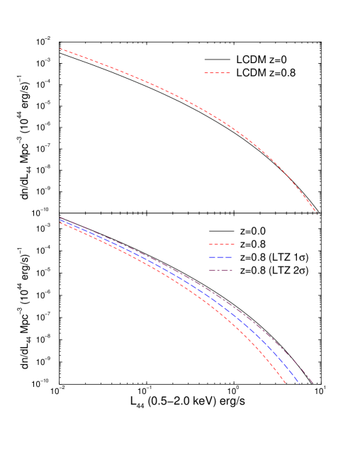
Figure 2: The predicted luminosity function of the $\Lambda$CDM (top) and tCDM (bottom) models at $z=0$ and $z=0.8$. In the bottom panel, we also show the effect of varying the amount of redshift evolution in the observed $L_{X}-T$ relation by one and two sigma. Since observations seem to indicate little or no evolution in the luminosity function, the tCDM model is marginally inconsistent.

Table 1: AMR simulation models - comoving cell size: (50 kpc/$h$)³

Model	$\sigma_{8}$	$h$	$\Omega_{matter}$	$\Omega_{\Lambda}$	$\Omega_{b}$	$n$	cooling?	“feedback”?
CDM	0.95	0.6	0.4	0.6	0.06	1.0	no	no
$\Lambda$CDMf1	0.95	0.6	0.4	0.6	0.06	1.0	no	mild
$\Lambda$CDMc	0.95	0.6	0.4	0.6	0.06	1.0	yes	no
$\Lambda$CDMcf1	0.95	0.6	0.4	0.6	0.06	1.0	yes	mild
$\Lambda$CDMf2	0.95	0.6	0.4	0.6	0.06	1.0	no	extreme
tCDM	0.6	0.5	1.0	0.0	0.06	0.81	no	no
SCDM	0.6	0.5	1.0	0.0	0.06	1.0	no	no

Table 2: Steps in the simulation of the XMM images

Step	Operation
0a	AMR cube + plasma code $->$ X-ray emissivity cube
0b	0a + XMM response + Exp. time $->$ photon cube
1a	projected photon cube
1b	1b + Poisson noise
2a	a single XMM field of view from 1a
2b	2a + extragalactic point sources

2.2 The extracted filament

Since we are primarily interested in the filament environment, we specifically selected such a region. This was done by initially simulating — at low resolution — a cube 100 $h^{-1}$Mpc on a side. The output was examined, and a volume 18 $\times$ 23 $\times$ 33 $h^{-3}$ Mpc³ was selected. This region lay between two large clusters and was the strongest filament in the box. In order to better sample the initial conditions, the simulation was rerun with an addition mesh of size 28x34x50 placed over the region. As many particles as grid points were used. The adaptive meshing was then turned on and a relatively high resolution simulation of this region was performed. The rest of the 100 $h^{-1}$ Mpc cube was again simulated at low resolution, which is sufficient to provide the necessary gravitational tidal field.

3 Simulations of the XMM images

From the temperature and density cubes, we have calculated for each simulation cell, the X-ray plasma emissivity using a redshifted Raymond-Smith code having a metallicity of 0.3 solar. The choice of this latter value - which is comparable to that of galaxy clusters, although the total production of heavy elements by group galaxies is certainly lower - has been guided by the fact that mixing and enrichment are probably more efficient than in clusters, the medium being much less dense. Then, assuming a given exposure time, we computed the photon numbers to be received from each cell by XMM taking into account the complete instrumental response (a composite matrix made of the responses of the 2 MOS CCDs and of the PN CCD in imaging mode folded with the X-ray telescope response). This was done for the [0.4-4] energy band, best suited for detecting structures having temperatures of the order of 1-2 keV; we do not consider the photons below 0.4 keV as diffuse emission is too much affected by galactic absorption. In the calculation, we assumed a galactic hydrogen column density of $N_{H}=5~{}10^{20}$cm². (Note that assuming a metallicity of 0.1 instead of 0.3 would decrease the count rate of a 2 keV group or of 1 keV filament by 10% or 40% respectively in the [0.4-4] keV band).

For each set of AMR simulations we thus obtained a “photon cube” which was in turn projected along the line of sight, i.e. the $x$ axis. The resulting photon image has a pixel size equal to the apparent size of the AMR cell seen at the simulation redshift (Table 2, step 1a); Poisson photon noise was then added to each pixel (step 1b). This is typically what an XMM wide angle survey would look like once the pointings have been placed side by side, all instrumental effects corrected, extragalactic point sources removed and the resulting image rebinned to increase the signal (note however, this is an ideal case without diffuse background). In a second step, we have simulated in more detail some individual pointings, focussing on a given area of the projected photon cube as would be seen by the circular XMM field of view of $\sim$ 30 arcmin. Practically, this consists of extracting a given sky region from step 1a, rebinning it with a pixel size of 4 arcsec and then applying the vignetting function allowing for Poisson statistics in each pixel (step 2a). Finally, we have introduced the extragalactic LogN-LogS source distribution ([Hasinger et al 1998]) assuming that all sources have a power law spectrum with a photon index of 2. Images of these pointlike sources have been convolved by the mean XMM/EPIC point spread function as a function of off-axis angle and randomly added to the filament sub-image together with a constant diffuse background rate of $10^{-5}$ count/s/pixel(4”) (step 2b). The instrumental characteristics used in the simulations are from the ground-based calibration phase (e.g. [Dahlem & Shartel 1999]).

Table 3: Simulated image parameters

step	redshift	pixel size	image size
		kpc & arcsec	pixels & arcmin
1	0.1	25/h     19”	$952\times 1392$     $295^{\prime}\times 432^{\prime}$
1	0.5	100/h     19”	$238\times 348$     $74^{\prime}\times 108^{\prime}$
2	0.1	$\sim$ 5/h     4”	$512\times 512$     $\o=34^{\prime}$
2	0.5	$\sim$ 20/h     4”	$512\times 512$     $\o=34^{\prime}$

In order to directly compare the filament emissivities at $z=0.1$ and $z=0.5$, we have rebinned the $z=0.1$ image obtained in step 1a with a pixel size 4 times smaller than the original simulation cell of 100/h kpc. In the calculations, we have neglected the $\sim 10\%$ difference in angular distance between the open and closed models at $z=0.5$.

4 Results

In order to study the effects of cosmology, distance and input physics on the detectability by XMM of groups and filaments, we display the simulated images of the entire filament, prior to including the back/foreground population of X-ray point sources. We first discuss the visibility of the $z=0.5$ case, then the $z=0.1$ one, as the larger apparent size of the diffuse structures is likely to make their detection more problematic, despite their proximity.

4.1 Global images at $z=0.5$

Fig. 8 shows the predicted XMM images for our three cosmological models, namely: standard CDM, tilted CDM and $\Lambda$CDM. As expected, the difference between open and closed models is striking. Conversely, the tCDM and SCDM models appear to be very similar in terms of X-ray emissivity, at least for the group population. This seems quite reasonable, since both were normalized at the 8 Mpc/h scale. In Fig. 9, we display four realizations of the $\Lambda$CDM model calculated under various heating or cooling assumptions as given in Table 1, to be compared to the $\Lambda$CDM model of Fig. 8.

Considering first the effect of cooling alone ($\Lambda$CDM   &   $\Lambda$CDMc models), groups appear substantially smaller in spatial extent when cooling is at work. This is because the cooling has reduced their pressure support, which keeps them extended. Moreover, the $\Lambda$CDM   &   $\Lambda$CDMc density maps shown in Figs. 3 & 4 indicate that the model with cooling has more small clumps, but most of them do not show up in the X-ray images: these are galaxy-sized objects, unresolved by the simulation. In these clumps, the gas can cool down to $10^{4}$K, which prevents most of them from emmiting in the X-ray band. In the larger groups however, the gas in the center is still hot enough to radiate and much denser than in the no-cooling case which makes their X-ray profile significantly more peaked.

2cm

Figure 3: Density cube for the $z=0.5~{}\Lambda$CDM model shown for an isosurface of $4~{}10^{-4}$ atom cm^-3

2cm

Figure 4: Density cube for the $z=0.5~{}\Lambda$CDMc model shown for an isosurface of $4~{}10^{-4}$ atom cm^-3

As discussed in Sec. 2.1, preheating raises the gas entropy prior to gravitational collapse, preventing high central densities by the formation of a larger core. This is best seen when considering the “extreme” feed back model ($\Lambda$CDMf2 Fig. 9): clusters are much more extended, and small objects are virtually absent. Group central densities are significantly lower than in the $\Lambda$CDM models, with only three clumps reaching the limiting density of $4~{}10^{-4}~{}$ atom cm^-3 (to compare with Figs. 3 & 4). Some of the gas which did not succeed in collapsing is now trapped in the filamentary structures which explains the higher emissivity of the diffuse region compared to any other models. Paradoxically, the average temperature in the filament is somewhat lower in $\Lambda$CDMf2 than in $\Lambda$CDM; this is due to the absence of shock-heating in the pre-heated filament gas. These effects are less pronounced if mild feedback is assumed.

Finally, we considered a mixed case, combining the effects of feedback plus cooling ($\Lambda$CDMcf1), likely to be the most realistic. This shows very little difference from that with feedback alone (contrary to the striking discrepancy between $\Lambda$CDM and $\Lambda$CDMc) suggesting that here the gas stays too hot and diffuse to cool. While none of these models captures the detailed dynamics of real stellar and galactic feedback, they do give an indication of the direction and amplitude of their effects.

4.2 Individual pointings at $z=0.5$

Figures 10 & 11 show the two individual pointings indicated on Fig. 9. Although groups as small as $10^{14}$ M_⊙ (or smaller depending on the model) will be visible for integration times as short as 10 ks, the diffuse filamentary gas seems not to be detectable even with 200 ks exposures. This is essentially due to the very low density of the filament (Fig. 5) and the high background level caused by source confusion. It is interesting to note that in all models the intra-filament gas is expected to have a temperature around 1 keV as can be appreciated on Fig. 6

2cm

Figure 5: Density cube for the $z=0.5~{}\Lambda$CDMcf1 model, shown for an isosurface of $5~{}10^{-5}$ atom cm^-3

2cm

Figure 6: Temperature cube for the $z=0.5~{}\Lambda$CDMcf1 model, shown for an isosurface of 1 keV

4.3 Global images at $z=0.1$

The apparent size of the same filament at $z=0.1$ is very large ($\sim 5^{o}\times 7^{o}$) and it would require more than 300 pointings to be entirely covered by XMM (assuming a spacing of 20’ per pointing to minimize the loss of sensitivity due to vignetting). Nevertheless, as for the $z=0.5$ models, we have calculated the number of photons to be collected by XMM from the entire structure for individual integration times of 200 ks. The results are summarized in Fig. 12 for the SCDM and $\Lambda$CDM models with or without cooling/heating. Compared with the corresponding $z=0.5$ images, one sees clearly the evolution of structure in terms of merging: small groups are flowing along the filaments to reach bigger entities located at the nodes.

4.4 Individual pointings at $z=0.1$

We have performed detailed simulations of two XMM fields specifically centered on filamentary segments (cf Fig. 12). The images are presented in Fig. 13 and suggest that, at this redshift, very faint details of the network will be detectable. These may include collapsing regions as well as pure diffuse filamentary emission.

5 Prospects for XMM observations

5.1 The “nb(photons) - Mass(groups)” relation

In order to get a better idea of the observability of the groups seen in these simulated XMM images, we show in Fig. 7 the relation between the mass of a group and the number of photons observed for the $\Lambda$CDM simulation at $z=0.5$. The number of photons measured comes from extracting each region above a given flux threshold from the photon cube. The mass is calculated by summing both the gas and the dark matter within a sphere whose mean density is about 300 times the mean density of the universe (see [Bryan & Norman 1998] for a more complete definition). A power law fit produces a slope of 0.59. Simple adiabatic scaling laws would indicate a relation like $M\sim L_{X}^{0.75}$, while our feedback simulations produce something like $M\sim L_{X}^{0.5-0.6}$. Note, however, that we do not directly measure the emissivity, but count individual photons to be detected by XMM in the [0.4-4] keV band (assuming $N_{H}=5~{}10^{20}~{}cm^{-2}$). The scatter in the relation is about 20%.

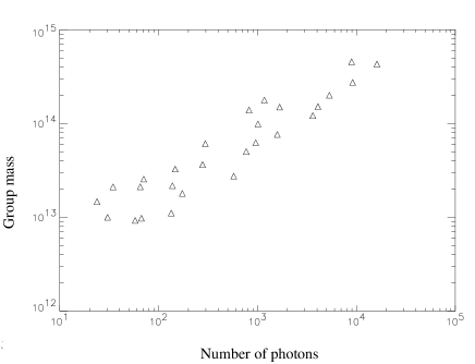
Figure 7: The relation between group mass at $z=0.5$ and the number of photons detected in the 0.4-4 keV range from a simulated 100 ks XMM image ($\Lambda$CDM model).

5.2 Shallow pointings

With exposure times as short as 10 ks, XMM will reach a sensitivity of $\sim 5~{}10^{-15}erg/s/cm^{2}$ in the [0.5-2] keV band for pointlike sources. Our simulations (Fig.11) show that at this limiting flux, objects having masses down to $10^{14}$ M_⊙ will be readily detectable out to $z\sim 0.5$. This includes all clusters and much of the group population. As indicated in Fig. 7, groups having masses of the order of $10^{14}$ M_⊙ will produce some 100 photons in 10 ks thus, enabling simple source extent characterization as can be appreciated in Fig. 11. More generally, with 10 ks exposures, the 3$\sigma$ detection threshold for extended sources having a characteristic size of about 1 arcmin ( i.e. a $2\times$ 250 kpc core radius seen at $z\sim 0.5-1$) is around 65 photons on-axis, which is 2 times higher than for pointlike sources ([Valtchanov et al 2000]).

In the previous section, we demonstrated that both preheating and cooling affects the detectability of small groups by making them either more centrally concentrated (radiative cooling) or more extended (preheating). Of course it should be kept in mind that preheating is simply our attempt to model stellar feedback. More sophisticated methods are being developed which attempt to account for the multi-phase nature of the flow ([Wu, Fabian & Nulsen 1998]; [Teyssier, Chieze & Alimi 1998]) as well as more complete models of galaxy formation and feedback (see for example [Yepes et al. 1997]; [Hultman & Pharasyn 1999]; [Martin 1999]). In developing and testing these methods, observational comparisons will play an important role. Therefore, a large shallow XMM survey would provide a unique data base to study, in a statistically complete way, the physics of groups.

5.3 Deep pointings

Assuming 200 ks exposures, XMM can reach a sensitivity of $\sim 10^{-16}erg/s/cm^{2}$ but will then face the generic problem of source confusion. The limiting flux where this is expected to occur corresponds to exposure times between 30-50 ks. The exact level will remain unknown until the first XMM or Chandra in-flight observations. This is due to the lack of previous deep high resolution observations above 2 keV (ASCA had a PSF of $\sim$ 3 arcmin). It is thus obvious that the main hurdle for studying diffuse emission (clusters or filaments) will be contamination by the point source population, rather than the limited number of photons. Note that, to the contrary, source confusion should barely be a problem for Chandra (PSF $\sim 1$ arcsec) but its much lower effective area makes the task of detecting filaments much more difficult.

An additional difficulty comes from the fact that the simulations have a finite thickness, which is not the case of the “observable” universe; thus, true confusion may be even worse than presented here because of the presence of fore/background filaments.

5.3.1 Groups

Assuming a 50% efficiency for the X-ray detection algorithm in measuring extended source fluxes and that a net minimum photon number of 1000 is necessary for spectral studies at low energies, Fig. 7 indicates that it will be possible to obtain temperature and abundance estimates for objects having masses down to $\sim 10^{14}M_{\odot}$ at $z=0.5$ (i.e. some 2000 photons collected during an exposure time of 200 ks). It should also be kept in mind that we are assuming that the X-ray emission from AGN and other galactic sources can be identified and removed from the group X-ray emission.

Such observations will be particularly important as it will provide new insights into the physics of low mass clusters and groups. For example, since supernovae are responsible for both adding energy and metals to the intergroup medium, a measurement of the metallicity helps to constrain the feedback history (which is even more important in groups than in clusters). Determinations of the baryon fraction can also cast light on the strength of feedback and the nature of group evolution.

5.3.2 Filaments

The detection of filamentary emission (and not simply of “supercluster gas”) is a real challenge for the next generation of X-ray satellites. With its unrivaled sensitivity and large field of view, XMM is a priori the best suited instrument. Our detailed simulations indicate that this will be very difficult at $z\sim 0.5$ whatever the assumed cosmology or heating/cooling processes, but possible at $z\sim 0.1$ for an open model associated with mild feedback ($\Lambda$CDMf1, Sec. 4.4).

More generally, in this work, we have tried to gauge the effect of uncertainties in our understanding of the physics of filament (i.e. cooling and feedback). We have shown that cooling alone tends to decrease somewhat the luminosity of filaments. This occurs because gas cools into many small clumps, reaching temperatures which are too low to radiate in the X-ray band. However, this also produces groups and clusters which are much brighter than observations indicate (as reflected in the mismatched $L_{X}-T$ relation).

On the other hand, in the simulation with the extreme form of preheating ($\Lambda$CDMf2), small groups are prevented from forming at all (in a more realistic simulation, these groups would form but then expel nearly all of their gas due to supernovae in galaxies). This causes more gas to end up in the filaments, improving their visibility.

The case of mild feedback, which satisfies all the observational constraints is intermediate in terms of filament emission. Feedback and cooling ($\Lambda$CDMcf1, the most likely model) appears very similar to the model with feedback alone ($\Lambda$CDMf1) in terms of emissivity. Thus, our prediction that filamentary emission will be detectable at $z\sim 0.1$ is likely to be robust. Note also that the variation due to changes in input physics is much smaller for filaments than for groups and filaments, which are more sensitive to the nature and strength of the feedback.

The number of photons received from the filament detectable in Fig. 13 (bottom) is $\sim$ 21000 for an integration time of 200 ks. This is, in principle, 10 times more than strictly necessary for measuring the temperature of the feature. However, the filament photons are spread over the entire detector and severely contaminated by the point source population (resolved or not). With the present analysis techniques, it is not possible to extract a workable spectrum.

5.4 Technical remark on filtering techniques

Multi-resolution filtering techniques give very good results for enhancing the signal from point source and cluster type emission as well as assessing the significance of the detected objects (cf Fig. 10 & 11). However, our preliminary processing shows that gaussian filtering is better adapted for enhancing very diffuse structures having a size comparable to that of the detector. In a forthcoming paper (Valtchanov et al 2000), we shall investigate further source detection and extraction techniques and the possibility of obtaining spectroscopic information from diffuse filamentary regions.

6 Conclusion. How can the cosmology be constrained?

We have presented detailed predictions as to the visibility of the cosmic structure by XMM using high resolution hydrodynamical simulations. Special attention has been paid to physical processes — in addition to pure gravitational infall and shocks — which can affect the X-ray emissivity. The discussion was focussed on the lowest density objects, i.e., small groups of galaxies and cosmic filaments.

One of the main conclusion is that the entire (or much of) the low mass group population will be visible with modest exposure times out to a redshift of one half, depending on the adopted cosmology and details of the physics. More specifically, for open universes, we have investigated two effects (cooling and feedback) using simplified prescriptions. We now place them in a more general context: (i) Feedback from galaxies, such as supernova driven galactic winds, is expected to be particularly efficient prior to group formation since the rather small masses of groups makes them more sensitive to the entropy of the gas from which they form. Energy and matter input to the ICM occurs throughout the lifetime of the group, but probably but with less impact on their luminosities than with the preheating adopted here ([Metzler & Evrard 1994]); (ii) Further, because of their lower temperatures, groups are to be also strongly affected by cooling. This process is essentially multi-phase and because of the condensation of cooling clouds, the remaining hot gas has an X-ray luminosity strongly reduced compared to what would be expected from an equivalent adiabatic group; the X-ray mass fraction is also significantly influenced by this multi-phase evolution. As we have emphasized in this work, neither of these effects are currently well understood or modelled.

The XMM group sample should then provide precious insights into these various mechanisms. However, a comprehensive analysis of the group population should necessarily also involve a combined optical study, since galaxy distributions and velocities are also key parameters in understanding the history of groups (an example is the so-called $\beta$ problem, e.g. [Gerbal et al 1994]).

While less numerous and significantly less affected by cooling or feedback, large clusters — the deepest potential wells in the universe — play an important role in our current cosmological constraints. For example, their number density provides the best estimate of the amplitude of the primordial density fluctuations at scales around 8$h^{-1}$ Mpc (e.g. [Viana & Liddle 1996]). Similarly, their evolution in redshift has been suggested by many authors as a way to measure the matter density of the universe. However, a convincing measurement of this has proven difficult due to the uncertain relation between a cluster’s mass and its X-ray luminosity. In fact, this has driven many workers to use the temperature, which is more difficult to measure, in addition to the luminosity since the former is more closely related to the mass (e.g. [Oukbir & Blanchard 1997]). Since much of the uncertainty in understanding cluster luminosities stems from feedback, the proposed observations for the low mass sample (along with improved modeling) will be able to cast light on such things as the $L_{X}-T$ relation, and so provide much tighter cosmological constraints.

Even more interesting, however, is the idea of using the spatial distribution of groups and filaments themselves to constrain cosmology. Even a cursory glance at Fig. 8 shows that the width, length and distribution of filaments is sensitive to cosmology (in fact, the dependence at $z=0$ is almost entirely on the amplitude of the power spectrum). The difficulty is extracting this information from the more realistic observations shown in later figures. One possibility is to use the location of small groups to trace out the filaments and apply topological measurements, such as the genus statistic. This has been done in the case of galaxies. A difficulty with this and other approaches is simply the weak signal of the filaments. In this paper we have shown that they are detectable with XMM, but confusion will be an issue. A promising approach to increase the signal-to-noise ratio is to combine multiple measurement techniques by cross-correlating galaxy surveys, X-ray maps and perhaps even microwave maps, to use the expected Sunyaev-Zel’dovich signal. This will help to eliminate the confusion caused by unrelated (and hence uncorrelated) sources. In the optical band, weak lensing analysis techniques are rapidly improving and it may soon become possible to measure the direct gravitational signal from the mass associated with filaments (preferentially located between two clusters). Having gained a better understanding of feedback and cooling mechanisms from the study of groups, we may then be in a position to interpret the observed X-ray emissivity in terms of density, temperature and abundances and hence infer the baryon fraction in filaments.

Acknowledgements:
Support for GLB was provided by NASA through Hubble Fellowship grant HF-01104.01-98A awarded by the Space Telescope Science Institute, which is operated by the Associate of Universities for Research in Astronomy, Inc., for NASA under contract NAS 5-26555. We thank the National Center for Supercomputing Applications for providing computational resources for some of the simulations carried in this work. We acknowledge useful conversations with Alexandre Refregier. We are grateful to H. Brunner and G. Hasinger for detailed information used in the XMM simulations.

Colour Fig. 8 to 13 and corresponding captions
are available at: http://www.mit.edu/$\sim$gbryan/xmm_preview.html

References

- [Allen & Fabian 1998] Allen S.W., Fabian A.C., 1998, MNRAS 297, L63-L68
- [Arnaud & Evrard 1999] Arnaud M., Evrard A., 1999, MNRAS 305, 631
- [Balogh, Babul & Patton 1999] Balogh M.L., Babul A. & Patton D.R. 1999, MNRAS, in press
- [Bond et al 1996] Bond R., Kofman L., Pogosyan D., 1996, Nature, 380, 603
- [Briel & Henry 1995] Briel, U.G. & Henry, J.P. 1995, A&A, 302, L9
- [Bryan et al. 1995] Bryan G.L., Norman M.L., Stone J.M., Cen R., Ostriker J.P., 1995, Comp. Phys. Comm. 89, 149-168
- [Bryan & Norman 1997] Bryan G.L., Norman M.L., 1997, in “Computational Astrophysics”, Proc. 12th Kingston Conference, Halifax, Oct. 1996, eds. D. Clarke & M. West (PASP), p. 363-368
- [Bryan & Norman 1998] Bryan G.L. & Norman M.L., 1998, ApJ, 495, 80
- [Cen & Ostriker 1999] Cen R. & Ostriker, J.P, 1999, ApJ, 514, 1
- [Colella & Woodward 1984] Colella P., Woodward P.R., 1984, J. Comp. Phys. 54, 174
- [Dahlem & Shartel 1999] Dahlem M. & Schartel N. 1999, The XMM Users Hanbook,http://astro.estec.esa.nl/XMM/user/uhb_top.html
- [Gerbal et al 1994] Gerbal D., Durret F., Lachi ze-Rey M., 1994, A& A 288, 746
- [Hasinger et al 1998] Hasinger G., Burg R., Giacconi R., Schmidt M., Trümper J., Zamorani G., 1998, A& A 329, 482
- [Hultman & Pharasyn 1999] Hultman, J. & Pharasyn A. 1999, A&A, 347, 769
- [Kaiser 1991] Kaiser N. 1991, ApJ, 383, 104
- [Kull & Böhringer 1999] Kull, A. & Börhigner, H. 1999, A&A, 341, 23
- [Markevitch 1999] Markevitch, M. 1999, ApJ, 522, L13
- [Martin 1999] Martin, C.L. 1999, ApJ, 513, 156
- [Metzler & Evrard 1994] Metzler, C.A., Evrard, A.E. 1994, ApJ, 437, 564
- [Miralda-Escudé et al. 1996] Miralda-Escudé, J., Cen, R., Ostriker, J.P. & Rauch, M. 1996, ApJ, 471, 582
- [Mulchaey & Zabludoff 1998] Mulchaey, J.S. & Zabludoff, A.I. 1998, ApJ, 496, 73
- [Mushotzky & Scharf 1997] Mushotzky R.F., Scharf C.A., 1997, ApJ Letters 482, L13
- [Navarro, Frenk & White 1996] Navarro J.F., Frenk. C.S., White S.D.M. 1996, ApJ, 462, 563
- [Norman & Bryan 1999] Norman M.L., Bryan G.L., 1999, to appear in “Numerical Astrophysics 1998”, eds. S. Miyama & K. Tomisaka, Tokyo, March 10-13, 1998
- [Oukbir & Blanchard 1997] Oukbir, J. & Blanchard, A. 1997, A&A, 317, 13
- [Peebles 1980] Peebles, P.J.E., 1980 Large Scale Structuree of the Universe (Princeton University Press)
- [Reichart, Castander & Nichol 1999] Reichart, D.E., Castander, F.J., Nichol, R.C. 1999, ApJ, 516
- [Reichart et al. 1999] Reichart, D.E., Nichol, R.C., Castander, F.J., Burke, D.J., Romer, A.K., Holden, B.P., Collins, C.A., Ulmer, M.P. 1999, ApJ, 518, 521
- [Renzini 1997] Renzini, A. 1997, ApJ, 488, 35
- [Rosati et al. 1998] Rosati, P. Della Ceca, R., Norman, C., Giacconi, R. 1998, ApJ, 492, 21L
- [Sarazin & White 1987] Sarazin C.L., White R.E. 1987, ApJ, 320, 32
- [Starck & Pierre 1998] Starck J.-L., Pierre M., 1998, A& A Sup., 128, 397
- [Teyssier, Chieze & Alimi 1998] Teyssier, R., Chieze, J.P., Alimi, J.M. 1998, in “Untangling Coma Berenices: A New Vision of an Old Cluster”, Proceedings of the meeting held in Marseilles (France), June 17-20, 1997, Eds.: Mazure, A., Casoli F., Durret F. , Gerbal D., Word Scientific Publishing Co Pte Ltd, p 149.
- [Valtchanov et al 2000] Valtchanov I., Gastaud R., Pierre M., Starck J.-L., 2000 A&A in preparation
- [Viana & Liddle 1996] Viana, P.T.P., Liddle, A. 1996, MNRAS, 281, 531L
- [Wang et al. 1997] Wang, Q. Daniel, Connolly, A., Brunner, R. ApJ, 487, 13L
- [Wu, Fabian & Nulsen 1998] Wu, K.K.S., Fabian, A.C., Nulsen, P.E.J. 1998, MNRAS, 301, 20L
- [Yepes et al. 1997] Yepes, G., Kates, R., Khokhlov, A., Klypin, A. 1997, MNRAS, 284, 235
- [Zel’dovich 1970] Zel’dovich, Ya. B. 1970, Astrofizika 6,319,