The nearby M-dwarf system Gliese~866 revisited

Abstract

We present an improved orbit determination for the visual pair in the M-dwarf triple system Gliese~866 that is based on new speckle-interferometric and HST observations. The system mass is $M=0.34\pm 0.03\,M_{\odot}$. The masses of the components derived using the mass-luminosity relation are consistent with this mass sum. All three components of Gliese 866 seem to have masses not far from the hydrogen burning mass limit.

1 Introduction

It is now a well established fact that there exists a large number of substellar objects (see e. g. the recent review article by Oppenheimer et al. Oppenheimer00 (2000)). This increases the need for a better understanding of stellar properties at the lower end of the main sequence. Nearby low-mass stellar systems are particularly important for this purpose, because their orbital motion allows dynamical mass determinations.
Here we will consider the nearby triple system Gliese~866 (Other designations: LHS 68, WDS 22385-1519). Using speckle interferometry, Leinert et al. (Leinert86 (1986)) and also McCarthy et al. (McCarthy87 (1987)) discovered a companion (henceforth Gliese~866 B) located about 0$\aas@@fstack{\prime\prime}$4 away from the main component Gliese~866 A. Following observations proved the possibility to cover the whole orbit of this binary system within a few years by speckle-interferometric observations. Based on 16 data points, Leinert et al. (Leinert90 (1990), hereafter L90) presented a first determination of orbital parameters and masses. They derived the combined mass of the system to be $0.38\pm 0.03\,M_{\odot}$. This was inconsistent with values of $M_{\mathrm{A}}\approx 0.14\,M_{\odot}$ and $M_{\mathrm{B}}\approx 0.11\,M_{\odot}$ obtained from empirical mass-luminosity relations and stellar interior models (see L90 and references therein).
In the meantime an additional spectroscopic companion (hereafter called Gliese~866 a) to Gliese~866 A has been detected (Delfosse et al. Delfosse99 (1999)). This is a plausible reason for the mentioned mass excess in Gliese~866, but – given the fact that only $0.38\,M_{\odot}$ now had to be distributed among three stars – raises the question for a substellar component in the Gliese~866 system.
To improve on the mass determination of the components of Gliese~866 we have taken 20 more speckle-interferometric observations and one additional HST determination of relative position. These show the orbit of the wide pair: B with respect to Aa. We present an overview of the observations and the data reduction process in Sect. 2. The results are given in Sect. 3, discussed in Sect. 4 and are summarized in Sect. 5.

2 Observations and data reduction

A list of the new observations and their results is given in Table 1. The observations numbered 1, 3, 5 and 7 used one-dimensional speckle-interferometry. Details of observational techniques and data reduction for this method are described in Leinert & Haas (Leinert89 (1989)).

Table 1: Results of new observations of Gliese~866. Position angle and projected separation are those of Gliese~866 B relative to Gliese~866 Aa. The abbreviations in column ”Telescope” denote Calar Alto (CA), Kitt Peak National Observatory (KPNO), European Southern Observatory (ESO) and New Technology Telescope (NTT). The latter has an aperture of 3.5 m.

No.	Date	Epoch	Position	Projected	Filter	$I_{\mathrm{B}}/I_{\mathrm{Aa}}$	Telescope	Camera
			angle [$\degr$]	separation			(see caption)
				[mas]
1	01.09.1990	1990.6681	348.0 $\pm$ 2.2	481 $\pm$ 18	K	0.58 $\pm$ 0.03	CA 3.5 m	1D
2	04.12.1990	1990.9254	339.8 $\pm$ 2.4	463 $\pm$ 19	K		KPNO 3.8 m	2D
3	19.09.1991	1991.7173	186.5 $\pm$ 3.4	186 $\pm$ 11	K	0.55 $\pm$ 0.02	CA 3.5 m	1D
4	29.10.1991	1991.8268	155.5 $\pm$ 3.8	200 $\pm$ 13	K	0.51 $\pm$ 0.03	CA 3.5 m	1 - 5 $\mu$m
5	16.05.1992	1992.3751	15.3 $\pm$ 0.5	244 $\pm$ 6	K	0.57 $\pm$ 0.05	ESO 3.6 m	1D
6	14.10.1992	1992.7885	350.8 $\pm$ 1.5	449 $\pm$ 11	K	0.58 $\pm$ 0.01	CA 3.5 m	1 - 5 $\mu$m
7	10.01.1993	1993.0273	348.6 $\pm$ 1.4	480 $\pm$ 12	K	0.55 $\pm$ 0.03	CA 3.5 m	1D
8	29.07.1993	1993.5750	319.3 $\pm$ 1.2	259 $\pm$ 11	K	0.618 $\pm$ 0.071	ESO NTT	SHARP
9	02.10.1993	1993.7529	277.7 $\pm$ 0.5	105 $\pm$ 4	K	0.60 $\pm$ 0.03	CA 3.5 m	MAGIC
10	01.05.1994	1994.3313	74.9 $\pm$ 2.7	126 $\pm$ 4	K	0.562 $\pm$ 0.031	ESO NTT	SHARP
11	14.09.1994	1994.7036	5.9 $\pm$ 0.4	327 $\pm$ 4	K	0.552 $\pm$ 0.009	CA 3.5 m	MAGIC
12	12.12.1994	1994.9473	354.0 $\pm$ 0.2	434 $\pm$ 4	K	0.551 $\pm$ 0.017	CA 3.5 m	MAGIC
13	13.12.1994	1994.9501	354.3 $\pm$ 0.3	439 $\pm$ 4	917 nm	0.603 $\pm$ 0.009	CA 3.5 m	MAGIC
14	09.07.1995	1995.5201	337.3 $\pm$ 0.3	439 $\pm$ 4	K	0.581 $\pm$ 0.014	ESO NTT	SHARP
15	16.08.1995	1995.6243	333.1 $\pm$ 0.3	392 $\pm$ 4	K	0.587 $\pm$ 0.022	ESO 3.6 m	SHARP 2
16	08.06.1996	1996.4381	131.6 $\pm$ 0.2	156 $\pm$ 1	583 nm	0.69 $\pm$ 0.06	HST	FGS3
17	27.09.1996	1996.7419	28.0 $\pm$ 0.5	188 $\pm$ 4	K	0.568 $\pm$ 0.022	CA 3.5 m	MAGIC
18	25.08.1997	1997.6489	340.2 $\pm$ 0.2	485 $\pm$ 4	K	0.593 $\pm$ 0.006	ESO 3.6 m	SHARP 2
19	16.11.1997	1997.8761	333.3 $\pm$ 0.1	391 $\pm$ 4	K	0.58 $\pm$ 0.01	CA 3.5 m	MAGIC
20	07.05.1998	1998.3477	214.8 $\pm$ 0.3	104 $\pm$ 7	K	0.558 $\pm$ 0.004	ESO NTT	SHARP
21	10.10.1998	1998.7748	101.2 $\pm$ 0.2	133 $\pm$ 4	K	0.497 $\pm$ 0.026	CA 3.5 m	OMEGA Cass

All other speckle observations were done using two-dimensional infrared array cameras. Sequences of typically 1000 images with exposure times of $\approx 0.1\,\mathrm{sec}$ were taken for Gliese~866 and a nearby reference star. After background subtraction, flatfielding and badpixel correction these data cubes are Fourier-transformed.
We determine the modulus of the complex visibility (i. e. the Fourier transform of the object brightness distribution) from power spectrum analysis. The phase is recursively reconstructed using two different methods: The Knox-Thompson algorithm (Knox & Thompson Knox74 (1974)) and the bispectrum analysis (Lohmann et al. Lohmann83 (1983)). Modulus and phase are characteristic strip patterns for a binary. As an example we show them in Fig. 1 for the observation done at 27 September 1996 on Calar Alto. By fitting a binary model to the complex visibility we derive the binary parameters: position angle, projected separation and flux ratio.

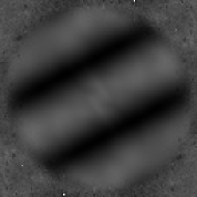
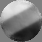
Figure 1: Modulus (left) and bispectrum-phase (right) of the complex visibility for Gliese~866. They have been computed from speckle-interferometric data obtained on 27 September 1996 at the 3.5 m-telescope on Calar Alto in the K-band using the NIR array camera MAGIC. The bispectrum-phase has only been calculated inside a circle that corresponds to the Nyquist spatial frequency which is $7.0\,\mathrm{arcsec}^{-1}$ for the adopted pixel scale.

To obtain a highly precise relative astrometry which is crucial for orbit determination one has to provide a good calibration of pixel scale and detector orientation. For the speckle observations since 9 July 1995 this calibration has been done using astrometric fits to images of the Trapezium cluster, where precise astrometry has been given by McCaughrean & Stauffer (McCaughrean94 (1994)). During the previous observing runs binary stars with well known orbits were observed for calibrating pixel scale and detector orientation. By doing subsequent observations of these systems and calibrating them with the Trapezium cluster we have put all speckle observations since July 1993 in a consistent system of pixel scale and detector orientation.

3 Results

Figure 2: Improved relative orbit of Gliese~866 AB (solid) compared to the orbit derived by L90 (dotted). North is up and east is to the left. The individual measurements are connected to the predicted positions by lines. For the two measurements represented by open circles only one coordinate could be derived from the observation, the other one is taken from the predicted orbit. The triangle denotes the HST measurement (No. 16 in Table 1). The periastron is indicated by a vertical bar. The line of nodes also is plotted.

After combining the relative astrometry from L90 and our new observations, there are now 37 independent data points for the orbital motion of the visual pair in Gliese~866. They are plotted in Fig. 2, together with the result of an orbital fit that used the method of Thiele and van den Bos, including iterative differential corrections (Heintz Heintz78 (1978)).

Table 2: Orbital elements for Gliese 866

Orbital element	Result
Node	$\Omega=162.1^{\circ}\pm 0.4^{\circ}$
Longitude of periastron	$\omega=-17.7^{\circ}\pm 1.1^{\circ}$
Inclination	$i=112.4^{\circ}\pm 0.5^{\circ}$
Semi majoraxis	$A=(0.346\pm 0.004)\,\mathrm{arcsec}$
Period	$P=(2.2506\pm 0.0033)\,\mathrm{yr}$
Eccentricity	$e=0.437\pm 0.007$
Periastron time	$t_{P}=1987.236\pm 0.014$

The orbital elements resulting from a fit to the full data set are given in Table 2. Since we don’t know which node is ascending and which one is descending, we choose – as usually is done – $\Omega$ to be between $0\degr$ and $180\degr$. $\omega$ is the angle between the adopted $\Omega$ and the periastron (positive in the direction of motion), and $i>90\degr$ means clockwise motion.
Gliese~866 has a trigonometric parallax $\pi=289.5\pm 4.4\,\mathrm{mas}$ (van Altena et al. vanAltena95 (1995)). In the following calculations we use the external error of the parallax: $6.8\,\mathrm{mas}$ instead of the (internal) value given by van Altena et al. This yields a distance of $3.45\pm 0.08\,\mathrm{pc}$, a semi majoraxis of $1.19\,\mathrm{AU}$ and finally – using Kepler’s third law – a system mass $M_{\mathrm{Sys}}=0.336\pm 0.026\,M_{\odot}$. This result remains unchanged within the uncertainties if the calculation is done with natural subsets of the data (see Table 3). There is particularly no significant difference if only the 2D data points with good astrometric calibration (see Sect. 2) are used. Because it covers the longest time span, we take the result for the full data set as best values for orbit and system mass.

Table 3: Derived system mass for different subsets of the data

Data set	N	$M_{\mathrm{Sys}}/M_{\odot}$
all data	37	0.336 $\pm$ 0.026
only our speckle data	28	0.336 $\pm$ 0.032
only our 2D speckle data with	13	0.340 $\pm$ 0.035
direct astrometric calibration

4 Discussion

Most of the uncertainty in system mass is from the parallax error. Further improvements in determining this parameter will improve the accuracy of system mass considerably beyond the present $\pm 7.5\,\%$.
We also want to get a first estimate of the components’ masses in order to judge the probability for a substellar object in the system. This cannot be done empirically from our data, because there are no published radial velocities for Gliese~866. Instead we use the mass-luminosity relation given by Henry & McCarthy (Henry93 (1993)) as

$$\log\frac{M}{M_{\odot}}\pm 0.067=-0.1668M_{\mathrm{K}}+0.5395$$ (1)

for absolute K magnitudes $9.81\leq M_{\mathrm{K}}<7.70$.
This approach is only valid if there is no large shift between the spectral energy distributions of the components. To check this we consider the observations taken at other wavelengths. At $917\,\mathrm{nm}$ the flux ratio is comparable to that in the K-band and also to the flux ratios in other NIR filters given by L90 (Table 3 therein). This supports the conclusion of L90 that both (visual) components nearly have the same spectral type and effective temperature. At $845\,\mathrm{nm}$ L90 have measured a higher flux ratio of $I_{\mathrm{B}}/I_{\mathrm{Aa}}=0.83\pm 0.1$, but this wavelength lies at the edge of a strong TiO absorption feature (L90, Fig. 8 therein), so an extrapolation of flux ratios into the visible is not straightforward. Furthermore Henry et al. (Henry99 (1999)) have observed Gliese~866 with the F583W filter of the HST. The resultant flux ratio in V is $I_{\mathrm{B}}/I_{\mathrm{Aa}}=0.69\pm 0.06$ and thus again close to the values in the near infrared. The fact that the flux ratio $I_{\mathrm{B}}/I_{\mathrm{Aa}}$ is nearly constant over a large range of wavelengths indicates that all three components of the Gliese~866 system have similar effective temperatures and thus similar masses. This idea is further supported by the combined spectrum of Gliese~866 (L90, Fig. 8 therein) that shows the deep molecular absorptions of an M5.5 star.
The apparent magnitude of the system is $K=(5.56\pm 0.02)\,\mathrm{mag}$ (Leggett Leggett92 (1992) and references therein). Combined with the distance given above the absolute system magnitude is $(7.87\pm 0.04)\,\mathrm{mag}$. The K-band flux ratios given in Table 1 result in a mean value of $I_{\mathrm{B}}/I_{\mathrm{Aa}}=0.57\pm 0.01$. We take the components of the spectroscopic pair Gliese~866 Aa to be equally bright. Because we have only given qualitative arguments for this assumption, we use an error reflecting this uncertainty: $I_{\mathrm{a}}/I_{\mathrm{A}}=1.0\pm 0.5$. This yields the components’ absolute K magnitudes:

$$M_{\mathrm{K}}(A) = M_{\mathrm{K}}(a)=(9.11\pm 0.32)\,\mathrm{mag}$$

$$M_{\mathrm{K}}(B) = (8.98\pm 0.05)\,\mathrm{mag}$$ (2)

The resulting masses from Eq. 1 then are:

$$M_{\mathrm{A}} = M_{\mathrm{a}}=(0.105\pm 0.021)M_{\odot}$$

$$M_{\mathrm{B}} = (0.110\pm 0.018)M_{\odot}.$$ (3)

The given uncertainties originate from the error of the K magnitudes (Eq. 2) and the error of the mass-luminosity relation itself (Eq. 1). The sum of these masses is $M_{\mathrm{Sys}}=0.320\pm 0.035\,M_{\odot}$ and is thus within the uncertainties consistent with the dynamical system mass $M_{\mathrm{Sys,dyn}}=0.336\pm 0.026\,M_{\odot}$ derived above.

5 Summary

From a new determination of the visual orbit we have given an improved determination of the system mass in Gliese~866. With simplifying assumptions we have given estimates for the components’ masses using the mass-luminosity relation by Henry & McCarthy (Henry93 (1993)). The sum of the components’ masses estimated in this way is consistent with the dynamically obtained system mass. We conclude that there is no substellar object in the triple system Gliese~866 despite the fact that the total system mass is only $0.34\,M_{\odot}$.

- (1) Delfosse X., Forveille T., Beuzit J.L., et al. , 1999, A&A 344, 897
- (2) Heintz W.D., 1978, ”Double Stars”, D. Reidel Publishing Company, Dordrecht
- (3) Henry T.J., McCarthy D.W., 1993, AJ 106, 773
- (4) Henry T.J., Franz O.G., Wasserman L.H., et al. , 1999, ApJ 512, 864
- (5) Knox K.T., Thompson B.J., 1974, ApJ 193, L45
- (6) Leggett S.K., 1992, ApJS 82, 351
- (7) Leinert Ch., Haas M., 1989, A&A 221, 110
- (8) Leinert Ch., Jahreiß H., Haas M., 1986, A&A 164, L29
- (9) Leinert Ch., Haas M., Allard F., et al. , 1990, A&A 236, 399 (L90)
- (10) Lohmann A.W., Weigelt G., Wirnitzer B., 1983, Applied Optics 22, 4028
- (11) McCarthy D.W., Cobb M.L., Probst R.G., 1987, AJ 93, 1535
- (12) McCaughrean M.J., Stauffer J.R., 1994, AJ 108, 1382
- (13) Oppenheimer B.R., Kulkarni S.R., Stauffer J.R., 2000, in Protostars and Planets IV, ed. V. Mannings, A.P. Boss, S.S. Russell (Tucson: University of Arizona), in press
- (14) van Altena W.F., Lee J.T., Hoffleit E.D., 1995, The General Catalogoue of Trigonometric Stellar Parallaxes, Fourth Edition, Yale University Observatory