Soft X-ray AGN Luminosity Function from ROSAT Surveys

Abstract

We investigate the evolution of the 0.5-2 keV soft X-ray luminosity function (SXLF) of active galactic nuclei (AGN) using results from ROSAT surveys of various depth. The large dynamic range of the combined sample, from shallow large-area ROSAT All-Sky Survey (RASS)-based samples to the deepest pointed observation on the Lockman Hole, enabled us to trace the behavior of the SXLF. The combined sample includes about 690 AGNs. As previously found, the SXLF evolves rapidly as a function of redshift up to $z\sim 1.5$ and is consistent with remaining constant beyond this redshift.

We have tried to find a simple analytical description of the SXLF in the overall redshift and luminosity range, using Maximum-Likelihood fits and Kolgomorov-Smirnov tests. We found that a form of the Luminosity-Dependent Density Evolution (LDDE), rather than the classical Pure Luminosity Evolution (PLE) or the Pure Density Evolution (PDE) models, gives an excellent fit to the data. Extrapolating one form of the LDDE model (LDDE1) explains $\approx 60\%$ of the estimated soft extragalactic Cosmic X-ray Background (CXRB). We have also found another representation (LDDE2), which produces $\approx 90\%$ of the CXRB and still gives an excellent fit to the sample AGNs. These two versions of the LDDE models can be considered two extremes of the possible extrapolations of the SXLF below the flux limit of the survey.

We have also investigated the evolution of the number density of luminous QSOs with ${\rm Log}\,L_{\rm x}>44.5$ $[h_{\rm 50}{\rm erg\,s^{-1}}]$, where the evolution can be traced up to the high redshift. We have compared the results with similar quantities in optically- and radio-selected luminous QSOs. Unlike these QSOs, evolution of the ROSAT-selected QSOs do not show evidence for the decrease of the number density in $z\ga 3$. The statistical significance of the difference is, however, marginal.

1 Introduction

The AGN/QSO luminosity function and its evolution with cosmic time are key observational quantities on understanding the origin of and accretion history onto supermassive balckholes, which are now believed to occupy the centers of most galaxies. Since X-ray emission is one of the prominent characters of the AGN activity, X-ray surveys are effective means of sampling AGNs for the luminosity function and evolution studies. The Röntgen satellite (ROSAT), with its unprecedented imaging capabilities, provided us with soft X-ray surveys with various depths, ranging from the ROSAT All-Sky Survey (RASS) to the ROSAT Deep Survey (RDS) on the Lockman Hole (Hasinger et al. rds1 (1998)). Various optical identification programs of the survey fields have been conducted and the combination of these now enabled us to construct the soft X-ray luminosity function (SXLF) as a function of redshift.

The evolution of SXLF has already been seen in the Extended Medium Sensitivity Survey (EMSS) AGNs (Maccacaro et al. emss1 (1991); Della Ceca et al. emss2 (1992)) for high-luminosity AGNs. Combining results from deep ROSAT PSPC surveys and the EMSS has extended the sample into the higher-redshift lower-luminosity regime, providing much wider baseline to explore the evolution properties (e.g. Boyle et al. 1994; Jones et al. 1996; Page et al. 1996). All of these were characterized by a pure luminosity evolution model (PLE) with approximately $\propto(1+z)^{3}$ up to $z\approx 2$, and consistent with no evolution beyond that point. Using a larger ROSAT sample, Page et al. (1997) found that PLE underpredicts the number of high-redhsift low luminosity AGNs for $q_{0}=0.5$. Simple extrapolations of any of the PLE expressions only explain $\sim 30-50\%$ of the soft X-ray Background (0.5-2 keV) by AGN.

Because of the relatively large PSF of the ROSAT PSPC, the identifications of the deepest ROSAT PSPC surveys are sometimes ambiguous and misidentifications can occur. Based on results of the optical followup studies of ROSAT PSPC surveys, a number of groups, including the Deep ROSAT Survey (DRS; Griffiths et al. gri96 (1996)) and UK Deep Survey (UKD; McHardy et al. ukd (1998)) report a population of X-ray sources called “Narrow Emission-line Galaxies” (NELG) at faint fluxes. On the other hand, faint X-ray sources found in the ROSAT Deep Survey on the Lockman Hole (RDS-LH), which have accurate source positions from 1 million seconds of ROSAT HRI data, are still predominantly AGNs down to the faintest fluxe in the survey (Schmidt et al. rds2 (1998); Hasinger et al. has99 (1999)). Some of these have optical spectra which apparently show only narrow-lines but have other signs of an AGN activity and might have been classified as “NELGs” at the criteria of other groups. On the other hand, Lehmann et al. (1999b ) have compared redshift distributions of the RDS X-ray AGNs, UKD X-ray sources, non X-ray emitting (at the RDS-LH limit) field galaxies showing narrow emission-lines. They found that the redshift distribution of UKD X-ray sources has a significant excess over that of the RDS-LH sources at $z<0.4$. This excess was dominated by “NELGs”, whose redshift distribution was similar to that of non X-ray source narrow emission-line field galaxies. This shows that a significant fraction of “NELGs” are likely to be misidentifications by chance coincidences. This observation seems to contradict with estimations of the relatively low probabilities of such chance coincidences by the DRS and UKD groups. A more detailed comparison is urgently needed. Misidentifications affect SXLF estimates in two ways, i.e., by putting a wrong object into the sample and by missing the true identifications. Thus it is important to have a high spatial resolution image to obtain unambiguous identifications, especially in the faintest regime.

In this study, we investigate the global behavior of the soft X-ray luminosity function (SXLF) of AGNs from a combined sample of various ROSAT surveys. We use the term “AGN” for both Seyfert galaxies, including type 1’s and type 2’s, and QSOs. Preliminary work, using earlier versions of the combined sample, have been reported in Hasinger (has_xs (1998)) and Miyaji et al. (1999a ) (hereafter M99a), while in this work, we have made a more extensive analysis with updated ROSAT Bright Survey (RBS) and ROSAT Deep Survey (RDS) catalogs including new identifcations from observations made in the winter-spring season of 1999. In this paper, we put emphasis on the expressions representing the global behavior of the SXLF. Presenting separate expressions in several redshift intervals, giving more accurate representation of the data in the redshift ranges of interest will be a topic of a future paper (Miyaji et al. in preparation, paper II). In paper II, we will also present tables of full numerical values of the binned SXLF.

We use a Hubble constant $H_{0}=50\,h_{50}\,$ $[{\rm km\,s^{-1}\,Mpc^{-1}}]$. The $h_{50}$ dependences are explicitly stated. We calculate the results with common sets of cosmological parameters: $(\Omega_{\rm m},\Omega_{\Lambda})=$(1.0,0.0) and (0.3,0.0). For some important parameterized expressions, we also show the results for $(\Omega_{\rm m},\Omega_{\Lambda})=$ (0.3,0.7).

2 The ROSAT Surveys used in the analysis

We have used soft X-ray sources identified with AGNs with redshift information from a combination of ROSAT surveys in various depths/areas from a number of already published and unpublished sources. In order to avoid the possible bias from the large-scale overdensity and the distortion of the redshift-distance relation based on bulk-flows in the nearby universe (e.g. Tully & Shaya tusha (1984)), we have excluded objects within $z<0.015$ from the analysis.

The surveys we have used are summarized in Table  1. Two optical followup programs from the ROSAT All-Sky Survey (RASS) (Voges rass (1994)), a serendipitous survey of the ROSAT PSPC pointed observations (RIXOS), and a number of deep pointings specifically aimed for deep surveys. Here we describe the AGN sample from each survey.

All surveys, except for a part of the the Lockman Hole, are based on the ROSAT PSPC count rates in the pulse-invariant (PI) channel range corresponding to 0.5 - 2 keV. For most sources in the Lockman Hole, we have used the deeper HRI count rates (see below) with no spectral resolution and sensitive to the 0.1 - 2 keV.

In order to convert the countrate to flux, we have to assume a spectrum. Hasinger et al. (has93 (1993)) obtained the value of $\Gamma=1.96\pm.11$ for the average spectral photon index in the Lockman Hole. Other works (Romero-Colenero et al. rom (1996); Almaini et al. alm (1996)) also found similar spectral index for AGNs, but a harder index $\Gamma\approx 1.5$ for the “NELGs”. The same class as a part of the population they have classified as NELGs may fall into our sample. In any case, the ROSAT countrate to the unabsorbed 0.5-2 keV flux conversion has been made assuming a power-law with a photon index of $\Gamma=2.0$ and corrected for the Galactic absorption. In effect, the Galactic column density changes the response curves for the flux-to-countrate conversion. However, the extragalactic surveys are mainly concentrated on the part of the sky where the Galactic absorption is low. Typical values are $(0.5-1)\times 10^{20}$ ${\rm[cm^{-2}]}$ for the deep surveys and a maximum of $16\times 10^{20}$ ${\rm[cm^{-2}]}$ for a small portion of the sky covered by the RBS. Within this range, the conversion between the $S_{\rm x}$ (here and hereafter, $S_{\rm x}$ represents the 0.5-2 keV flux and $S_{\rm x14}$ is the same quantity measured in units of $10^{-14}[{\rm erg\,s^{-1}\,cm^{-2}}]$) the ROSAT PSPC countrate (in the corresponding channel range) only weakly dependent on the spectral shape and varies by about $\pm 3$% for spectral indices $\Gamma=2.0\pm 0.7$. We discuss the conversion for the HRI case in Sect. 2.7.

For the computation of the SXLF, it is important to define the available survey area as a function of limiting flux. In case there is incompleteness in the spectroscopic identifications, we have made the usual assumption that the redshift/classification distribution of these unidentified sources is the same as the identified sources at similar fluxes. This can be attained by defining the ’effective’ survey area as the geometrical survey area multiplied by the completeness of the identifications. This assumption is not correct when the source is unidentified due to non-random causes, e.g., no prominent emission lines in the observed spectrum. However, given the high completeness of the samples used in our analysis, this does not affect the results significantly, except for the faintest end of RDS-LH. We discuss the effects of the incompleteness at this faint end in Sect. 3.5.

Below we summarize our sample selection and completeness for each survey.

Table 1: ROSAT Surveys used in the Analysis

Surveya	$S^{\rm lim}_{\rm x14}$	Area	No. ofb
	$[{\rm erg\,s^{-1}\,cm^{-2}}]$	$[{\rm deg}^{2}]$	AGNs
RBS	$\approx 250$	$2.0\times 10^{4}$	216
SA-N	$\approx 13$	$685.$	130
RIXOS	$3.0$	$15.$	205
NEP	$1.0$	$0.21$	13
UKD	$0.5$	$0.16$	29
RDS-Marano	$0.5$	$0.20$	30
RDS-LH	$0.17-0.9$	$0.30$	68

^a Abbreviations – RBS: The ROSAT Bright Survey, SA-N: The Selected Area-North, RIXOS: The ROSAT International X-ray Optical Survey, NEP: The North Ecliptic Pole UKD: The UK Deep Survey, RDS-Marano: The ROSAT Deep Survey – Marano field, RDS-LH: The ROSAT Deep Survey – Lockman Hole. See text for references. ^b Excluding AGNs with $z<0.015$.

Figure 1: The survey area of the combined sample are plotted as a function of the limiting 0.5-2 keV flux limit (solid line). For reference, $[N(>S)]^{-1}$ for all the X-ray sources is overplotted (dashed-line).

2.1 The ROSAT Bright Survey (RBS)

The RBS program aims for a complete identification of the $\sim$ 2000 brightest sources in the ROSAT All-Sky Survey (RASS) for $|b|>30\deg$ (Fischer et al. rbs0 (1998); Schwope et al. in preparation ) measured in the entire ROSAT band (0.1-2.4 keV). For our purposes, we have extracted a subset selected by the ROSAT Hard band (0.5-2 keV) countrate of $CR_{\rm hard}\geq 0.2$ $[{\rm cts\;s^{-1}}]$, which makes a complete hard countrate-limited sample. Five sources in this subsample have further been identified as AGNs since M99a and included in the analysis. This subsample now has been completely identified.

Since the absorption in our galaxy varies from place to place, the same countrate limit corresponds to different 0.5-2 keV flux limits based on different galactic $N_{\rm H}$ values. The $N_{\rm H}$ value range from $(0.5-16)\times 10^{20}$ $[{\rm cm}^{-2}]$.

2.2 The RASS Selected-Area Survey – North

This survey uses several high galactic latitude areas of RASS (a total of $685{\rm[deg^{2}]}$) for optical identification of the sources down to about an order of magnitude fainter than the RBS. The fields selected for the survey have the Galactic column ranging $N_{\rm H}=(2-11)\times 10^{20}$ $[{\rm cm}^{-2}]$. Details of the survey have been described in Zickgraf et al. (zick97 (1997)) and the catalog of source identifications has been published by Appenzeller et al. (app98 (1998)). We have further selected our sample such that each field has a complete ROSAT hard-band (0.5-2 [keV]) countrate-limited sample with complete identifications ($CR_{\rm hard}>$ 0.01-0.05 $[{\rm cts\;s^{-1}}]$).

2.3 The RIXOS Survey

The ROSAT International X-ray Optical Survey (RIXOS), Mason et al. (rixos (1999)) (see also Page et al. page96 (1996)) is a serendipitous survey of $\approx 80$ PSPC fields covering 15 deg² of the sky. The flux limit of the deepest field is $S_{\rm x14}=3.0$, while the actual completeness limit varies from field to field. The identification is $97\%$ complete, thus the effect of the identification incompleteness is negligible considering statistical errors.

2.4 The North Ecliptic Pole (NEP) Survey

The data are from Bower et al. (nep (1996)), which gave a catalog of 20 sources in the 15$\aas@@fstack{\prime}$5 radius region with $S_{\rm x14}\geq 1.0$. One object, RX J1802.1+6629 did not have a redshift entry in Table 2 of Bower et al., but in the text, they argued that the most probable interpretation of this object was a weak-lined QSO at $z\sim 1$. Thus we have assigned a redshift of 1.0 to this source. There is one unidentified source, making the identificaton of the sample 95% complete. Thus we have set the effective survey area of the NEP survey as 95% of the geometrical area.

2.5 The UK Deep Survey

Based on a 115 [ks] of ROSAT PSPC observation, McHardy et al. (1998) published a list of sources and identification of X-ray sources down to $S_{\rm x14}=0.19$. A significant fraction of their identifications are “NELGs” (Narrow Emission-Line Galaxies) and the fraction increases towards fainter fluxes. As mentioned in Sect. 1, a part of these NELGs are likely to be misidentifications. The identifications of other NELGs might be correct, but those would have been classified as AGNs with the criteria of Schmidt et al. (rds2 (1998)).

To include the results of the UKD survey in our sample, we would like to include their NELGs in the latter category, but exclude those in the former category. We find that the redshift distribution of the AGN+NELG classes in the UKD survey is significantly different from the AGN+galaxy classes in the Lockman survey if we include all sources down to $S_{\rm x14}\geq 0.19$. If we limit the sample to brighter sources ($S_{\rm x14}\geq 0.5$), the redshift distributions are consistent with each other. Thus, in this work, we limit the samples from UKD and other deep PSPC surveys to $S_{\rm x14}\geq 0.5$, assuming that the misidentification problem would not affect the analysis significantly above this limit.

2.6 The ROSAT Deep Survey – Marano Field

For the same reason as the UKD case, we have also used the same flux cutoff $S_{\rm x14}\geq 0.5$ for the survey in the 15$\arcmin$- radius region on the Marano field (Zamorani et al. marano (1999)), based on a deep PSPC exposure. Source fluxes of their catalog have been updated since the version used by M99a. The identifications are 100% complete for the 14 sources in $S_{\rm x14}\geq 1$ and 4 of the 27 sources remain unidentified or ambiguous (85% complete) in $0.5\leq S_{\rm x14}<1$. As before, we have reduced the survey area by 15% in this flux range to define the effective survey area used in the SXLF calculations.

2.7 The ROSAT Deep Survey – Lockman Hole

There are 200 ks of PSPC and 1 Msec of HRI observations on this field (Hasinger et al. rds1 (1998)). The source list and identifications for the brightest 50 sources ($S_{\rm x14}>0.5$) have been published (Schmidt et al. rds2 (1998)). In this work, we have included further unpublished identifications down to $S_{\rm x14}=0.17$. These include identifications and redshifts based on spectra obtained in March 1998 with the Keck 10m telescope (Hasinger et al. has99 (1999)), which have also been included in M99a. Further four spectroscopic identifications obtained with the Keck telescope in February 1999 have been added to the sample since M99a.

The conversion between the HRI countrate and the 0.5-2 keV flux has been determined from the mean values of overlapping sources between the HRI and PSPC. The convsersion carries more uncertainties based on spectra, because the HRI has practically no spectral resolution and has some sensitivity down to 0.1 keV. With the HRI, the conversion factor varies by $\pm 40\%$ for photon indices $\Gamma=2.0\pm 0.7$.

The basic strategy of defining the combined PSPC-HRI sample has been explained in Hasinger et al. (has99 (1999)). In this paper, we have slightly modified the flux-limit and areas of the HRI sample in order to optimize our AGN sample in the presence of new identifications:

• We use the deeper HRI-detected sample and HRI fluxes for the region 12.0 arcminutes from the HRI center (0.126 deg²). At the faintest fluxes ($0.17\leq S_{\rm x14}<0.24$), we have further limited the area to 10.1 arcminutes from the HRI center (0.090 deg²). This choice allows us to avoid the problem of incomplete source detection due to source confusion (see Fig. 2b of Hasinger et al. has99 (1999)). A total of 48 AGNs are present in this HRI sample.

• Outside of the HRI region defined above, and within 18.4 arcminutes from the PSPC center, we have used the PSPC detected sources and PSPC fluxes. This corresponds to 0.175 deg². For completeness, we have imposed a flux cutoff of $S_{\rm x14}\geq 0.38$ for PSPC off-axis angles smaller than 12$\arcmin$.5 and $S_{\rm x14}\geq 0.97$ for PSPC offaxis angles between 12.5 and 18.4 arcminutes respectively.

• The sources in the HRI/PSPC combined sample have been 100% identified for $S_{\rm x14}\geq 0.38$. Four of the 31 sources in $0.17\leq S_{\rm x14}<0.38$ remain spectroscopically unidentified. Thus we have reduced the effective survey area by 13% for $0.17\leq S_{\rm x14}<0.38$ to compensate for the identification incompleteness.

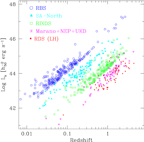
Figure 2: The AGNs in the combined sample are plotted in the $z-LogL_{\rm x}$ for ($\Omega,\Omega_{\Lambda}$) =(1.0,0.0). Different symbols correspond to different surveys as labeled.

2.8 The combined sample

In our combined sample, there are 691 AGNs ranging from $4.2\times 10^{-11}$ to $1.7\times 10^{-15}[{\rm erg\,s^{-1}\,cm^{-2}}]$. The effective survey area for the combined sample is plotted as a function of the limiting flux in Fig. 1, overlaid with the value of $N(>S)^{-1}$, showing that the combined sample indeed covers the above flux range continuously.

The redshift - luminosity scatter digrams of the sample objects are shown in Fig. 2 for the $(\Omega_{\rm 0},\Omega_{\rm\Lambda})=(1.0,0.0)$ universe. In any case, the luminosities have been calculated by:

$$L_{\rm x}=4\pi d_{\rm L}(z)^{2}S_{\rm 0.5-2keV}$$ (1)

where $d_{\rm L}(z)$ is the luminosity distance as a function of redshift, which depends on the choice of cosmological parameters. This corresponds to the no K-correction case. Explanation on our K-correction policy is explained in Sect. 3.1. Hereafter, the symbol $L_{\rm x}$ refers to the quantity defined in Eq. (1) expressed in units of $h_{50}^{-2}{\rm[erg\,s^{-1}]}$, unless otherwise noted.

3 The ROSAT AGN SXLF

3.1 K-Correction and AGN subclasses

In this section, we choose to present the SXLF in the observed 0.5-2 keV band, i.e., in the $0.5(1+z)-2(1+z)$ keV range in the object’s rest frame. Thus no K-correction has been appplied for our expressions presented in this section. Also we choose to include all emission-line AGNs (i.e., except BL-Lacs), including type 1’s and type 2’s. The primary reason for these choice is to separate the model-independent quantities, directly derived from ROSAT surveys, from model-dependent assumptions. Here we explain the philosophy behind these choices in detail.

There are a variety of AGN spectra in the X-ray regime, but the information on exact content of AGNs in various spectral classes is very limited. Currently popular models explaining the origin of the 1-100 keV CXRB involve large contribution of self-absorbed AGNs (Madau et al.madau94 (1994); Comastri et al. coma95 (1995); Miyaji et al. 1999b ; Gilli et al. gilli99 (1999)). Although they are selected against in the ROSAT band, some of these absorbed AGNs come into our sample. These absorbed AGNs certainly have different K-correction properties than the unabsorbed ones. While these absorbed AGNs are mainly associated with those optically classified as type 2 AGNs, the correspondence between the optical classification and the X-ray absorption is not straightforward. Especially, there are many optically type-1 AGNs (with broad-permitted emission lines), which show apparent X-ray absorption of some kind. For example, a number of Broad Absorption Line (BAL) QSOs are known to have strongly absorbed X-ray spectra (e.g. Mathur et al. phl5200 (1995); Gallagher et al. gallag (1999)). At the fainter/high-redshift end of our survey, there may be some broad-line QSOs of this kind or some intermediate class. Broad-line AGNs with hard X-ray spectra have been found in a number of hard surveys (Fiore et al. fiore (1999); Akiyama et al. aki (1999)). In Schartel et al. (schar97 (1997))’s study, all except two of the 29 AGNs from the Piccinotti et al.’s (picci (1982)) catalog have been classified as type 1’s, but about a half of them show X-ray absorption, some of which might be caused by warm absorbers. In view of these, using only optically-type 1 AGNs to exclude self-absorbed AGNs is not appropriate. Also optical classification of type 1 and type 2 AGNs depend strongly on quality of optical spectra. Thus classification may be biased, e.g. as a function of flux. However, the SXLF for the type 1 AGNs is of historical interest and shown in Appendix A. As shown in Appendix A., non type-1 AGNs are very small fraction of the total sample and excluding these does not change the main results significantly.

On the other hand, our sample of 691 AGNs with extremely high degree of completeness carries little uncertainties in the fluxes in the 0.5-2 keV band in the observer’s frame, redshifts, and classification as AGNs. Thus, we choose to show the SXLF expression in the observed 0.5-2 keV band, or 0.5(1+z)-2(1+z) keV band at the source rest frame, in order to take full advantage of this excellent-quality sample without involving major sources of uncertainties. The expressions in the observed band may have less direct relevance for discussion on the actual AGN SXLF evolution. However they are more useful for discussing the contribution of AGNs to the Soft X-ray Background (Sect. 4), interpretation of the fluctuation of the soft CXRB, and evaluating the selection function for studying clustering properties of soft X-ray selected sample AGNs.

In practice, the expressions can also be considered a K-corrected SXLF at the zero-th approximation, since applying no K-correction is equivalent to a K-correction assuming $\Gamma=2$. This index has been historically used in previous works (e.g. Maccacaro et al. emss1 (1991); Jones et al. jones96 (1996)), thus our expression is useful for comparisons with previous results. A $\Gamma=2$ power-law spectrum can be considered the best-bet single spectrum characterizing the sample, because in the ROSAT sample, absorbed AGNs (including type 2 AGNs, type 1 Seyferts with warm absorbers, BAL QSOs) are highly selected against. Nearby type 1 AGNs show an underlying power-law index of $\Gamma=2$ at $E\ga 1$[keV] (e.g. George et al. george (1998)), which is the energy range corresponding to 0.5-2 keV for the high redshifts where K-correction becomes important. The reflection component, which makes the spectrum apparently harder, becomes important only above 10 keV. This is outside of the ROSAT band even at $z\ga 4$. The above argument is consistent with the fact that the average spectra of the faintest X-ray sources, especially those indentified with broad-line AGNs, have $\Gamma\approx 2$ (Hasinger et al. has93 (1993); Romero-Colmenero et al. rom (1996); Almaini et al. alm (1996)) in the ROSAT band. Therefore, at the zero-th approximation, one can view our expression as a K-corrected SXLF of AGNs, especially at high luminosities. The goodness of this approximation is highly model-dependent and a discussion on further modeling beyond this zero-th approximation is given in Sect. 6.

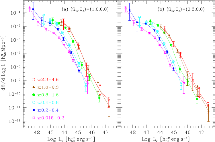
Figure 3: The $\Sigma V_{\rm a}^{-1}$ estimates of the SXLFs are plotted with estimated 1$\sigma$ errors. Different symbols correspond to different redshift bins as indicated in the panel (a) and data points belonging to the same redshift bin are connected. The position of the symbol attached to a downward arrow indicates the 90% upper limit (corresponding to 2.3 objects), where there is no AGN detected in the bin.

3.2 The binned SXLF of AGNs

The SXLF is the number density of soft X-ray-selected AGNs per unit comoving volume per ${\rm Log}\;L_{\rm x}$ as a function of $L_{\rm x}$ and $z$. We write the SXLF as:

$$\frac{{\rm d}\Phi}{{\rm d\;Log}\;L_{\rm x}}({\rm Log}\;L_{\rm x},z).$$

Fig.3 shows the binned SXLF in different redshift shells estimated using the $\sum 1/V_{\rm a}$ estimator:

$$\frac{{\rm d}\;\Phi}{{\rm d\;Log}\;L_{\rm x}}(\overline{{\rm\;Log}\;L_{{\rm x}j}},\overline{z_{j}})\approx\frac{\sum_{i}\;V_{\rm a}^{j}(L_{{\rm x}i})^{-1}}{(\Delta\;{\rm Log}\;L_{\rm x})_{j}},$$ (2)

where the $L_{\rm x}-z$ bins are indexed by $j$ and AGNs in the sample falling into the $j$-th bin are indexed by $i$, $V_{\rm a}^{j}(L_{{\rm x}})$ is the available comoving volume in the redshift range of the $j-th$ bin where an AGN with luminosity $L_{\rm x}$ would be in the sample. The luminosity function is estimated at ($\overline{{\rm Log}\;L_{{\rm x}}}_{j}$,$\overline{z_{j}}$), where a bar represents the $V_{\rm a}^{-1}$ weighted average over the AGNs falling into the $j$-th bin. Also $(\Delta\;{\rm Log}\;L_{\rm x})_{j}$ is the size of the $j-$th bin in ${\rm Log}\;L_{\rm x}$.

Rough 1$\sigma$ errors have been estimated by:

$$\sigma{\left[\frac{{\rm d}\;\Phi}{{\rm d\;Log}\;L_{\rm x}}(\overline{{\rm Log}\;L_{\rm x}}_{j},\overline{z_{j}})\right]}\approx\frac{\sqrt{\sum_{i}\;V_{\rm a}(L_{{\rm x}i})^{-2}}}{(\Delta\;{\rm Log}\;L_{\rm x})_{j}}.$$ (3)

In case there is only one AGN in the bin, we have plotted error bars which correspond to the exact Poisson errors corresponding to the confidence range of Gaussian 1$\sigma$. In this way, we can also avoid infinitely extending error bars in the logarithmic plot.

Fig. 3(a)(b) shows the binned SXLF calculated for $(\Omega_{\rm m},\Omega_{\rm\Lambda})=(1.0,0.0)$ and $(0.3,0.0)$ respectively. In Fig. 3, we have also plotted some interesting upper-limits, in case there is no object in the bin. In the figure, we show upper limits corresponding to 2.3 objects (90% upper-limit). See caption for details.

We note that the binned $\sum 1/V_{\rm a}$ estimate can cause a significant bias, especially because the size of the bins tend to be large. For example, at low luminosity bins with corresponding fluxes close to the survey limit, the value of $V_{\rm a}$ can vary by a large factor within one bin. Also the choice of the point in $L_{\rm x}$ space representative of the bin, at which the SXLF values are plotted, may change the impression of the plot significantly. Thus the SXLF estimates based on the binned $\sum 1/V_{\rm a}$ can be used to obtain a rough overview of the behavior, but should not be used for statistical tests or a comparison with models. Full numerical values of the binned SXLF including $\sum 1/V_{\rm a}$ values, improved estimations by a method similar to that discussed by Page & Carrera page99 (1999), and the numbers of AGNs in each bin will be presented in paper II.

A number of features can be seen in the SXLF. As found previously, our SXLF at low $z$ is not consistent with a single power-law, but turns over at around ${\rm Log}\;L_{\rm x}\sim 43-44$. The SXLF drops rapidly with luminosity beyond the break. We see a strong evolution of the SXLF up to the $0.8\leq z<1.6$ bin, but the SXLF does not seem to show significant evolution between the two highest redshift bins. Figs. 3 (a)(b) show that these basic tendencies hold for the two extreme sets of cosmological parameters.

3.3 Analytical expression – statistical method

It is often convenient to express the SXLF and its evolution in terms of a simple analytical formula, in particular, when using as basic starting point of further theoretical models.

Here we explain the statistical methods of parameter estimations and evaluating the acceptance of the models. A minimum $\chi^{2}$ fitting to the binned $1/V_{\rm a}$ estimate is not appropriate in this case because it can only be applied to binned datasets with Gaussian errors and at least 20-25 objects per bin are required to achieve this. In our case, such a bin is typically as large as a factor of 10 in $L_{\rm x}$ and a factor of two in $z$, thus the results would change depending where in the $(z\,L_{\rm x})$ bin the comparison model is evaluated.

The Maximum-Likelihood method, where we exploit the full information from each object without binning, is a useful method for parameter estimations (e.g. Marshall et al. mar83 (1983)), while, unlike $\chi^{2}$, it does not give absolute goodness of fit. The absolute goodness of fit can be evaluated using the one-dimensional and two-dimensional Kolgomorov-Smirnov tests (hereafter, 1D-KS and 2D-KS tests respectively; Press et al.numrec (1992); Fasano & Franceschini ff_2dks (1987)) to the best-fit models.

As our maximum-likelihood estimator, we define

$${\cal L}=-2\;\sum_{i}\ln\left[\frac{N({\rm Log}\;L_{{\rm x}i},z_{i})}{\int\int N({\rm Log}\;L_{{\rm x}},z){\rm d\;Log}L_{\rm x}\;{\rm d}z}\right],$$ (4)

where $i$ goes through each AGN in the sample and $N({\rm Log}\;L_{{\rm x}},z)$ is the expected number density of AGNs in the sample per logarithmic luminosity per redshift, calculated from a parameterized analytic model of the SXLF:

$$N({\rm Log}\;L_{{\rm x}},z)=$$

$$\frac{{\rm d}\;\Phi^{\rm model}}{{\rm d\;Log}\;L_{\rm x}}\;d_{\rm A}(z)^{2}\;(1+z)^{3} \;c\,\frac{{\rm d}\tau}{{\rm d}z}(z)\cdot A(L_{\rm x}/d_{\rm L}^{2}),$$ (5)

where $d_{\rm A}(z)$ is the angular distance, $d\tau/dz(z)$ is the differential look back time per unit $z$ (e.g. Boldt boldt87 (1987)) and $A(S_{\rm x})$ is the survey area as a function of limiting X-ray flux (Fig. 1). Minimizing ${\cal L}$ with respect to model parameters gives the best-fit model. Since $\Delta{\cal L}$ from the best-fit point varies as $\Delta\chi^{2}$, we determine the 90% errors of the model parameters corresponding to $\Delta{\cal L}=2.7$. The minimizations have been made using the MINUIT Package from the CERN Program Library (James minuit (1994)).

Since the likelihood function Eq. (4) used normalized number density, the normalization of the model cannot be determined from minimizing ${\cal L}$, but must be determined independently. We have determined the model normalization (expressed by a parameter $A$ in the next subsections) such that the total number of expected objects (the denominator of the right-hand side of Eq. (4)) is equal to the number of AGNs in the sample ($N^{\rm obs}$).

Except for the global normalization $A$, we have made use of the MINUIT command MINOS (see James minuit (1994)) to serach for errors. The command searches for the parameter range corresponding to $\Delta{\cal L}\leq 2.7$, where all other free parameters have been re-fitted to minimize ${\cal L}$ during the search. The estimated 90% confidence error for $A$ is taken to be $1.7A\;(\sqrt{N^{\rm obs}})^{-1}$ and does not include the correlations of errors with other parameters.

The 1D-KS tests have been applied to the sample distributions on the $L_{\rm x}$ and $z$ space respectively. The 2D-KS test has been made to the function $N({\rm Log}\;L_{{\rm x}},z)$. We have shown the probability that the fitted model is correct based on the 1D- and 2D-KS tests. For the 2D-KS test, calculated probability corresponding to the $D$ value from the analytical formula is accurate when there are $\ga 20$ objects and the probabilities $\la 0.2$. If we obtain a probability $\ga 0.2$, the exact value does not have much meaning but implies that the model and data are not significantly different and we can consider the model acceptable. We have searched for models which have acceptance probabilities greater than 20% in all of the KS tests. Strictly speaking, the analytical probability from the KS-test $D$ values are only correct for models given a priori. If we use paramters fitted to the data, this would overestimate the confidence level. A full treatment should be made with large Monte-Carlo simulations (Wisotzki wis (1998)), where each simulated sample is re-fitted and the D-value is calculated. However, making such large simulations just to obtain formally-correct probability of goodness of fit is not worth the required computational task. Instead, we choose to use the analytical probability and set rather strict acceptance criteria.

3.4 Analytical expression – overall AGN SXLF

Using the method described above, we have searched for an analytical expression of the overall SXLF. The overall fit has been made for the redshift range $0.015\leq z<5$. Also for the fits, we have limited the luminosity range to ${\rm Log}\;L_{\rm x}\ga 41.7$.

As described in Sect. 2, the lower redshift cutoff is imposed to avoid effects of local large scale structures, which may cause a deviation from the mean density of the present epoch and thus can cause significant bias to the low luminosity behavior of the SXLF. At the lowest luminosities (${\rm Log}\;L_{\rm x}\leq 41.7$), there is a significant excess of the SXLF from the extrapolation from higher luminosities. This excess connects well with the nearby galaxy SXLF by Schmidt et al. (sbv (1996)) (see also e.g. Hasinger et al. has99 (1999)) and may well contain contamination from star formation activity (see also Lehmann et al. 1999a ). For finding an analytical overall expression, we have not included the AGNs belonging to this regime.

As an analytical expression of the present-day ($z=0$) SXLF, we use the smoothly-connected two power-law form:

$$\frac{{\rm d}\;\Phi\,(L_{\rm x},z=0)}{{\rm d\;Log}\;L_{\rm x}}={A}\;\left[(L_{\rm x}/{L_{*}})^{{\gamma_{1}}}+(L_{\rm x}/{L_{*}})^{{\gamma_{2}}}\right]^{-1}$$ (6)

As a description of evolution laws, the following models have been considered:

3.4.1 Pure-luminosity and pure-density evolutions

As some previous works (e.g. Della Ceca et al. emss2 (1992); Boyle et al. boyle94 (1994); Jones et al. jones96 (1996); Page et al. page96 (1996)), we have first tried to fit the SXLF with a pure-luminosity evolution (PLE) model.

$$\frac{{\rm d}\;\Phi\,(L_{\rm x},z)}{{\rm d\;Log}\;L_{\rm x}}=\frac{{\rm d}\;\Phi\,(L_{\rm x}/e(z),0)}{{\rm d\;Log}\;L_{\rm x}}$$ (7)

Table 2: Best-fit PLE and PDE Parameters

Model	Parametersa/KS probabilities
$(\Omega_{m},\Omega_{\Lambda})$
PLE	$A=(4.0\pm.3)\times 10^{-6}$; $L_{*}=0.33\pm.10$
(1.0,0.0)	$\gamma_{1}=0.60\pm.16$; $\gamma_{2}=2.34\pm.12$; $p1=3.0\pm.2$
	$z_{\rm c}=1.42\pm.17$; $p2=0.3^{+0.5}_{-1.0}$
	$P_{\rm KS}=.002,3\;10^{-5},1\;10^{-5}$ (for $L$,$z$,2D)
PLE	$A=(3.1\pm.2)\times 10^{-6}$; $L_{*}=0.38\pm.12$
(0.3,0.0)	$\gamma_{1}=0.57\pm.16$; $\gamma_{2}=2.35\pm.12$; $p1=2.9\pm.2$
	$z_{\rm c}=1.54\pm.25$; $p2=0.3\pm.7$
	$P_{\rm KS}=.08,.001,2\;10^{-4}$ (for $L$,$z$,2D)
PDE	$A=(6.0\pm.4)\times 10^{-7}$; $L_{*}=1.08\pm.4$
(1.0,0.0)	$\gamma_{1}=0.74\pm.13$; $\gamma_{2}=2.28\pm.11$; $p1=4.6\pm.3$
	$z_{\rm c}=1.60\pm.25$; $p2=0.6\pm 1.1$
	$P_{\rm KS}=0.9,0.9,0.16$ (for $L$,$z$,2D)
PDE	$A=(5.4\pm.3)\times 10^{-7}$; $L_{*}=1.13\pm 0.4$
(0.3,0.0)	$\gamma_{1}=0.76\pm.13$; $\gamma_{2}=2.22\pm.10$; $p1=4.6\pm.3$
	$z_{\rm c}=1.62\pm.26$; $p2=1.3\pm 1.1$
	$P_{\rm KS}={0.8,0.7,0.1}$ (for $L$,$z$,2D)

^aUnits – A: [$h_{50}^{3}\;{\rm Mpc^{-3}}$],   $L_{*}$: [$10^{44}\;h_{50}^{-2}{\rm erg\;s^{-1}}$],   $I_{\rm x12}$: $[10^{-12}{\rm erg\,s^{-1}\,cm^{-2}\,deg^{-2}}]$ in 0.5-2 keV. Parameter errors correspond to the 90% confidence level (see Sect. 3.3).

For the evolution factor, we have used a power-law form:

$$e(z)=\left\{\begin{array}[]{ll}(1+z)^{p1}&(z\leq z_{\rm c})\\ e(z_{\rm c})[(1+z)/(1+z_{\rm c})]^{p2}&(z>z_{\rm c})\\ \end{array}\right..$$ (8)

The best-fit values are listed in the upper part of Table 2 along with 1D-KS and 2D-KS probabilities using the analytical formula. In Table 2 and later tables, the three values of $P_{\rm KS}$ represent the probabilities that the model is acceptable for the 1D-KS test in the $L_{\rm x}$ distribution, 1D-KS test in the $z$ distribution, and 2D-KS test in the ($L_{\rm x}$,$z$) distribution respectively. Note that there are cases which are accepted by 1D-KS tests in both distributions but fail in the 2D-KS test. The results of the fit show that the PLE model is certainly rejected with a 2D-KS probability of $P_{\rm 2DKS}=5\times 10^{-5}$ and $1\times 10^{-2}$ for the $\Omega_{\rm m}$=1 and 0.3 ($\Omega_{\Lambda}=0$) cosmologies respectively.

As an alternative, we have also tried the Pure-Density Evolution model (PDE), which seemed to fit well in our preliminary analysis for the $\Omega_{\rm m}$=1 ($\Omega_{\Lambda}=0$) universe (Hasinger has_xs (1998)).

$$\frac{{\rm d}\;\Phi\,(L_{\rm x},z)}{{\rm d\;Log}\;L_{\rm x}}=\frac{{\rm d}\;\Phi\,(L_{\rm x}/,0)}{{\rm d\;Log}\;L_{\rm x}}\cdot e(z)$$ (9)

where $e(z)$ has the same form as Eq. (8). The 2D-KS probabilities are $P_{\rm 2DKS}=0.16$ and 0.1 for the $\Omega_{\rm m}$=1 and 0.3 ($\Omega_{\Lambda}=0$) respectively. Thus the acceptance of the overall fit is marginal, especially for $\Omega_{\rm m}$=1. However the PDE model has a serious problem of overproducing the soft X-ray background (Sect. 4). For a further check, we have made separate fits to high luminosity (${\rm Log}\;L_{\rm x}>44.0$) and low luminosity (${\rm Log}\;L_{\rm x}>44.0$) samples to compare the evolution index $p1$ in $0.015<z<1.6$ for $\Omega_{\rm m}=1.0$. We have obtained $p1=5.3\pm 0.5$ and $4.1\pm 0.5$ (90% errors) for the high and low luminosity samples respectively. Thus the density evolution rate is somewhat slower at low luminosities. Of course at the low luminosity regime, the fit was weighted towards nearby objects. If the evolution does not exactly follow the power-law form ($\propto[1+z]^{p1}$), spurious difference in evolution rate can arise. Visual inspection of Fig. 3 might suggest that at $z<0.4$, the evolution rate seems larger at low luminosities, as opposed to the results shown above for $z<1.6$. However, performing the same experiment for the $z<0.4$ AGNs showed $p1=5.7\pm 1.8$ and $5.8\pm 1.2$ for the high and low luminosity samples respectively, indicating no difference within relatively large errors. For the $0.4\geq z>1.6$ sample, the results are $p1=6.2\pm 0.8$ and $3.0\pm 1.0$, again, for the high and low luminosity samples respectively. This difference and the soft CXRB overproduction problem lead us to explore a more sophisticated form of the overall SXLF expression as described in the next section.

3.4.2 Luminosity-dependent density evolution

Table 3: Best-Fit LDDE1 Parameters

Model	Parametersa/KS probabilities
$(\Omega_{m},\Omega_{\Lambda})$
LDDE1	$A=(1.01\pm.06)\times 10^{-6}$; $L_{*}=0.75^{+.41}_{-.26}$
(1.0,0.0)	$\gamma_{1}=0.75\pm.15$; $\gamma_{2}=2.25\pm.10$; $p1=5.1\pm.3$
	$z_{\rm c}=1.57\pm.15$; $p2=0.0$ (fixed)
	$\alpha=1.7\pm.8$;  ${\rm Log}L_{\rm a}=44.1$ (fixed)
	$P_{\rm KS}=0.6,0.4,0.5$ (for $L$,$z$,2D);
LDDE1	$A=(1.56\pm.10)\times 10^{-6}$; $L_{*}=0.56^{+.33}_{-.18}$
(0.3,0.0)	$\gamma_{1}=0.68\pm.18$; $\gamma_{2}=2.19\pm.08$; $p1=5.3\pm.4$
	$z_{\rm c}=1.59\pm.14$;  $p2=0.0$ (fixed)
	$\alpha=2.3\pm.7$;  ${\rm Log}L_{\rm a}=44.3$ (fixed)
	$P_{\rm KS}=0.5,0.3,0.3$ (for $L$,$z$,2D)
LDDE1	$A=(1.61\pm.10)\times 10^{-6}$; $L_{*}=0.56^{+.32}_{-.18}$
(0.3,0.7)	$\gamma_{1}=0.66\pm.18$; $\gamma_{2}=2.19\pm.08$; $p1=5.3\pm.4$
	$z_{\rm c}=1.58\pm.14$;  $p2=0.0$ (fixed)
	$\alpha=2.6\pm.7$;  ${\rm Log}L_{\rm a}=44.4$ (fixed)
	$P_{\rm KS}=0.4,0.4,0.3$ (for $L$,$z$,2D)

^aUnits – A: [$h_{50}^{3}\;{\rm Mpc^{-3}}$],   $L_{*}$: [$10^{44}\;h_{50}^{-2}{\rm erg\;s^{-1}}$],   Parameter errors correspond to the 90% confidence level (see Sect. 3.3).

We have tried a more complicated description by modifying the PDE model such that the evolution rate depends on luminosity (the Luminosity-Dependent Density Evolution model). In particular, as shown above, it seems that lower evolution rate at low luminosities than the PDE case would fit the data well. This tendency is also seen in the optical luminosity function of QSOs (Schmidt & Green schm_gre (1983); Wisotzki wis (1998)). The particular form we have first tried (the LDDE1 model) replaces $e(z)$ in Eq. (9) by $e(z,L_{\rm x})$, where

$$e(z,L_{\rm x})=$$ (13)

$$\left\{\begin{array}[]{ll}(1+z)^{\max(0,{p1}-{\alpha}\,{\rm Log}\;{[L_{\rm a}/L_{\rm x}]})}&(z\leq z_{\rm c};L_{\rm x}<L_{\rm a})\\ (1+z)^{p1}&(z\leq{z_{\rm c}};L_{\rm x}\geq L_{\rm a})\\ e({z_{\rm c}},L_{\rm x})\left[(1+z)/(1+{z_{\rm c}})\right]^{p2}&(z>{z_{\rm c}})\\ \end{array}\right.$$

In Eq. (13), The parameter $\alpha$ represents the degree of luminosity dependence on the density evolution rate for $L_{\rm x}<L_{\rm a}$. The PDE case is $\alpha=0$ and a greater value indicates lower density evolution rates at low luminosities.

The best-fit LDDE1 parameters, the results of the KS tests, and the integrated 0.5-2 keV intensity are shown in Table 3. Table 3 shows that considering the luminosity dependence to the density evolution law has significantly improved the fit. The 2D-KS probabilities (analytical) are more than 30% for all sets of cosmological parameters.

We have considerd another form of the LDDE model (designated as LDDE2), which was made to produce 90% of the estimated 0.5-2 keV extragalactic background. The details of the construction of the LDDE2 is discussed in Sect. 4, where the contribution to the Soft Cosmic X-ray Background is discussed. In figures in the following discussions, the LDDE2 model is also plotted.

For an illustration, in Fig. 4 we show the behavior of the density evolution index for $z\leq z_{\rm c}$ as a function of luminosity for our PDE, LDDE1 and LDDE2 models. Fig 5 shows the behavior of the model SXLFs at z=0.1 and 1.2. In this figure, only the part drawn in thick lines is constrained by data and thin lines are model extrapolations. These figures are only meant for illustrative purposes and thus are only shown for the $(\Omega_{m},\Omega_{\Lambda})$=$(0.3,0)$ cosmology, where differences among models are more pronounced.

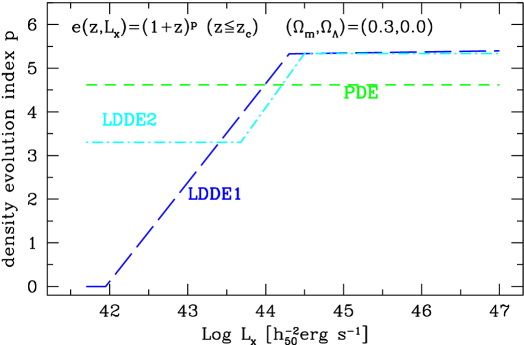
Figure 4: The behavior of the evolution indices at $z\la z_{\rm c}$ are shown as a function of luminosity for various density evolution models: PDE (short-dashed, Sect. 3.4.1), LDDE1 (long-dashed 3.4.2), and LDDE2 (dot-dashed, Sect. 4). The lines for the $(\Omega_{\rm m},\Omega_{\rm\Lambda})=$ $(0.3,0)$ case are shown.

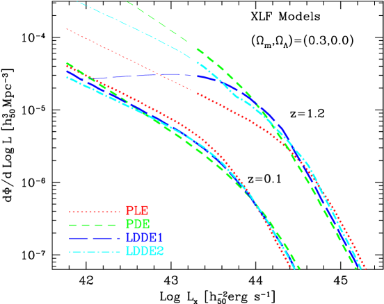
Figure 5: The behavior of the model SXLFs at z=0.1 and 1.2 are shown respectively for the PLE (dotted), PDE (short-dashed), LDDE1 (long-dashed), and LDDE2 (dot-dashed) models. For the z=1.2 curves, thick-line parts show the portion covered by the sample ($S_{\rm x14}\ga 0.2$) and the thin-line parts are extrapolations to fainter fluxes. The lines are for $(\Omega_{\rm m},\Omega_{\Lambda})=$ $(0.3,0)$.

3.5 Comparison of the data and the models

For a demonstration of the comparison between the analytical expressions and the data, we have plotted the $S^{1.5}N(>S)$ curve (the Log $N$ – Log $S$ curve plotted in such a way that the Euclidean slope becomes horizontal) for AGNs in our sample with expectations from our models (Fig. 6). Also the redshift distribution of the sample has been compared with the models in Fig. 7. These two comparisons already show intersting features. As expected, the PLE underpredicts and PDE overpredicts the number counts of lowest flux sources. In the redshift distribution, the PLE overpredicts the number of $z\la 0.08$ sources while it slightly underpredicts the $z\approx 1$ sources. Although the deviation in each redshift bin seems small, the deviations in the neighboring bins are consistent and these systematic deviations can be sensitively picked up by the KS test in the $z$ distribution (see small values of the $P_{\rm KS}$ in $z$ for the PLE model in Table 2).

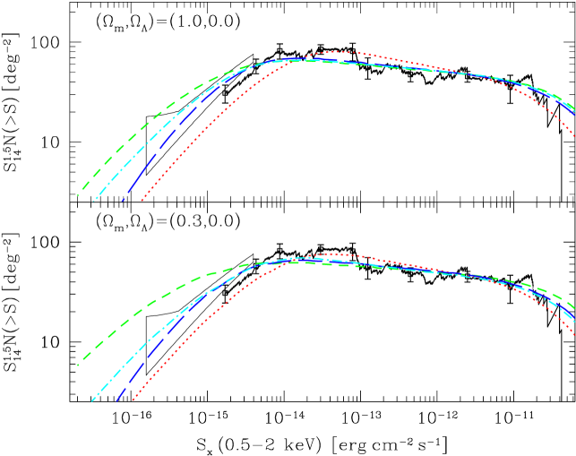
Figure 6: The $S^{1.5}N(>S)$ (a horizontal line corresponds to the Euclidean slope) curve for our sample AGNs is plotted with 90% errors at several locations and are compared with the best-fit PLE (dotted), PDE (shot-dashed), LDDE1 (long-dashed), LDDE2 (dot-dashed) models for the $(\Omega_{\rm m},\Omega_{\rm\Lambda})=$ $(1,0)$ (upper panel) and $(0.3,0)$ (lower panel). The thin-solid fish is from the fluctuation analysis of the Lockman Hole HRI data (including non-AGNs) by Hasinger et al. (has93 (1993))

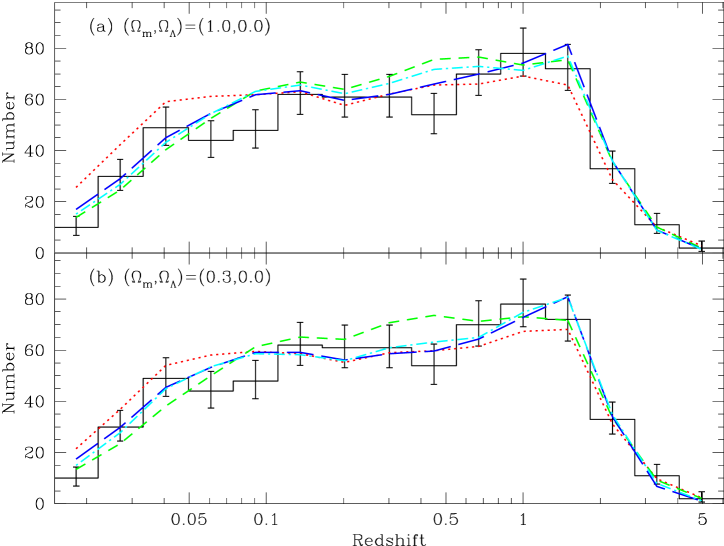
Figure 7: The redshift distribution of the AGN sample, histogrammed in equal interval in $\log\,z$, is compared with predictions from the best-fit PLE (dotted), PDE (shot-dashed), LDDE1 (long-dashed), and LDDE2 (dot-dashed) models for two sets of cosmological parameters as labeled. The assymmetric error bars correspond to approximate 1$\sigma$ Poisson errors calculated using Eqs. (7) and (11) of Gehrels (gehrels (1986)) with $S=1$.

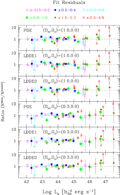
Figure 8: The full residuals of the fit are shown for the PDE, LDDE1 and LDDE2 models in two sets of cosmological parameters as labeled in each panel. The redidual in each bin has been calculated from actual number of sample AGNs falling into the bin and the model predicted number. Different symbols correspond to different redshidt bins as indicated above the top panel, which are identical to those used in Fig.3. One sigma errors have been plotted using approximations to the Poisson errors given in Gehrels (gehrels (1986)). The upper limit corresponds 2.3 objects (90% upper-limit).

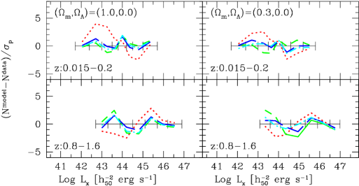
Figure 9: Residuals in the -$\chi$ space (see text) are shown for two resdhift bins, i.e., 0.015$\leq z<0.2$ and 0.8$\leq z<1.6$, where differences among different models are apparent. Different line styles correspond to different models. See caption for Fig. 5 for the line styles. The luminosity bins are shown as horizontal bars bordered by ticks.

The plots in Figs. 6 and 7 are comparisons of distributions in one-dimensional projections of a two-dimensional distribution. Only with these projected plots, one can easily overlook important residuals localized at certain locations. Thus we also would like to show the comparison in the full two-dimensional space. In literature, models are often overplotted to the binned SXLF plot calculated by the $V_{\rm a}^{-1}$ estimate like Fig. 3. However, given unavoidable biases associated with the binned $V_{\rm a}^{-1}$ estimates (see Sect. 3.2), such a plot can cause one to pick up spurious residuals. Thus we have plotted residuals in the following unbiased manner. For each model, we have calculated the expected number of objects falling into each bin ($N^{\rm model}$) and compared with the actual number of AGNs observed in the bin ($N^{\rm data}$). The full residuals in term of the ratio $N^{\rm data}/N^{\rm model}$ are plotted in Fig. 8 for the PDE, LDDE1 and LDDE2 models for two sets of cosmological parameters as labeled. The error bars correspond to 1$\sigma$ Poisson errors ($\sigma_{\rm p}$) estimated using Eqs. (7) and (11) of Gehrels (gehrels (1986)) with $S=1$. Points belonging to different redshift bins are plotted using different symbols as labeled (identical to those in Fig. 3). These residual plots show which part of the $z-L_{\rm x}$ space the given models are most representative of, which part is less constrained because of the poor statistics, and where there are systematic residuals. It seems that the models underpredict the number of AGNs in the highest luminosity bin at $2.3\leq z<4.6$ by a factor of 10, but statistical significance of the excess is still poor (2 objects against the models predictions of about 0.2). These AGNs do not constrain the fit strongly and excluding them did not change the results significantly. Also there is a scatter up to a factor of 2 from the model in $45\la{\rm Log}\,L_{\rm x}\la 46$, but no points are more than 2$\sigma$ away from either of the LDDE1 and LDDE2 models in both cosmologies.

The only data point which is more than 2$\sigma$ away from LDDE1 or LDDE2 model is the lowest luminosity bin at $1.6\leq z<2.3$ (filled triangle), i.e., $43.6\la{\rm Log}\,L_{\rm x}\la 44.2$ for ($\Omega_{\rm m},\Omega_{\Lambda}$) = (1.0,0.0) or $43.8\la{\rm Log}\,L_{\rm x}\la 44.5$ for ($\Omega_{\rm m},\Omega_{\Lambda}$) = (0.3,0.0). Both LDDE1 and LDDE2 models overpredict the number of AGNs by a factor of $\approx 2$ in both cosmologies, which are $2.2-3.8\sigma$ away. However, this location corresponds to the faintest end of the deep surveys with a certain amount of incompleteness in the identifications. Our incompleteness correction method (Sect. 2) is valid only if the unidentified source are random selections of the X-ray sources in the similar flux range. However, these sources have remained unidentified because of the difficulty of obtaining good optical spectra and not by a random cause. Thus it is possible that the incompleteness preferentially affects a certain redshift range. Actually the deficiencies were much larger in the previous version (see Fig. 8 of Hasinger et al. has99 (1999)). The discrepancies decreased after the February 1999 Keck observations of the faintest Lockman Hole sources with rather long exposures, where three of the four newly identified source turned out to be concentrated in this regime. Thus it is quite possible that the remaining four unidentified sources are also concentrated in this regime. In that case, the LDDE models can also fit to this bin within 2$\sigma$. Actually the newly identified and unidentified sources typically have very red $R-K^{\prime}$ colors (Hasinger et al. has99 (1999); Lehmann et al. 1999b ), which probably belong to a similar class to those found by Newsam et al. (newsam (1998)). If the red $R-K^{\prime}$ color comes from the stellar population of underlying galaxy, they are likely to be in a concentrated redshift regime. On the other hand, if it represents obscured AGN component, they can be in a variety of redshift range. At this moment, it is not clear whether the deficiencies in this location is due to incompleteness or indicate an actual behavior of the SXLF.

Based on the results of the 1-D and 2-D KS tests, we have rejected the PLE model. We favor the LDDE1 and LDDE2 models over the PDE model based on the KS tests and as well as the CXRB constraints (see below). It may be interesting to show the exact location where the largest discrepancies are for these models, as compared to the LDDE models. This can be most clearly shown by plotting residuals in the $-\chi=(N^{\rm model}-N^{\rm data})/\sigma_{\rm p}$ space. We have shown the $-\chi$ residuals for redshift bins where there are notable differences among these models, i.e., $0.015\leq z<0.2$ and $0.8\leq z<1.6$. These are shown in Fig. 9. For both cosmologies, the PLE model systematically shifts from overprediction to underprediction with increasing luminosity at the lowest redshift bin. At the higher resdhift bin, the opposite shift can be seen. The curve converges closer to zero at both high and low luminosity ends just because there are only small numbers of objects in these bins causing poor statistics. More apparently in the $(\Omega_{\rm m},\Omega_{\Lambda})=(0.3,0)$ universe, the PDE model also shows a significant scatter around zero.

The data in the lower luminosity part $42\la{\rm Log}\,L_{\rm x}\la 43.5$ in the lowest redshift bin ($0.015\leq z<0.2$) are crucial in rejecting the PLE model, as seen in Figs. 3 and 9. This regime, consisting of $\sim 90$ AGNs, has low SXLF values compared with the PLE extrapolation from the higher redshift data. Actually we cannot discriminate between the PLE and LDDE models for the sample of AGNs with $z<0.2$ excluded. For the $z\geq 0.2$ sample, we could find good fits (with all of the KS probabilities in $L_{\rm x}$, $z$, and 2D exceeding 0.2) in any of the PLE and LDDE models. The acceptance of the PDE model was marginal ($P_{\rm 2DKS}\sim 0.1$). The $z<0.2$ regime is mainly contributed by AGNs in the RASS-based RBS and SA-N surveys, whose flux-area space have not been explored previously. Since these samples are completely identified (see Sect. 2) and we have included all emission-line AGNs, the relatively low value in this regime is not because of the incompleteness or sampling effects. The only source of possible systematic errors which could affect the analysis would be in the flux measurements, because of the differences in details of the source detection methods among different samples. Some systematic shift of flux measurements might have occured between measurements in, e.g., the pointed and RASS data (for which there is no evidence). Thus we have made a sensitivity check by shifting the fluxes of all RBS and SA-N AGNs by $+20\%$ and $-20\%$. The flux-area relation (Fig. 1) has been modified accordingly. In either case in either value of $\Omega_{\rm m}$, the basic results did not change and especially the PLE model has been rejected with a large significance (with $P_{\rm 2DKS}$ ranging $10^{-3}-10^{-6}$).

4 Contribution to the Soft X-ray Background

In this section, we discuss the contribution of AGNs to the soft X-ray background using the various models of the SXLF. As the absolute intensity level of the extragalactic 0.5-2 keV CXRB intensity, we use the results of an ASCA-ROSAT simultaneous analysis on the ASCA LSS field (Miyaji et al. in preparation), which covers a much larger field than Miyaji et al. (cxbsp (1998)) and thus is subject to less uncertainties due to source fluctuations. There still are uncertainties in separation of the Galactic hard thermal and extragalactic components. Especially, it is still not clear whether the extragalactic component has also a soft excess at $E\la 1$ [keV] over the extrapolation from higher energies or whether the observed excess is dominated by the Galactic hard thermal component. Some authors prefer a model where the extragalactic component also contributes to the $E\la 1$ [keV] excess because fit with a single power-law plus a thermal plasma would require an unusally low metal abundance of the thermal component for a Galactic plasma (Gendreau et al. gend (1995)) and/or because many AGNs show soft excesses (e.g. Parmar et al. parmar (1999)). On the other hand, a self-consistent population synthesis model, including the AGN soft-excess below 1.3 keV, still predicts that the low-energy excess is not prominent in the 0.5-2 keV range (Miyaji et al. 1999b ), mainly because the break energy shifts to the observed photon enrgy of $E\sim 0.4$ [keV] for AGNs at $z\sim 2$, where the largest contribution to the CXRB is expected. The 0.25 keV extragalactic component measured using a shadowing of a few nearby galaxies (Warwick & Roberts shadow (1998)) is consistent with both the single power-law extrapolation case and a slight soft excess ($\Gamma\la 2$ for $E\la 1$ [keV]).

In our comparison, we use $(7.4-9.0)\times 10^{-12}$ $[{\rm erg\,s^{-1}\,cm^{-2}\,deg^{-2}}]$ as a probable range of the extragalactic 0.5-2 keV intensity, where the smaller value corresponds to the single power-law form of the extragalactic component and the larger value corresponds to the case where the extragalactic component steepens to a photon index of $\Gamma=2.3$ at $E\la 1$ [keV]. This range can be compared with the integrated intensity expected from the models.

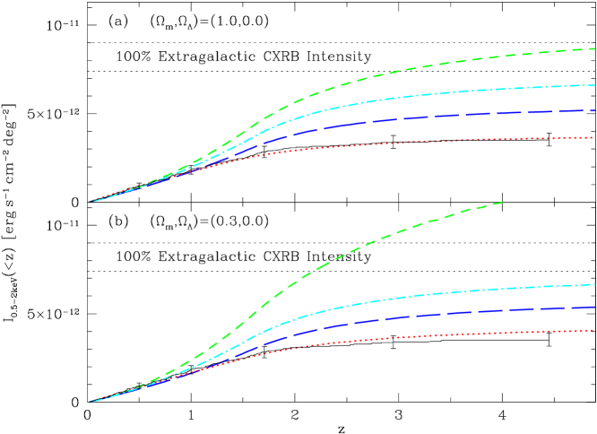
Figure 10: The cumulative 0.5-2 keV intensities $I(<z)$ are plotted as a function of redshift for the PLE, PDE, LDDE1, and LDDE2 models for two different cosmologies as labeled. See caption for Fig. 5 for line styles correponding to these four models. These curves include expected contribution from sources fainter than the survey limit using the model extrapolations. As a reference, the cumulative intensity $I(<z)$ of the AGNs in the sample (see text) is also plotted (thin solid line with 90% errors) on each panel. This curve represents the contribution of actually resolved and identified AGNs. Also the range of the 0.5-2 keV extragalactic background intensity (see text) is shown by two horizontal thin dotted lines.

In Fig. 10, we plot the cumulative soft X-ray (0.5-2 [keV]) intensities of the model AGN populations as functions of redshift, $I_{\rm 0.5-2keV}(<z)$. As a reference, we have also plotted the cumulative contribution of the resolved AGNs in the sample, estimated by $\sum_{z_{i}<z}S_{{\rm x}i}/A(S_{{\rm x}i})$, where $S_{{\rm x}i}$ is the flux of the object $i$ and $A(S_{{\rm x}i})$ is the available survey area at this flux (Fig. 1). The portion of the model curves above this line represents extrapolations to fainter fluxes than the limit of the deepest survey.

It is apparent from Fig. 10 that the PDE model produces almost 100% of the upper-estimate of the CXRB intensity, giving no room for, e.g. 10% contribution from clusters of galaxies (M99b), in the $(\Omega_{\rm m},\Omega_{\Lambda})=(1.0,0.0)$ universe. In the low density universe with $(\Omega_{\rm m},\Omega_{\Lambda})=(0.3,0.0)$, the PDE model certainly overproduces the CXRB intensity. The PLE model produces about $\sim 50\%$ of the lower estimate of the CXRB in both cosmologies. The LDDE1 model, which best describes the data in the observed regime, explains about $70\%$ of the lower estimate of the CXRB intensity. The estimates are highly dependent on how one extrapolates the SXLF to fluxes fainter than the survey limit. In view of this, we explore an alternative LDDE model, which has been adjusted to make $\approx 90\%$ of the lower estimate of the extragalactic CXRB intensity, allowing $\sim 10\%$ contribution from clusters of galaxies. This version of the LDDE model (designated as LDDE2) has a fixed minimum evolution index $p_{\rm min}$ in the LDDE formula. Then the first case of Eq. (13) is replaced by:

$$e(z,L_{\rm x})\;=\; (1+z)^{\max(p_{\rm min},{p1}-{\alpha}({\rm Log}\;{L_{\rm a}}-{\rm Log}\;L_{\rm x}))},\;$$ (14)

$$(z\leq{z_{\rm c}};L_{\rm x}<L_{\rm a}).$$

We do not intend to represent a particular physical picture behind this formula. We rather intend to search for a formally simple expression which makes 90% of the CXRB and is still consistent with our sample in the regime it covers. We have searched for models accepted by the KS tests by adjusting parameters $p_{\rm min}$, $\alpha$ and $L_{\rm a}$ by hand and fitting by the maximum-likelihood method with respect to other variable parameters, requiring that the models give an integrated intensity of $6.7\times 10^{-12}$ $[{\rm erg\,s^{-1}\,cm^{-2}\,deg^{-2}}]$. The parameter values of such LDDE2 models are listed in Table 4.

Table 4: Best-Fit LDDE2 Parameters

$(\Omega_{m},\Omega_{\Lambda})$	Parameters/KS probabilities
LDDE2	$A=(0.88\pm.06)\times 10^{-6}$; $L_{*}=0.85^{+.38}_{-.26}$
(1.0,0.0)	$\gamma_{1}=0.71\pm.14$; $\gamma_{2}=2.25\pm.10$;  $p1=4.82^{+.34}_{-.22}$
	$z_{\rm c}=1.64\pm.16$; $p2=0.$(fixed); $p_{\min}=4.0$(fixed)
	$\alpha=1.0$(fixed);  ${\rm Log}\,L_{\rm a}=44.1$ (fixed)
	$P_{\rm KS}=0.7,0.6,0.3$ (for $L$,$z$,2D)
LDDE2	$A=(1.59\pm.10)\times 10^{-6}$; $L_{*}=0.58^{+.21}_{-.14}$
(0.3,0.0)	$\gamma_{1}=0.55\pm.16$;  $\gamma_{2}=2.30\pm.08$;  $p1=5.8\pm.3$
	$z_{\rm c}=1.57\pm.12$; $p2=0.$(fixed); $p_{\min}=3.7$(fixed)
	$\alpha=2.5$ (fixed);  ${\rm Log}\,L_{\rm a}=44.6$ (fixed)
	$P_{\rm KS}=0.99,0.5,0.4$ (for $L$,$z$,2D)
LDDE2	$A=(1.48\pm.09)\times 10^{-6}$; $L_{*}=0.60^{+.23}_{-.16}$
(0.3,0.7)	$\gamma_{1}=0.57\pm.17$;  $\gamma_{2}=2.21\pm.08$; $p1=5.3\pm.3$
	$z_{\rm c}=1.59\pm.12$; $p2=0.$(fixed); $p_{\min}=3.3$(fixed)
	$\alpha=2.5$ (fixed);  ${\rm Log}\,L_{\rm a}=44.5$ (fixed)
	$P_{\rm KS}=0.7,0.8,0.4$ (for $L$,$z$,2D)

^aUnits – A: [$h_{50}^{3}\;{\rm Mpc^{-3}}$],   $L_{*}$: [$10^{44}\;h_{50}^{-2}{\rm erg\;s^{-1}}$],   Parameter errors correspond to the 90% confindence level. search (see Sect. 3.3).

By considering LDDE2, we have shown that there still is a resonable extrapolation of the AGN SXLF which makes up most of the soft CXRB. Of course this is not a unique solution. One may consider LDDE1 and LDDE2 as two possible extreme cases of how the SXLF can be extrapolated. Further implications are discussed in Sect. 6.

5 Evolution of luminous QSOs

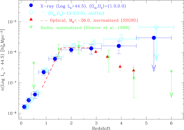
Figure 11: The comoving number density of luminous (${\rm Log}\;L_{\rm x}>44.5$) QSOs in our ROSAT AGN sample are plotted as a function of redshift for two cosmologies as labeled. The horizontal error bars indicate redshift bins and vertical error bars 1$\sigma$ errors. The top symbol of a downward arrow corresponds to the 90% (2.3 obj) upper limit. The points for $(\Omega_{\rm m},\Omega_{\Lambda})=(0.3,0.0)$ have been shifted horizontally by $+$0.1 in $z$ for display purposes. The numbers of the X-ray luminnous QSOs for the four highest redshift bins are 24[32] ($1.6\leq z<2.4$), 8[12] ($2.4\leq z<3.2$), 5[7] ($3.2\leq z<4.6$), and 0[0] ($4.6\leq z<6.0$) for $(\Omega_{\rm m},\Omega_{\Lambda})=(1.0,0.0)$ [=(0.3,0.0)]. For comparison, number density of optically-selected ($M_{\rm B}<-26$) (dashed line and filled triangles, from SSG95) and radio-selected (stars, Shaver et al. shav99 (1999)) QSOs, normalized to the soft X-ray selected QSO number density at $z\sim 2.5$ are overplotted. For the SSG95 data, this normalization corresponds to a multiplication by a factor of 7. Shaver et al. shav99 (1999) gave no absolute density.The optical and radio points are for $(\Omega_{\rm m},\Omega_{\Lambda})=(1.0,0.0)$.

In this section, we consider QSOs with high soft X-ray luminosities (${\rm Log}\;L_{\rm x}>44.5$), where the behavior of the SXLF can be traced up to high redshifts. Also in the high-luminosity regime, at least in the local universe, we observe very few absorbed AGNs, which could cause problems with the K-correction, in the local universe (e.g. Miyaji et al. 1999b ). If this tendency extends to the high redshift universe, our ROSAT sample is a good representation of luminous QSOs and the assumed single power-law of $\Gamma=2$ would be a reasonable one. Thus we here investigate the evolution of the number density of the luminous QSOs using our sample. Fig. 3 shows that the SXLF at high luminosities can be approximated by a single power-law ($\gamma\approx 2.3$) for all redshift. Assuming this power-law with a fixed slope, we have calculated the number density of AGNs above this luminosity using the fitted normalization as described above in different redshift bins. The results are plotted in Fig. 11 for two sets of cosmological parameters. Similar curves for optically and radio-selected QSOs are discussed below.

In both cases, the number density increases up to $z\sim 1.6$ and flattens beyond this redshift. In both cosmologies, the number density for $z\ga 1.7$ is consistent with no evolution. The Maximum-Likelihood fits in the $z\ga 1.7$, ${\rm Log}\;L_{\rm x}>44.5$ region gave density evolution indices ($\propto[1+z]^{p}$) of $p=0.5\pm 2.5$ and $p=0.8\pm 2.1$ for $(\Omega_{m},\Omega_{\Lambda})$ =(1.0,0.0) and (0.3,0.0) respectively. Subtle differences of the density curves seen in Fig. 11 between the two cosmologies come from two effects. Because different cosmologies give different luminosity distances, some objects which do not fall in the ${\rm Log}\;L_{\rm x}>44.5$ region for $(\Omega_{\rm m},\Omega_{\Lambda})=$ (1.0,0.0) come into the sample in lower density cosmologies. Also the comoving volume per solid angle in a certain redshift range becomes larger in lower density cosmologies, thus the number density lowers accordingly. These two effects work in the opposite sense and tend to compensate with each other, but the former effect is somewhat stronger.

It is interesting to compare this curve with similar ones from surveys in other wavelengths. In Fig. 11, we overplot number densities of optically- (Schmidt et al. ssg95 (1995), hereafter SSG95) and radio-selected (Shaver et al. shav99 (1999)) QSOs for $(\Omega_{\rm m},\Omega_{\Lambda})=$ (1.0,0.0). The densities of these QSOs have been normalized to match the ROSAT-selected QSOs at $z\sim 2.5$. This corresponds to a multiplicative factor of 7 for the SSG95 sample. Shaver et al. (shav99 (1999)) gave no absolute number density. In order to assess the statistical significance of the apparent difference of the behavior at $z>2.7$ between the ROSAT selected sample, we have used a Maximum-Likelihood fit to 17 QSOs in the sample in $z\geq 2.2$ and ${\rm Log}\,L_{\rm x}\geq 44.5$.

$$\frac{{\rm d}\;\Phi\,(L_{\rm x},z)}{{\rm d\;Log}\;L_{\rm x}}\propto L_{\rm x}^{\gamma}\cdot e(z)$$ (15)

with

$$e(z)=\left\{\begin{array}[]{ll}C&(1.7\leq z<2.7)\\ C\,\exp[-\beta(z-2.7)]&(z>2.7)\\ \end{array}\right.,$$ (16)

where $C$ is a constant. In above expression, $\beta=0$ corresponds to no evolution even for $z>2.7$ and $\beta=1$ is a good description of the rapid decrease of optically-selected QSO number density by SSG95. Fig. 11 shows that the radio-selected QSOs follow the SSG95 curve very well, but they do not have sufficient statistics to directly compare with the X-ray results. We have made a Maximum-Likelihood fit with only one free parameter: $\beta$. Fixing $\gamma$ at 2.3, we have obtained the best-fit value and 90% errors (corresponding to $\Delta{\cal L}=2.7$) of $\beta=0.1^{+.6}_{-.5}$. The result changed very little if we treat $\gamma$ as a free parameter. Setting $\beta=1$ increased the ${\cal L}$ value by 3.3 from the best-fit value. This change in ${\cal L}$ corresponds to a 93% confidence level. The probability that $\beta$ exceeds the value of 1 is $\approx 4\%$, considering only one side of the probability distribution.

We have also checked statistical significance of the difference using the density evolution-weighted $\langle V_{\rm e}^{\prime}/V_{\rm a}^{\prime}\rangle$ statistics, (Avni & Bahcall veva (1980)), which is a variant of the $\langle V^{\prime}/V_{\rm max}^{\prime}\rangle$ statistics (Schmidt vvmax (1968)) for the cases where surveys in different depths are combined. The $V_{\rm a}$ and $V_{\rm e}$ are primed to represent that they are density evolution-weighted (comoving) volumes. If we take $e(z)$ in Eq. (16) with $\beta=1$ as the weighting function, $\langle V_{\rm e}^{\prime}/V_{\rm a}^{\prime}\rangle$ will give a value of 0.5 if the sample’s redshift distribution follows the density evolution law of SSG95. An advantage of this method over the likelihood fitting is that one can check the consistency to an evolution law in a model-independent way, i.e., without assuming the shape of the luminosity function. Applying this statistics to 17 AGNs in $z\geq 2.2$, ${\rm Log}\,L_{\rm x}\geq 44.5$, we have obtained $\langle V_{\rm e}^{\prime}/V_{\rm a}^{\prime}\rangle=0.65\pm 0.07$, where the 1$\sigma$ error has been estimated by $(12N)^{-\frac{1}{2}}$ ($N$:number of objects). The same sample has given unweighted $\langle V_{\rm e}/V_{\rm a}\rangle=0.56\pm 0.07$, consistent with a constant number density. If we use a harder photon index of $\Gamma=1.7$ for the K-correction, 14 objects remain in this regime giving $\langle V_{\rm e}^{\prime}/V_{\rm a}^{\prime}\rangle=0.60\pm 0.08$. The inconsistency between the SSG95 optical results and our survey is thus marginal if high-redshift QSOs have a systematically harder spectrum.

6 Discussion

In our analysis, we have found a good description of the behavior of the SXLF from a combination of various ROSAT surveys. As explained in Sect. 3.1, our expression is for the total AGN population, including type 1 and type 2’s and for the observed 0.5-2 keV band, because of the uncertainties of contents and evolution of AGNs in various spectral classes. These have to be assumed to find the best-bet K-corrected AGN evolution in the source rest frame. A detailed discussion of this aspect is beyond the scope of this paper. An approach for the problem is to make a population synthesis modeling, e.g., composed of unabsorbed and absorbed AGNs similar to those of Madau et al. (madau94 (1994)) and Comastri et al. (coma95 (1995)) (see also Gilli gilli99 (1999) for a recent work). If one is constructing a model in a similar approach using our SXLF as a major constraint, what the model constructor should do is to calculate the expected SXLFs in the observed 0.5-2 keV band for all emission-line AGN populations (spectral classes) considered in the model (e.g. corresponding to different absorbing column densities) and then to compare the total model SXLF with our LDDE1/LDDE2 expressions. One version of our own models constructed using this approach has been shown in M99b. We do not recommend the use of the expressions in Appendix A. as the SXLF of unabsorbed AGNs for the reasons described there and Sect. 3.1.

We have found two versions of LDDE expressions consistent with our sample in the luminosity and redshift regime covered: one which produces $\sim 70\%$ of the 0.5-2 keV extragalactic CXRB (the lower etimate, see Sect. 4), and the other one which produces $\sim 90\%$, as two relatively extreme cases on extrapolation. The real behavior is probably somewhere between these two. Note that we have only calculated the contribution to the CXRB for ${\rm Log}\;L_{\rm x}>41.7$, where fits were made. Below this luminosity, we observe an excess (Fig. 3), which connects well with the SXLF of nearby Galaxies (Schmidt et al. sbv (1996); Georgantopoulos et al. geor (1999)), in the very local universe. This component has a local volume emissivity comparable or more to our sample AGNs in the 0.5-2 keV range and can contribute significantly to the soft CXRB. Because of the low luminosity, we can only detect this population in the very nearby universe in a large-area surveys like RASS. Deep small-area surveys would not give enough volume to detect them, since even the deepest part of RDS-LH can detect a ${\rm Log}\;L_{\rm x}\approx 41$ galaxy only up to $z\approx 0.1$.

The X-ray emission of this low luminosity population is probably contributed by both star-formation and by low-activity AGNs (including LINERS). Although Georgantopoulos et al. (geor (1999))’s analysis suggests that a major contribution is from Seyfert galaxies and LINERS even at these low luminosities, star-formation activity can also contribute significantly to the X-ray emission of these low-activity AGNs (see Lehmann et al. 1999a ). As one extreme scenario, we assume that the X-ray emission from these low-luminosity sources is mostly from star-formation activity and their volume emissivity is assumed to evolve like the global star-formation rate (SFR; e.g. Madau et al. madau96 (1996); Connolly et al. conn (1997)), the integrated intensity would be roughly 30-40% of the lower estimate of the CXRB intensity. Even if the evolution of these low-luminosity sources were PLE, we would not detect any of them at intermediate to high redshifts even in the deepest ROSAT Survey on the Lockman Hole. Therefore this picture is still consistent with the result that the RDS-LH did not find any starburst galaxies. If the above scenario is the case, the bahavior of the AGN component would need to be close to LDDE1 to allow room for a contribution from star-forming galaxies. In that case, the softer emission from star-formation activity could contribute to the $E\la 1$[keV] excess of the CXRB spectrum and the total extragalactic 0.5-2 [keV] intensity could be closer to the upper estimate. If on the other hand, the large apparent local volume emissivity for the low-luminosity component is produced by the local overdensity and not representative of the average present-epoch universe (e.g. Schmidt et al. sbv (1996) is from a sample within 7.5 [Mpc]) and/or the X-ray evolution is slower than the global SFR (e.g. delayed formation of LMXB, White & Ghosh white (1998)), an LDDE2-like behavior for the ${\rm Log}\;L_{\rm x}\ga 41.7$ AGN component may also be possible. A more detailed invetigation of the above scenarios and the exploration of other possibilities will be a topic of a future work.

One of the most interesting results is the evolution of luminous QSOs discussed in Sect.5. A comparison of the evolution and the global star-formation rate is discussed in Franceschini et al. (franc99 (1999)), where it is proposed that the evolution of the volume emissivity of the luminous QSOs evolves like the star-formation rate (SFR) of early-type galaxies, while that of the total AGN population (from the LDDE1 and LDDE2 models) may evolve like the SFR of all galaxies. Another interesting feature is that we find no evidence for a rapid decline of the QSO number density at high redshift. The SSG95-like decrease at $z>2.7$ is marginally rejected. The difference may be caused by different selection criteria. SSG95 have selected QSOs by the Ly$\alpha$ luminosity and their QSOs are representative of more luminous QSOs ($M_{\rm B}<-26$). Recently Wolf et al. (wolf (1999)) reported a similar tendency in their sample of QSOs from one of their CADIS fields, which typically have lower luminosities than the SSG95 sample. Our X-ray selected AGNs with ${\rm Log}\;L_{\rm x}>44.5$ have a seven times higher space density than SSG95 at $z\sim 2.5$ and thus are sampling lower luminosity QSOs than SSG95. Thus if the behavior of our ROSAT-selected QSOs and those of Wolf et al. (wolf (1999)) is really flat, this can be indicative of different formation epochs for lower and higher mass black holes. Adding more deep ROSAT surveys would enable us to trace the evolution in this regime with a better statistical significance. The upcoming Chandra and XMM Surveys would extend the analysis to lower-luminsoity objects at the highest redshifts as well as enabling us to give spectral information to separate the K-effect and the actual evolution of the number density.

7 Conclusion

We summarize the main conclusions of our analysis of the $\sim 690$ AGNs from the ROSAT surveys in a wide range of depths:

1. Like previous works, we find a strong evolution of the SXLF up to $z\sim 1.5$ and a levelling-off beyond this redshift.

2. We have tried to find a simple analytical description of the overall SXLF. Our combined sample rejects the classical PLE model with high significance. The PDE model has been marginally rejected statistically and also overproduces the soft CXRB.

3. We have found that an LDDE form (LDDE1), where the evolution rate is lower at low luminosities, gives an excellent fit to the overall SXLF. The extrapolation of the LDDE1 form produces $\approx 60-70\%$ of the estimated extragalactic soft CXRB.

4. Another form of LDDE (LDDE2), which equally well describes the overall SXLF from our sample, produces $\approx 90\%$ of the extragalactic soft CXRB. These two LDDE models may be considered as two possible extreme cases when one considers the origin of the soft CXRB.

5. The evolution of the number density of luminous QSOs in our sample has been compared with that of optically- and radio-selected QSOs. Our data are consistent with constant number density at $z>2.7$, while optically- and radio-selected QSOs show a rapid decline. The statistical significance of this difference is just above 2$\sigma$. Including more deep ROSAT surveys would trace the behavior with a better significance.

Appendix A SXLF of the ’type 1’ AGN sample

In the main part of this paper, we have concentrated on the SXLF expression for the mixture of type 1 and type 2 AGNs for the reasons explained in Sect.3.1. However, since previous works in literature mainly give expression for only type 1 AGNs (with broad permitted lines), it is of significant historical interest to investigate the SXLF properties for only type 1 AGNs. Because our samples come from several different sources and every subsample has its own criteria for classifying AGNs into subclasses, our expressions given here should not be used for any quantitative work (e.g. using it as a starting point of a population synthesis modeling under an assumption that they represent the unabsorbed AGNs) without assessment of possible biases described in Sect.3.1.

We have defined the ’type 1’ AGN sample as follows. We have included AGNs explicitly classified in the original catalogs as Seyfert 1-1.5’s, BLRGs, and QSOs, while excluded those classified as Seyfert 1.8-2, NELGs, and Narrow-line Seyfert 1’s (NLS1). The NLS1’s have been excluded since they would not have been included in the ’broad-line’ AGN samples in the previous works, especially those with low-quality optical spectra. A number of RBS objects classifed simply as ’AGNs’ have been ckecked with the NED database and/or the original spectra for the subclassifications. For the Lockman Hole sample, we have included objects with ID classes (a)-(c) (see Schmidt et al. rds2 (1998)) and excluded (d)-(e). For the Marano sample, those classified as AGNs in Zamorani et al marano (1999) have been assumed to be type 1 AGNs unless otherwise stated, since type 2 AGNs have been explicitly noted. The AGNs which have not been subclassified using the above procedure have been excluded from our ’type 1’ sample. The fraction of AGNs included in this ’type 1’ sample are 98% (RBS), 90% (SA-N), 93%(RIXOS), 88% (NEP+Marano+UKD), and 85% (LH) respectively.

Table 5: Best-fit Parameters for the ’type 1’ Sample

Model	Parameters/KS probabilities
$(\Omega_{m},\Omega_{\Lambda})$
PLE	$A=(4.8\pm.3)\times 10^{-6}$; $L_{*}=0.28\pm.09$
(1.0,0.0)	$\gamma_{1}=0.43\pm.19$; $\gamma_{2}=2.30\pm.11$; $p1=3.0\pm.2$
	$z_{\rm c}=1.45\pm.19$; $p2=0.3^{+.6}_{-.8}$
	$P_{\rm KS}=5\;10^{-4},3\;10^{-4},7\;10^{-5}$ (for $L$,$z$,2D)
PLE	$A=(3.6\pm.2)\times 10^{-6}$; $L_{*}=0.34\pm.10$
(0.3,0.0)	$\gamma_{1}=0.41\pm.19$; $\gamma_{2}=2.31\pm.11$; $p1=3.0\pm.2$
	$z_{\rm c}=1.47\pm.28$; $p2=0.46\pm.7$
	$P_{\rm KS}=.02,.008,.002$ (for $L$,$z$,2D)
LDDE1	$A=(1.40\pm.10)\times 10^{-6}$; $L_{*}=0.60^{+.32}_{-.19}$
(1.0,0.0)	$\gamma_{1}=0.62\pm.20$; $\gamma_{2}=2.25\pm.09$; $p1=5.4\pm.3$
	$z_{\rm c}=1.55\pm.15$; $p2=0.0$ (fixed)
	$\alpha=2.5\pm.8$;  ${\rm Log}L_{\rm a}=44.2$ (fixed)
	$P_{\rm KS}=0.6,0.6,0.6$ (for $L$,$z$,2D);
LDDE1	$A=(1.52\pm.10)\times 10^{-6}$; $L_{*}=0.55^{+.35}_{-.20}$
(0.3,0.0)	$\gamma_{1}=0.62\pm.23$; $\gamma_{2}=2.17\pm.08$; $p1=5.3\pm.3$
	$z_{\rm c}=1.62\pm.14$;  $p2=0.0$ (fixed)
	$\alpha=3.0\pm.9$;  ${\rm Log}L_{\rm a}=44.2$ (fixed)
	$P_{\rm KS}=0.3,0.8,0.3$ (for $L$,$z$,2D)

See Captions for Tables 2 and 3 for units of the parameters and other notes.

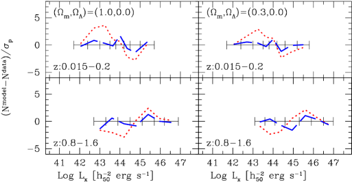
Figure 12: Same as Fig. 9 except that this is for the ’type 1’ AGN sample and that only PLE and LDDE1 models are plotted.

We have only considered the PLE and LDDE1 models in this appendix. Table 5 shows best-fit parameters and KS probabilities (see main text for details). Table 5 shows that PLE is still rejected with a large significance for both cosmologies, while finding good fits with the LDDE1 form. A plot similar to Fig.9 is shown for the ’type 1’ AGN sample in Fig.12.