Large-scale structure in the Lyman-$\alpha$ forest II: analysis of a group of ten QSOs

Abstract

The spatial distribution of Ly$\alpha$ forest absorption systems towards ten QSOs has been analysed to search for large-scale structure over the redshift range $2.2<z<3.4$. The QSOs form a closely spaced group on the sky and are concentrated within a $1$ deg² field. We have employed a technique based on the first and second moments of the transmission probability density function which is capable of identifying and assessing the significance of regions of over- or underdense Ly$\alpha$ absorption. We find evidence for large-scale structure in the distribution of Ly$\alpha$ forest absorption at the $>99$ per cent confidence level. In individual spectra we find overdense Ly$\alpha$ absorption on scales of up to $1200$ km s^-1. There is also strong evidence for correlated absorption across line of sight pairs separated by $<3$ h^-1 proper Mpc ($q_{0}=0.5$). For larger separations the cross-correlation signal becomes progressively less significant.

1 Introduction

The Ly$\alpha$ forest seen in the spectra of distant QSOs may constitute a substantial fraction of the baryonic content of the Universe [Rauch & Haehnelt (1995)] and its evolution can be traced over most of the history of the Universe. Every QSO absorption spectrum provides us with a representative, albeit one-dimensional sample of the baryonic matter distribution, unaffected by any luminosity bias. The intimate relationship of the absorbing gas with the thermal, chemical, and dynamical history of the Universe makes the Ly$\alpha$ forest a versatile, but not always user-friendly tool in the study of cosmology.

The observational and theoretical advances of the past decade have significantly altered our understanding of the Ly$\alpha$ forest. The advent of HST’s UV spectroscopic capabilities led to the first detailed analyses of the low redshift Ly$\alpha$ forest ([Morris et al. (1991)]; [Bahcall et al. (1991)]). Subsequently, using multislit spectroscopy and deep imaging of galaxies in the fields of QSOs, significant numbers of coincidences between the redshifts of absorption lines and galaxies were found at $z\mathrel{\mathchoice{\vbox{\offinterlineskip\halign{\hfil$\reset@font\displaystyle#$\hfil\cr<\cr\sim\cr}}}{\vbox{\offinterlineskip\halign{\hfil$\reset@font\textstyle#$\hfil\cr<\cr\sim\cr}}}{\vbox{\offinterlineskip\halign{\hfil$\reset@font\scriptstyle#$\hfil\cr<\cr\sim\cr}}}{\vbox{\offinterlineskip\halign{\hfil$\reset@font\scriptscriptstyle#$\hfil\cr<\cr\sim\cr}}}}1$. Several groups determined that galaxies have absorption cross-sections of $\sim 200$ h^-1 kpc ([Lanzetta et al. (1995)]; [Le Brun et al. (1996)]; [Bowen et al. (1996)]). Moreover, ?), ?), and ?) found an anti-correlation of the Ly$\alpha$ rest equivalent width, $W$, with the distance of the absorbing galaxy to the line of sight of the QSO as well as a slight correlation with luminosity [Chen et al. (1998)]. Thus ?) confirmed earlier results that the extended gaseous halos of galaxies are directly responsible for a significant fraction of the Ly$\alpha$ forest at $z\mathrel{\mathchoice{\vbox{\offinterlineskip\halign{\hfil$\reset@font\displaystyle#$\hfil\cr<\cr\sim\cr}}}{\vbox{\offinterlineskip\halign{\hfil$\reset@font\textstyle#$\hfil\cr<\cr\sim\cr}}}{\vbox{\offinterlineskip\halign{\hfil$\reset@font\scriptstyle#$\hfil\cr<\cr\sim\cr}}}{\vbox{\offinterlineskip\halign{\hfil$\reset@font\scriptscriptstyle#$\hfil\cr<\cr\sim\cr}}}}1$. However, there is evidence that this may only be true for stronger lines ($W\mathrel{\mathchoice{\vbox{\offinterlineskip\halign{\hfil$\reset@font\displaystyle#$\hfil\cr>\cr\sim\cr}}}{\vbox{\offinterlineskip\halign{\hfil$\reset@font\textstyle#$\hfil\cr>\cr\sim\cr}}}{\vbox{\offinterlineskip\halign{\hfil$\reset@font\scriptstyle#$\hfil\cr>\cr\sim\cr}}}{\vbox{\offinterlineskip\halign{\hfil$\reset@font\scriptscriptstyle#$\hfil\cr>\cr\sim\cr}}}}0.3$ Å) and that the weaker absorption lines trace the large-scale gaseous structures in which galaxies are presumably embedded ([Le Brun & Bergeron (1998)]; [Tripp et al. (1998)]).

At high redshift, the discovery of measurable amounts of C IV associated with 75 per cent of all Ly$\alpha$ absorbers with coloumn density $N($H I$)>10^{14.5}$ cm^-2 ([Cowie et al. (1995)]; [Songaila & Cowie (1996)]) in high-quality spectra obtained with the HIRES spectrograph on the Keck 10-m telescope has challenged the original notion of the Ly$\alpha$ forest arising in pristine, primordial gas. However, ?) found almost no associated C IV absorption for systems with $N($H I$)<10^{14}$ cm^-2 and derived $[{\rm C}/{\rm H}]<-3.5$, about a factor of ten smaller than inferred by ?) (see also [Davé et al. (1998a)]), suggesting a sharp drop in the metallicity of the Ly$\alpha$ forest at $N($H I$)\approx 10^{14}$ cm^-2. Nevertheless, the metallicity of the higher column density systems raises the possibility of an association of these systems with galaxies at high redshift. Using the same C IV lines to resolve the structure of the corresponding blended Ly$\alpha$ lines, ?) have shown that the clustering properties of these systems are consistent with the clustering of present-day galaxies if the correlation length of galaxies is allowed to evolve rapidly with redshift ($\epsilon\approx 2.4$).

On the theoretical side, models have progressed from the early pressure-confined ([Sargent et al. (1980)]; [Ostriker & Ikeuchi (1983)]; [Ikeuchi & Ostriker (1986)]; [Williger & Babul (1992)]) and dark matter mini-halo ([Rees (1986)]; [Ikeuchi (1986)]) scenarios to placing the Ly$\alpha$ forest fully within the context of the theory of CDM dominated, hierarchical structure formation. Both semi-analytical ([Petitjean et al. (1995)]; [Bi & Davidsen (1997)]; [Hui et al. (1997)]; [Gnedin & Hui (1998)]) and full hydrodynamical numerical simulations ([Cen et al. (1994)]; [Zhang et al. (1995)]; [Miralda-Escudé et al. (1996)]; [Hernquist et al. (1996)]; [Wadsley & Bond (1997)]; [Theuns et al. (1998)]) of cosmological structure formation, which include the effects of gravity, photoionisation, gas dynamics, and radiative cooling, have shown the Ly$\alpha$ forest to arise as a natural by-product in the fluctuating but continuous medium which forms by gravitational growth from initial density perturbations. The simulations are able to match many of the observed properties of the Ly$\alpha$ absorption to within reasonable accuracy ([Miralda-Escudé et al. (1996)]; [Zhang et al. (1997)]; [Davé et al. (1997)]; [Davé et al. (1998b)]; [Mücket et al. (1996)]; [Riediger et al. (1998)]; [Theuns et al. (1998)]). A common feature of all the simulations is that the absorbing structures exhibit a variety of geometries, ranging from low density, sheet-like and filamentary structures to the more dense and more spherical regions where the filaments interconnect and where, presumably, galaxies form. The dividing line between these different geometries lies in the range $10^{14}$ cm${}^{-2}\mathrel{\mathchoice{\vbox{\offinterlineskip\halign{\hfil$\reset@font\displaystyle#$\hfil\cr<\cr\sim\cr}}}{\vbox{\offinterlineskip\halign{\hfil$\reset@font\textstyle#$\hfil\cr<\cr\sim\cr}}}{\vbox{\offinterlineskip\halign{\hfil$\reset@font\scriptstyle#$\hfil\cr<\cr\sim\cr}}}{\vbox{\offinterlineskip\halign{\hfil$\reset@font\scriptscriptstyle#$\hfil\cr<\cr\sim\cr}}}}N\mathrel{\mathchoice{\vbox{\offinterlineskip\halign{\hfil$\reset@font\displaystyle#$\hfil\cr<\cr\sim\cr}}}{\vbox{\offinterlineskip\halign{\hfil$\reset@font\textstyle#$\hfil\cr<\cr\sim\cr}}}{\vbox{\offinterlineskip\halign{\hfil$\reset@font\scriptstyle#$\hfil\cr<\cr\sim\cr}}}{\vbox{\offinterlineskip\halign{\hfil$\reset@font\scriptscriptstyle#$\hfil\cr<\cr\sim\cr}}}}10^{15}$ cm^-2 ([Cen & Simcoe (1997)]; [Zhang et al. (1998)]).

Thus a consistent picture may be emerging: absorption lines with $N\mathrel{\mathchoice{\vbox{\offinterlineskip\halign{\hfil$\reset@font\displaystyle#$\hfil\cr>\cr\sim\cr}}}{\vbox{\offinterlineskip\halign{\hfil$\reset@font\textstyle#$\hfil\cr>\cr\sim\cr}}}{\vbox{\offinterlineskip\halign{\hfil$\reset@font\scriptstyle#$\hfil\cr>\cr\sim\cr}}}{\vbox{\offinterlineskip\halign{\hfil$\reset@font\scriptscriptstyle#$\hfil\cr>\cr\sim\cr}}}}10^{14.5}$ cm^-2 are closely associated with the large, spherical outer regions of galaxies, cluster strongly on small velocity scales along the line of sight [Fernández-Soto et al. (1996)], and have been contaminated with metals by supernovae from a postulated Population III (e.g. [Miralda-Escudé & Rees (1997)]) or by galaxy mergers (e.g. [Gnedin (1998)]); whereas lower column density lines trace the interconnecting, filamentary structures of the intergalactic medium.

Whatever the case may be, it seems likely that the large-scale distribution of the Ly$\alpha$ absorption holds important clues to its origin. Ly$\alpha$ absorbers are probably fair tracers of the large-scale cosmic density field and should thus be able to constrain structure formation models. To investigate further the connection of the Ly$\alpha$ forest with cosmological structure we study in this paper its large-scale structure both in velocity and real space by considering a close group of ten QSOs. The QSOs are contained within a $\sim 1$ deg² field so that the Ly$\alpha$ forest is probed on Mpc scales.

There have been many studies of the clustering properties of the Ly$\alpha$ forest. ?) was the first to report a weak signal in the two-point correlation function of fitted absorption lines on scales of $\mathrel{\mathchoice{\vbox{\offinterlineskip\halign{\hfil$\reset@font\displaystyle#$\hfil\cr<\cr\sim\cr}}}{\vbox{\offinterlineskip\halign{\hfil$\reset@font\textstyle#$\hfil\cr<\cr\sim\cr}}}{\vbox{\offinterlineskip\halign{\hfil$\reset@font\scriptstyle#$\hfil\cr<\cr\sim\cr}}}{\vbox{\offinterlineskip\halign{\hfil$\reset@font\scriptscriptstyle#$\hfil\cr<\cr\sim\cr}}}}100$ km s^-1. This result was later confirmed ([Ostriker et al. (1988)]; [Chernomordik (1995)]; [Cristiani et al. (1995)]; [Kulkarni et al. (1996)]; [Cristiani et al. (1997)]; [Khare et al. (1997)]), and some investigators found considerably stronger signals ([Ulmer (1996)]; [Fernández-Soto et al. (1996)]). There have also been detections on larger scales. ?) used a nearest neighbour statistic to derive correlations on scales of $0.5$–$3$ h^-1 Mpc. ?) employed the discrete wavelet transform to demonstrate the existence of clusters on scales of $10$–$20$ h^-1 Mpc in the Ly$\alpha$ forest at a significance level of $2$–$4\sigma$ and that the number density of these clusters decreases with increasing redshift. More recently, they observed non-Gaussian behaviour of Ly$\alpha$ forest lines on scales of $5$–$10$ h^-1 Mpc at a confidence level larger than 95 per cent [Pando & Fang (1998)]. ?) even reported $60$ and $130$ h^-1 Mpc as characteristic scales of the Ly$\alpha$ forest. All of these studies however are based on analyses of individual lines of sight.

By comparing the absorption characteristics in two (or more) distinct, but spatially close lines of sight, it is possible to investigate directly the real space properties of Ly$\alpha$ systems on various scales. The multiple images of gravitationally lensed QSOs have been used to establish firm lower limits on the sizes of Ly$\alpha$ clouds. ?) found that the Ly$\alpha$ forests of the two images of HE 1104–1805 (separation $3.0$ arcsec) are virtually identical and inferred a $2\sigma$ lower limit of $50$ h^-1 kpc on the diameter of Ly$\alpha$ clouds, assumed to be spherical, at $z=2.3$. More information on the sizes of Ly$\alpha$ absorbers has been gained from the studies of close QSO pairs with separations of several arcsec to $\sim 7$ arcmin. All of the most recent analyses have concluded that Ly$\alpha$ absorbers have diameters of a few hundred kpc ([Fang et al. (1996)]; [Dinshaw et al. (1997)]; [Dinshaw et al. (1998)]; [Petitjean et al. (1998)]; [D’Odorico et al. (1998)]) and ?) found that correlations among neighbouring lines of sight persist for separations up to $0.5$–$0.8$ h^-1 Mpc for lines with $W>0.4$ Å. A tentative detection of increasing cloud size with decreasing redshift (as would be expected for absorbers expanding with the Hubble flow) was reported by ?) and ?). The possibility remains however, that the coincidences of absorption lines are due to spatial clustering of absorbers and that the inferred ‘sizes’ in fact are an indication of their correlation length ([Dinshaw et al. (1998)]; [Cen & Simcoe (1997)]) as may be evidenced by the correlation of the estimated ‘size’ with line of sight separation found by ?).

Analyses to determine the shape of absorbers, as proposed e.g. by ?), have so far been inconclusive. Several authors agree that the current data are incompatible with uniform-sized spherical clouds but are unable to decisively distinguish between spherical clouds with a distribution of sizes, flattened disks, or filaments and sheets ([Fang et al. (1996)]; [Dinshaw et al. (1997)]; [D’Odorico et al. (1998)]). However, from the analysis of a QSO triplet ?) found evidence that lines with $W>0.4$ Å arise in sheets.

For still larger line of sight separations most work has concentrated on metal absorption. ?), e.g., used a group of 25 QSOs contained within a $\sim 1$ deg² region to identify structure in C IV absorption on the scale of $15$–$35$ h^-1 Mpc. Within this group, a subset of ten QSOs is suitable for studying the large-scale structure of the Ly$\alpha$ forest. A cross-correlation analysis of these data, performed by ?), revealed a $3.7\sigma$ excess of line-pairs at velocity splittings $50<\Delta v<100$ km s^-1. Thus [Williger et al. (1999)] concluded that the Ly$\alpha$ forest seems to exhibit structure on the scale of $\sim 10$ h^-1 Mpc in the plane of the sky. However there was no excess at smaller velocity splittings and no dependence of the signal on angular separation was found.

Finally, the largest line of sight separations were investigated by ?), who studied a group of four QSOs, projected within $2\hbox{$.\!\!^{\circ}$}8$ on the sky. Probing scales of $\sim 30$ h^-1 Mpc in the plane of the sky, no significant cross-correlation signal was found out to a velocity separation of $10^{4}$ km s^-1.

From the results outlined above it appears that the Ly$\alpha$ forest shows significant correlations across lines of sight at all but the largest scales probed. In this paper we identify more precisely the upper limit of these correlations. To this end we re-analyse the group of ten QSOs of [Williger et al. (1999)] in the South Galactic Pole region. We employ a novel technique which is based on the statistics of the transmitted flux rather than the statistics of fitted absorption lines [Liske et al. (1998)] (hereafter paper I). The South Galactic Cap region has one of the highest known QSO densities in the sky and the dataset is the most useful for large-scale structure studies of the Ly$\alpha$ forest published so far. We find evidence for a transition from strong correlations for proper line of sight separations $<3$ h^-1 Mpc to a vanishing correlation for line of sight separations $>6$ h^-1 Mpc.

The rest of the paper is organised as follows: in Section 2 we briefly describe the data. Section 3 outlines the method of analysis and its main advantages over a ‘traditional’ two-point correlation function analysis. Our results are presented in Section 4 and discussed in Section 5.

2 The Data

The data were gathered as part of a larger survey designed to reveal the large-scale clustering properties of C IV systems [Williger et al. (1996)]. The observations were made on the CTIO 4-m telescope using the Argus multifibre spectrograph. The instrumental resolution was $\sim 2$ Å and the signal-to-noise ratio per pixel reached up to 40 per 1 Å pixel. For a complete description of the observations and the reduction process we refer the reader to ?).

Of the original sample of $25$ QSO spectra only $14$ cover any part of the region between the Ly$\alpha$ and Ly$\beta$ emission lines. In order to avoid the proximity effect we exclude from the analysis those parts of the spectra which lie within 3000 km s^-1 of the Ly$\alpha$ emission line. This leaves us with $11$ spectra. We have excluded an additional spectrum from the analysis (Q0043–2606) because of its low S/N and small wavelength coverage. We are thus left with the same sample as used by ?). We list these QSOs, their positions and redshifts in Table 2 and show their distribution in the sky in Fig. 2. The data cover $2.17<z<3.40$.

Table 2: QSOs analysed.

Object	$\alpha_{1950}$	$\delta_{1950}$	$z_{em}$
	$\!\!\!h\ m\quad\ s$	∘   ′   ′′
Q0041–2638	$00\;41\;15.19$	$-26\;38\;35.9$	$3.053$
Q0041–2707	$00\;41\;24.38$	$-27\;07\;54.3$	$2.786$
Q0041–2607	$00\;41\;31.11$	$-26\;07\;41.7$	$2.505$
Q0041–2658	$00\;41\;38.38$	$-26\;58\;30.0$	$2.457$
Q0042–2627	$00\;42\;06.42$	$-26\;27\;45.3$	$3.289$
Q0042–2639	$00\;42\;08.20$	$-26\;39\;25.0$	$2.98$
Q0042–2656	$00\;42\;24.89$	$-26\;56\;34.4$	$3.33$
Q0042–2714	$00\;42\;44.12$	$-27\;14\;56.6$	$2.36$
Q0042–2657	$00\;42\;52.29$	$-26\;57\;15.3$	$2.898$
Q0043–2633	$00\;43\;03.10$	$-26\;33\;33.6$	$3.44$

The angular separations range from $6.1$ to $69.2$ arcmin or $1.4$ to $16.3$ h^-1 proper Mpc and the emission redshifts range from $2.36$ to $3.44$.

Figure 2: Distribution of QSOs in the sky. The field is centered on $\alpha=00^{{\rm h}}42^{{\rm m}}10^{{\rm s}}$ and $\delta=-26\hbox{${}^{\circ}$}40\hbox{${}^{\prime}$}$ (B1950). Stars mark the positions of the QSOs listed in Table 2 and emission redshifts are indicated.

3 Analysis

The method of analysis used in this work is described in detail in paper I. Our technique does not rely on the statistics of individual absorption lines but rather identifies local over- or underdensities of Ly$\alpha$ absorption using the statistics of the transmitted flux. In order to identify large-scale features in a normalised spectrum of the Ly$\alpha$ forest we convolve the spectrum with a smoothing function. In fact, we smooth the spectrum on all possible scales. On the smallest possible scale ($=1$ pixel) the spectrum remains essentially unchanged whereas on the largest possible scale ($=$ number of pixels in the spectrum) the whole spectrum is compressed into a single number akin to $1-D_{A}$, where $D_{A}$ is the flux deficit parameter [Oke & Korycansky (1982)]. When plotted in the wavelength–smoothing scale plane, this procedure results in the ‘transmission triangle’ of the spectrum. The base of the triangle is the original spectrum itself and the tip is the single value which results from smoothing the spectrum on the largest possible scale. Thus a cluster of absorption lines will be enhanced by filtering out the ‘high-frequency noise’ of the individual absorption lines. We use a Gaussian as the smoothing function and denote the smoothed spectrum by $G(\lambda,\sigma_{\rm s})$.

We are interested in identifying local fluctuations around the mean Ly$\alpha$ transmission and in assessing their statistical significance. To this end we have calculated both the expected mean, $\langle G\rangle$, and variance, $\sigma_{G}^{2}$, of the Ly$\alpha$ transmission as functions of wavelength and smoothing scale in paper I. The calculations are based on the simple null-hypothesis that any Ly$\alpha$ forest spectrum can be described by a collection of individual absorption lines whose parameters are uncorrelated. Thus, in particular, the null-hypothesis presumes an unclustered Ly$\alpha$ forest. The derivation also uses the observationally determined functional form of the distribution of the absorption line parameters, for redshift $z$, column density $N$, and Doppler parameter $b$,

$$\eta(z,N,b)\propto(1+z)^{\gamma}N^{-\beta}\exp\left[\frac{-(b-\mu_{b})^{2}}{2\sigma_{b}^{2}}\right]$$ (1)

for $b>b_{\rm cut}$ ([Carswell et al. (1984)]; [Lu et al. (1996)]; [Kim et al. (1997)]; [Kirkman & Tytler (1997)]) and the results are given in terms of its parameters:

$$\langle G\rangle(\lambda,\sigma_{\rm s})={\rm e}^{-B(\frac{\lambda}{\lambda_{\alpha}})^{\gamma+1}},$$ (2)

and

$$\sigma_{G}^{2}(\lambda,\sigma_{\rm s})=\frac{\sigma_{n}^{2}(\lambda)}{2\sqrt{\pi}\;\sigma_{\rm s}/ps}+\frac{\sigma_{{\rm e}^{-\tau}}^{2}(\lambda)}{\sqrt{2\frac{\sigma_{\rm s}^{2}+\sigma_{\rm LSF}^{2}}{q^{2}(\lambda)}+1}},$$ (3)

where

$$\sigma_{{\rm e}^{-\tau}}^{2}={\rm e}^{-2^{\beta-1}B(\frac{\lambda}{\lambda_{\alpha}})^{\gamma+1}}-{\rm e}^{-2B(\frac{\lambda}{\lambda_{\alpha}})^{\gamma+1}}.$$ (4)

$\sigma_{n}$ denotes the noise of a spectrum, $\sigma_{\rm LSF}$ the width of the line spread function, $ps$ the pixel size in Å, and $\lambda_{\alpha}=1215.67$ Å. $q$ is the intrinsic width of the auto-covariance function of a spectrum (approximated as a Gaussian, see also paper I). In paper I we tested the analytic expressions above against extensive numerical simulations and found excellent agreement. Given that the Gunn-Peterson optical depth is limited to $\tau_{\rm GP}\mathrel{\mathchoice{\vbox{\offinterlineskip\halign{\hfil$\reset@font\displaystyle#$\hfil\cr<\cr\sim\cr}}}{\vbox{\offinterlineskip\halign{\hfil$\reset@font\textstyle#$\hfil\cr<\cr\sim\cr}}}{\vbox{\offinterlineskip\halign{\hfil$\reset@font\scriptstyle#$\hfil\cr<\cr\sim\cr}}}{\vbox{\offinterlineskip\halign{\hfil$\reset@font\scriptscriptstyle#$\hfil\cr<\cr\sim\cr}}}}0.04$ [Webb et al. (1992)] and given the number density of metal lines, we can safely neglect the effects of both of these potential contributors to $\tau_{\rm eff}$ in equation (2).

A potential source of error in the method used here is its sensitivity to the adopted continuum fit. A small error in the zeroth or first order of the fit introduces an arbitrary offset from the expected mean transmission. However, this is easily dealt with by determining the normalisation of the mean optical depth, $B$, for each spectrum individually:

$$B=-\left(\frac{\lambda_{\alpha}}{\lambda_{\rm c}}\right)^{\gamma+1}\ln[G(\lambda_{\rm c},\sigma_{\rm s,max})],$$ (5)

where $\sigma_{\rm s,max}$ denotes the largest possible smoothing scale and $\lambda_{\rm c}$ is the central wavelength of the spectrum. Thus we fix the normalisation for each spectrum at the tip of its transmission triangle.

Before we can evaluate expressions (2) and (3) we need the values of several other parameters: $\gamma$ was determined by ?) for the present data to be $2.5$ and we take $\beta$ from recent high resolution studies as $1.5$ ([Hu et al. (1995)]; [Lu et al. (1996)]; [Kim et al. (1997)]; [Kirkman & Tytler (1997)]). As in paper I we determined the width of the auto-covariance function of a ‘perfect’ spectrum (i.e. before it passes through the instrument), $q$, from simulations. We simulated each spectrum of the dataset $100$ times in accordance with the null-hypothesis (see also paper I), using the $\gamma$ and $\beta$ values as above and $\mu_{b}=30$ km s^-1, $\sigma_{b}=8$ km s^-1 and $b_{\rm cut}=18$ km s^-1 ([Hu et al. (1995)]; [Lu et al. (1996)]; [Kim et al. (1997)]; [Kirkman & Tytler (1997)]). The simulated data have the same resolution as the real data but a constant (conservative) S/N of $20$. The simulations are normalised to give the same mean effective optical depth as the real data.

With the values of all the parameters in place, we can transform a given transmission triangle into a ‘reduced’ transmission triangle by

$$RG(\lambda,\sigma_{\rm s})=\frac{G-\langle G\rangle}{\sigma_{G}}.$$ (6)

The reduced transmission triangle shows the residual fluctuations of the Ly$\alpha$ transmission around its mean in terms of their statistical significance.

There are several advantages of the method outlined above over a more ‘traditional’ approach involving absorption line fitting and construction of the two-point correlation function. Most importantly, our technique does not require arduous line-fitting and side-steps all difficulties arising from line-blending [Fernández-Soto et al. (1996)]. In paper I we demonstrated that for simulated data our technique is significantly more sensitive to the presence of large-scale structure than a two-point correlation function analysis, especially at intermediate resolution. Moreover, numerical simulations of cosmological structure formation ([Cen et al. (1994)]; [Miralda-Escudé et al. (1996)]; [Hernquist et al. (1996)]; [Zhang et al. (1995)]; [Wadsley & Bond (1997)]; [Theuns et al. (1998)]) indicate that at least the low column density forest arises in a fluctuating but continuous medium so that a given absorption line may not correspond to a well-defined individual ‘cloud’. Thus a method of analysis based on the statistics of the transmitted flux itself is most appropriate and intuitive.

A high signal-to-noise ratio in the QSO spectra is not of great importance for the analysis itself (as the noise is quickly smoothed over, see equation 3), but it is important for reliable continuum fitting. Uncertainties in the placement of the continuum have already been dealt with above (equation 5). The second source of uncertainty are the values of the parameters of equation (1) and we will discuss the pertaining effects in Sections 4.2 and 4.3.

4 Results

4.1 Single lines of sight

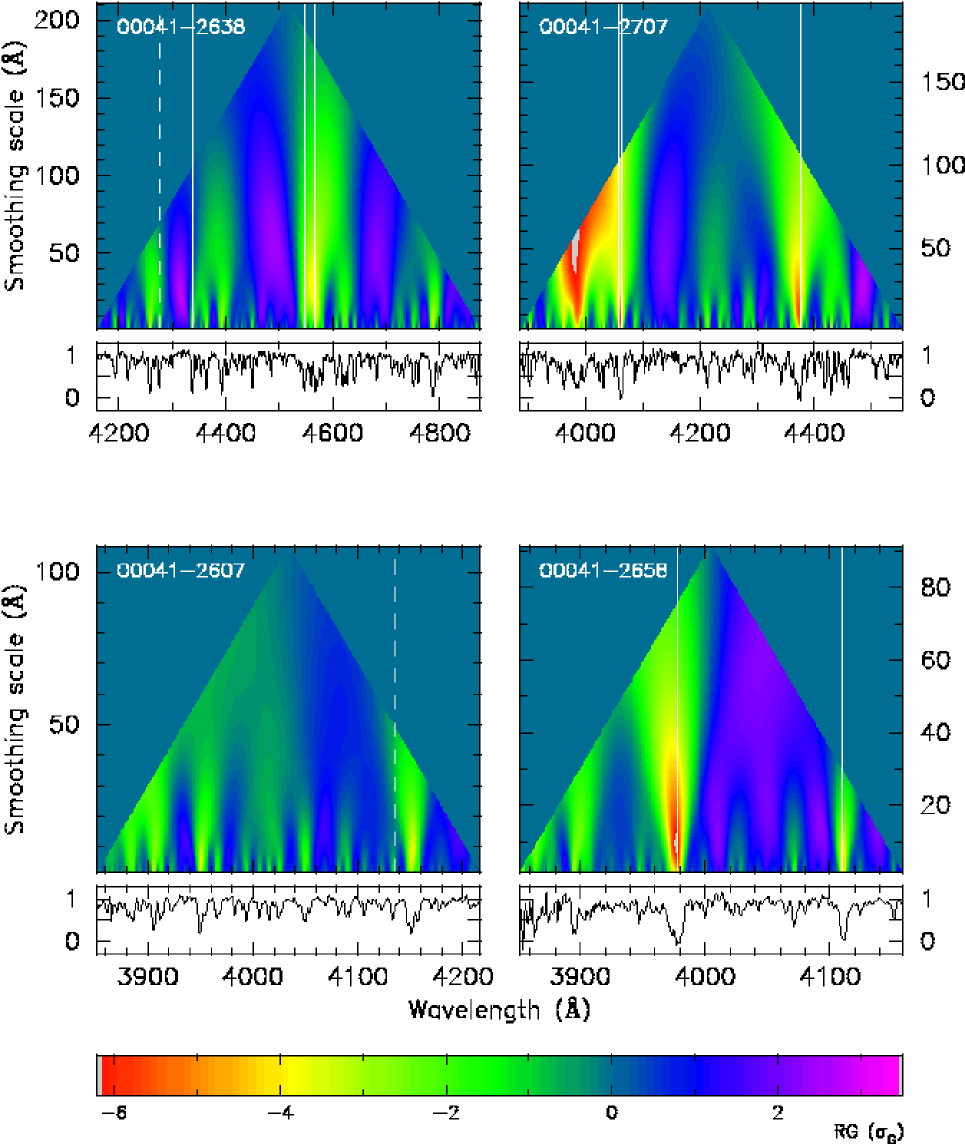
Figure 4: Reduced transmission triangles and normalised spectra of four of the QSOs listed in Table 2. The smoothing scale on the vertical axis is the FWHM of the smoothing Gaussian. Regions of overdense absorption appear yellow and red, underdense regions appear blue and purple. The vertical lines indicate the observed Ly$\alpha$ wavelengths of known metal absorption systems. Dashed lines mark the positions of metal systems that do not have an associated Ly$\alpha$ local minimum (see text).

In Fig. 4 we show the result of the analysis described above for four of the QSOs listed in Table 2 which show the most significant features as described below. The vertical lines show the Ly$\alpha$ positions of known metal systems which were primarily taken from ?) (their Table 3). A search using NED uncovered only three additional systems, all towards Q0042–2627 [York et al. (1991)]. Not surprisingly we see overdense Ly$\alpha$ absorption at the positions of all metal systems. We take this as an indication that our method correctly identifies overdensities.

Fig. 4 clearly demonstrates the presence of structures on scales as large as many hundred km s^-1. In all there are seven features which are significant at the more than $-4\sigma_{G}$ level. We now briefly describe these quite significant detections:

Q0041–2707: This spectrum shows three very significant overdensities in Ly$\alpha$. The first, $-6.2\sigma_{G}$ at $(\lambda,{\rm FWHM}_{\rm s})=(3983$ Å, $4179$ km s${}^{-1})$, is caused by an unsaturated cluster of lines which has no associated metal system. The second very significant ($-6.0\sigma_{G}$) overdensity in this spectrum lies at $(4062$ Å, $498$ km s${}^{-1})$ and is caused by a saturated blend. It seems to be associated with either or both of two metal systems detected in C IV and Si IV, Si II and C IV respectively. The third significant system is again associated with metals, is significant at the $-5.6\sigma_{G}$ level, and lies at $(4373$ Å, $745$ km s${}^{-1})$.

Q0041–2658: The most significant overdensity in the entire sample is a $-6.3\sigma_{G}$ overdensity at $(3977$ Å, $686$ km s${}^{-1})$, caused by a broad, clearly blended and saturated feature which is associated with C II, Si IV, C IV and Al II absorption. There is also a $-4.3\sigma_{G}$ overdensity at $(4111$ Å, $278$ km s${}^{-1})$, again associated with metals (S II and C IV).

Q0042–2627: A $-4.5\sigma_{G}$ overdensity at $(4522$ Å, $1071$ km s${}^{-1})$, with no associated metals, caused by a broad cluster of lines.

Q0043–2633: A $-5.2\sigma_{G}$ overdensity at $(4641$ Å, $778$ km s${}^{-1})$, with no associated metals, caused by a broad, saturated feature.

4.2 Local minima

The probability density function (pdf) of $G$ is inherently non-Gaussian, such that e.g. the probability of $G$ lying within $3\sigma_{G}$ of the mean is smaller than $0.9973$. In fact, the pdf of $G$ is a function of smoothing scale with the Central Limit Theorem guaranteeing a Normal distribution at very large smoothing scales. (We have attempted to continually remind the reader of this point by the persistent use of the notation ‘$\sigma_{G}$’.) In light of this difficulty it is necessary to estimate reliable significance levels by using simulated data.

To further demonstrate and quantify the significance of the overdensities presented in the previous section we investigate the statistics of local minima in the reduced transmission triangles by comparing them with the statistics of local minima derived from simulated data. We simply define a ‘local minimum’ (LM) as any pixel in a reduced transmission triangle with

$$RG(\lambda,\sigma_{\rm s})<-2.0\sigma_{G}$$ (7)

and where all surrounding pixels have larger values. If there is more than one LM in the same wavelength bin (but at different smoothing scales) then we delete the less significant one, since we do not want to count the same structure more than once. Given the resolution of the data it is evident that unclustered absorption lines will produce LM on the smallest smoothing scale ($=1.5$ Å). We may anticipate that the total number and distribution of these LM depend sensitively on the parameters of the underlying line distribution (1). Thus we exclude all LM on the smallest smoothing scale from all further analyses in order to reduce the model-dependence of our results.

Note that with this definition, almost all metal lines have a Ly$\alpha$ LM within $300$ km s^-1 (vertical lines in Fig. 4).

As mentioned in Section 3, we have simulated $100$ datasets ($=1000$ spectra), essentially by putting down Voigt profiles with parameters drawn from distribution (1) (see paper I for the exact technique). We then applied the same procedures as outlined above: first we constructed the reduced transmission triangles for all simulated spectra and then we determined the LM.

In the real data we found $103$ LM whereas the simulated data yielded on average $51$ LM with an rms dispersion of $7.6$. The maximum number of LM found in the $100$ simulated datasets was $70$. Thus there is an excess of the total number of LM over the expected number at the $>99$ per cent confidence level. In Fig. 6 we plot

$$\zeta(x)=\frac{N_{\rm obs}(x)}{N_{\rm exp}(x)}-1,$$ (8)

where $N_{\rm obs}$ ($N_{\rm exp}$) is the observed (expected, as derived from the simulations) number of LM and $x=RG$ (significance level of LM in units of $\sigma_{G}$) or $x={\rm FWHM}_{\rm s}$ (FWHM of smoothing Gaussian).

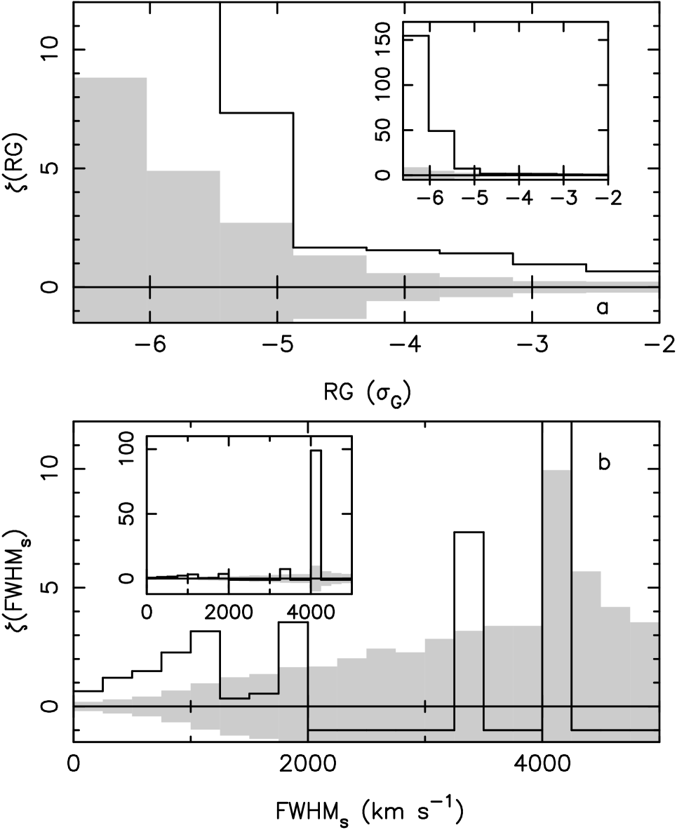
Figure 6: (a) Excess of observed number of local minima in reduced transmission triangles over the expected number ($=$ mean of $100$ simulations) as a function of the significance level of the local minima (see equation 8). $\pm 1$ rms levels as derived from the simulations are indicated by the grey shaded areas. (b) Same as (a) as a function of smoothing scale (FWHM of smoothing Gaussian). The insets show the same plots but with expanded $\zeta$-scales.

From panel (a) we can see that there is a tendency for the excess to be more significant for the stronger LM. For the leftmost bin we found two LM in the data but none in the $100$ simulated datasets. Extrapolating from lower significance levels we find $N_{\rm exp}=0.013$ for this bin, which is the value used in panel (a). A Kolmogorov–Smirnov test indicates that the distributions $N_{\rm obs}(RG)$ and $N_{\rm exp}(RG)$ disagree at the $95.6$ per cent confidence level. The excess is strengthened further and the confidence level is increased to $>99$ per cent by excluding all LM with smoothing scales $<250$ km s^-1 thus showing that the excess is dominated by the larger scale LM. In smoothing scale-space we also observe an excess which occurs on scales of up to $1200$ km s^-1 (panel b). By excluding LM with $RG>-4\sigma_{G}$, the excess on scales $<250$ km s^-1 disappears but it persists on larger scales thus showing that it is dominated by the more significant LM.

Q0041–2707 and Q0041–2658 exhibit the most significant structures, as can be seen in Fig. 4 (and as discussed in Section 4.1). If these two objects are removed from the sample the excess of LM is slightly reduced but remains significant at the $6.1\sigma$ level. The effect also persists if we exclude non-significant substructure from the analysis by deleting all LM which lie within the subtriangle defined by another more significant LM on larger smoothing scales. The removal of all LM that lie within $300$ km s^-1 of known metal lines again slightly weakens the excess of LM but does not remove the effect.

If we have used incorrect values for the observational parameters of equation (1) then we have over- or underestimated either the absolute value of the transmission fluctuations or their statistical significance or both. This may affect both the normalisation and the shape of the distributions $N_{\rm obs}(x)$. The exclusion of LM on the smallest smoothing scale from the analysis was designed to minimise the effect of changes of the above parameters on $N_{\rm exp}(x)$. We have checked the success of this strategy by creating six more sets of simulations, each consisting of $10$ datasets ($=100$ spectra). For each of these sets we varied one parameter: $\beta=1.7$, $\beta=1.3$, $B$ (overall normalisation) decreased and increased by $20$ per cent, $\mu_{b}=40$ km s^-1, and S/N $=10$. We have found no significant variation of the total number of LM in any of these simulations. The shapes of the distributions of LM as functions of $RG$ and FWHM_s also agree well with the distributions for the ‘standard’ case. The only exception was the $\beta=1.3$ model which produces less significant LM compared to the ‘standard’ case (although this has little effect on $\zeta(RG)$). In assessing the robustness of the result of Fig. 6 with respect to our choice of parameter values we thus only need to consider how the individual parameters affect $N_{\rm obs}$.

Given equation (5), $\sigma_{G}$ is virtually independent of $\gamma$ for all reasonable values. Thus the only effect of changing $\gamma$ is to change the size of the fluctuations, $G-\langle G\rangle$ in equation (6). Because we normalise $\langle G\rangle$ at the central wavelength of a spectrum (see equation 5) an increase in $\gamma$ will decrease the magnitude of overdensities at longer wavelengths while increasing the magnitude of overdensities at shorter wavelengths and vice versa. Thus there will only be an appreciable effect if overdensities tend to lie to one side of a spectrum which is not the case. In addition, a wrong $\gamma$ value cannot explain why the local minima occur almost exclusively on certain velocity scales. Nevertheless, we re-determined the LM for the real data for $\gamma=2.2$ and $\gamma=2.8$ and the effect is small.

By determining the normalisation of the effective optical depth for each spectrum individually we avoid over- or underestimation of $G-\langle G\rangle$ caused by small errors in the zeroth and first order of the continuum fits of the individual spectra. However, if the continua are systematically low or high then we will under- or overestimate the mean optical depth normalisation, $B$, and thus under- or overestimate $\sigma_{G}$. However, re-analysing the real data with $B$ increased by $20$ per cent we still find $98$ LM, significantly above the expected number of $51\pm 7.6$.

The parameters $\mu_{b}$, $\sigma_{b}$, and $b_{\rm cut}$ all affect the parameter $q$ in equation (3). ?) reported a possible evolution of $\mu_{b}$ with redshift over a range covered by the present data. If this were correct and if too small a value for $q$ were indeed the reason for the observed excess of LM then one would expect the excess to be larger at smaller redshifts where $\mu_{b}$ may be higher. Separating the data into a high and a low redshift bin we find $N_{\rm obs}(N_{\rm exp})=53(25\pm 5.0)$ and $50(26\pm 5.2)$ for the low and high redshift bins respectively. In any case, we have re-analysed the data for $\mu_{b}=40$ km s^-1 (which corresponds to an increase of $q$ of $\sim 30$ per cent, since $q$ is roughly linear in $\mu_{b}$) and still found $84$ LM.

Finally we have considered $\beta=1.3$ which also has the effect of increasing $\sigma_{G}$. A re-analysis of the data yielded $79$ LM which is still too large to be compatible with the simulations.

From the tests described above we conclude that the result presented in Fig. 6 is quite robust: there exist structures in the Ly$\alpha$ forest on scales of up to $\sim 1200$ km s^-1 at the $>99$ per cent confidence level. This result constitutes clear evidence for the non-uniformity of the Ly$\alpha$ forest on large scales despite repeated findings that the two-point correlation function of absorption lines shows no signal on scales $\mathrel{\mathchoice{\vbox{\offinterlineskip\halign{\hfil$\reset@font\displaystyle#$\hfil\cr>\cr\sim\cr}}}{\vbox{\offinterlineskip\halign{\hfil$\reset@font\textstyle#$\hfil\cr>\cr\sim\cr}}}{\vbox{\offinterlineskip\halign{\hfil$\reset@font\scriptstyle#$\hfil\cr>\cr\sim\cr}}}{\vbox{\offinterlineskip\halign{\hfil$\reset@font\scriptscriptstyle#$\hfil\cr>\cr\sim\cr}}}}300$ km s^-1 (e.g. [Cristiani et al. (1997)]).

4.3 Double lines of sight

Table 4: Pairs of QSOs grouped according to their proper transverse separation, $d$.

$d<3$ h-1 Mpc	$3$ h-1 Mpc $<d<6$ h-1 Mpc	$6$ h-1 Mpc $<d$
Q0041-2638 Q0042-2639	Q0041-2638 Q0042-2627	Q0041-2638 Q0041-2707
Q0041-2707 Q0041-2658	Q0041-2638 Q0042-2656	Q0041-2638 Q0041-2607
Q0042-2627 Q0042-2639	Q0041-2638 Q0043-2633	Q0041-2638 Q0042-2657
Q0042-2627 Q0043-2633	Q0041-2707 Q0042-2714	Q0041-2707 Q0041-2607
Q0042-2639 Q0043-2633	Q0041-2707 Q0042-2656	Q0041-2707 Q0042-2627
Q0042-2656 Q0042-2657	Q0041-2707 Q0042-2657	Q0041-2607 Q0041-2658
	Q0041-2607 Q0042-2627	Q0041-2607 Q0042-2714
	Q0041-2658 Q0042-2714	Q0041-2607 Q0042-2657
	Q0041-2658 Q0042-2657	Q0042-2627 Q0042-2656
	Q0042-2639 Q0042-2656	Q0042-2627 Q0042-2657
	Q0042-2639 Q0042-2657
	Q0042-2714 Q0042-2657
	Q0042-2656 Q0043-2633
	Q0042-2657 Q0043-2633
$\overline{d}=2.45$ h-1 Mpc	$\overline{d}=4.59$ h-1 Mpc	$\overline{d}=9.67$ h-1 Mpc

So far we have not taken advantage of the fact that the QSOs of Table 2 are a close group in the plane of the sky. We shall now examine possible correlations across lines of sight. One of the advantages of the analysis used above is that it is easily applied to multiple lines of sight: transmission triangles are simply averaged where they overlap. Given the transverse separations of the QSOs in this group and assuming reasonable absorber sizes, two different lines of sight will not probe the same absorbers. According to our null-hypothesis of an unclustered Ly$\alpha$ forest, two different lines of sight are therefore uncorrelated. Thus the variance of a mean transmission triangle (averaged over multiple lines of sight) is given by $\sigma_{G}^{2}(\lambda,\sigma_{\rm s})/n$, where $n$ is the number of triangles used at $(\lambda,\sigma_{\rm s})$. This procedure should enhance structures that extend across multiple lines of sight and surpress those that do not.

Here we present our results for the case $n=2$. We have sorted all pairs of QSOs into one of three groups according to the proper transverse separation, $d$, of the pair (calculated at the redshift of the lower redshift QSO): $d<3$ h^-1 Mpc, $3$ h^-1 Mpc $<d<6$ h^-1 Mpc and $6$ h^-1 Mpc $<d$. Table 4 lists those pairs within the groups for which the relevant spectral regions overlap.

As in Section 4.2 we proceeded to construct $\zeta$, but this time using only the overlap regions of the reduced mean triangles. Fig. 8 shows $\zeta(RG)$ and $\zeta({\rm FWHM}_{\rm s})$ for the three cases listed above. The top row shows the results for small transverse separations, the middle row for intermediate, and the bottom row for large transverse separations. There is evidence for a trend: with increasing separation we detect fewer and fewer overdensities at large significance levels and large smoothing scales relative to the simulations.

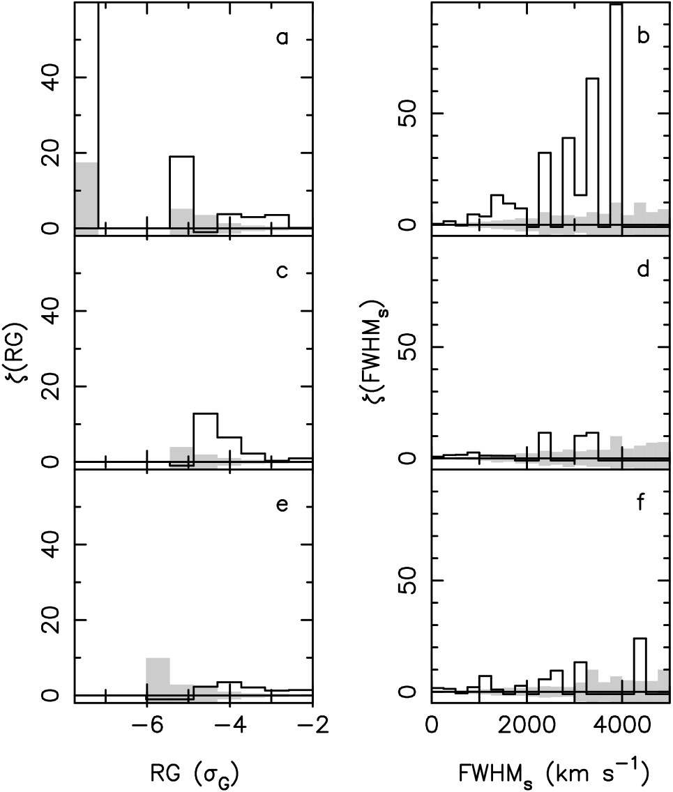
Figure 8: Excess of observed number of local minima in reduced mean transmission triangles of QSO pairs over the expected number ($=$ mean of $100$ simulations) as a function of the significance level (panels a, c, e) and the smoothing scale (panels b, d, f). The value of the leftmost bin of panel (a) is $303$. $\pm 1$ rms levels as derived from the simulations are indicated by the grey shaded areas. The top row shows the result for QSO pairs with $d<3$ h^-1 Mpc, the middle row for $3$ h^-1 Mpc $<d<6$ h^-1 Mpc and the bottom row for $6$ h^-1 Mpc $<d$.

In panel (a) there is an excess of LM which is somewhat weaker than that seen for single lines of sight (Fig. 6a). However, we detected one LM at $-7.5\sigma_{G}$. In contrast, the $100$ simulated datasets revealed no LM with $RG<-6\sigma_{G}$. (Extrapolating from lower significance levels gives $N_{\rm exp}=0.0033$ for this bin.) This very significant overdensity lies at $z=2.272$ and is produced by the near-coincidence in redshift space ($\Delta v\approx 450$ km s^-1) of the two most significant single-line of sight overdensities of the entire sample. These two overdensities are found in the spectra of Q0041–2658 and Q0041–2707. The two lines of sight are separated by $2.31$ h^-1 Mpc and are the second closest pair in the sample. This is a very clear example of a coherent structure traced by Ly$\alpha$ absorption extending across two lines of sight.

In all we detect $N_{\rm obs}(N_{\rm exp})=41(14\pm 4.7)$, $62(28\pm 6.9)$, and $65(25\pm 6.4)$ LM for small, intermediate, and large separations respectively. Thus the excess of the total number of LM does not seem to vary. However, the shapes of the distributions change quite significantly with line of sight separation. In Table 6 we list KS probabilities that the simulated and observed distributions of $RG$ values and smoothing scales agree for the three groups.

Table 6: Kolmogorov–Smirnov probabilities that the observed and expected distributions of $RG$ values and smoothing scales agree for the three line of sight separation groups.

	P${}_{\rm KS}(RG)$	P${}_{\rm KS}($FWHM${}_{\rm s})$
$d<3$:	$7\times 10^{-5}$	$8\times 10^{-5}$
$3<d<6$:	$0.011$	$0.017$
$6<d$:	$0.49$	$0.46$

At small separations, the simulated distributions disagree strongly with the observations, producing too few LM at large significance levels and at large smoothing scales. However at large separations, the distributions agree very well.

If the observed excess of LM in Figs 6 and 8(a) were simply due to an incorrect choice of the values for the parameters of equation (1) as discussed in Section 4.2, then it is hard to understand why that excess should be so strongly reduced for large line of sight separations. The removal of the pair Q0041–2707 - Q0041–2658 leaves the result qualitatively unchanged as does the removal of substructure as outlined in Section 4.2. The removal of all LM that have a metal system within $300$ km s^-1 in either of the spectra of the pair somewhat weakens the excess of panel (a) but does not remove the significance of the effect, since we still obtain P${}_{\rm KS}(RG)=9\times 10^{-4}$ and P${}_{\rm KS}($FWHM${}_{\rm s})=3\times 10^{-5}$ at small separations but good agreement at large separations (cf. Table 6).

A possible explanation for the trend of the decreasing excess with line of sight separation could be that the group of close QSO pairs is dominated by those QSOs whose spectra show the most significant overdensities and that these QSOs are absent from the group of large-separation pairs. However, by inspection of Table 4 we can see that each of the groups contains at least eight of the ten QSOs at least once. In particular, Q0041–2707 and Q0041–2658 are present in all groups and both appear in the group of close QSOs only once.

To further investigate whether the excess of LM seen in the double lines of sight (DLOS) is simply due to the excess already detected in the single lines of sight (SLOS) we attempt to identify the structures in the SLOS that give rise to the LM detected in the DLOS: for each LM in a DLOS we search for the most significant LM in each of the constituent SLOS within $1000$ km s^-1 (our results do not depend sensitively on this value). If the LM in the DLOS is due to a structure extending across the two lines of sight then one would expect less significant LM in both of the constituent SLOS. However, if the LM in the DLOS is due to a strong overdensity which does not extend across both SLOS then one would expect to find a LM in only one of the SLOS. If LM are found in both SLOS, then they may be quite dissimilar and one should be of greater significance than the LM in the DLOS. For each LM in the DLOS we have computed the following quantity:

• $\displaystyle\hskip 0.0pt{\frac{RG_{i}}{RG_{\rm D}}-1,\quad\quad i=1,2}$

where $RG_{i}$ denotes the LM in the two SLOS and $RG_{\rm D}$ that of the DLOS. This quantity measures how the SLOS-LM compare with the DLOS-LM they produce. In Fig. 10 we plot as thick solid lines the histograms of this measure for the three groups of QSO pairs (top = small separation, bottom = large separation). We have also computed the same histograms for the $100$ simulated datasets and display the mean and mean $\pm$ $1$ rms histograms as thin solid lines and grey shaded areas respectively. There is a small number of cases where no LM can be found in either of the single sight-lines and these are excluded from this analysis.

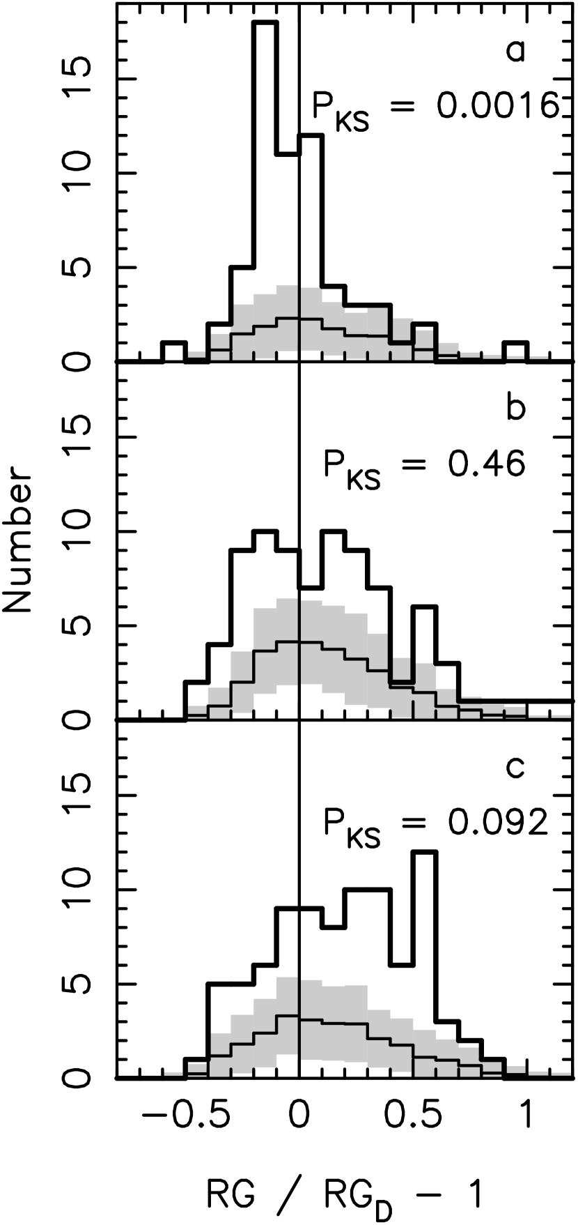
Figure 10: Histograms of the indicated quantity for all local minima detected in the reduced mean transmission triangles of QSO pairs (thick lines). The thin lines show the mean histograms computed from $100$ simulations. $\pm 1$ rms levels as derived from the simulations are indicated by the grey shaded areas. The top row shows the result for QSO pairs with $d<3$ h^-1 Mpc, the middle row for $3$ h^-1 Mpc $<d<6$ h^-1 Mpc and the bottom row for $6$ h^-1 Mpc $<d$. We also show KS probabilities that the simulated and observed distributions agree.

All panels of Fig. 10 show a large excess of the observed distributions over the simulated ones. This is not overly surprising since we already know that the total number of LM exceeds the expected number at all separations. However, at small separations (panel a) the excess is skewed to values $RG/RG_{\rm D}-1<0$. A KS test shows that the simulated and observed distributions disagree at the $>99$ per cent confidence level. This discrepancy disappears for larger line of sight separations.

In addition, we have also counted the number of DLOS-LM which are produced by only a single SLOS-LM and found that the excess of such cases increases from $2.2\sigma$ over $3.4\sigma$ to $4.4\sigma$ for increasing line of sight separation.

Again, the removal of certain subclasses of LM (those of the Q0041–2707 - Q0041–2658 pair, substructure, those associated with metal lines) does not change the results significantly.

In summary, the results above show that for small line of sight separations two SLOS-LM combine to make a DLOS-LM of greater significance, whereas for large line of sight separations the structures seen in the SLOS are ‘diluted’. We thus take the anti-correlation of the excess of LM seen in the reduced mean transmission triangles of double-lines of sight with sight-line separation as strong evidence for the existence of structures on scales of up to $3$ h^-1 proper Mpc in the Ly$\alpha$ forest.

4.4 Correlation with metal lines

Not surprisingly, all the metal systems that were found in the present data have associated overdense Ly$\alpha$ absorption. We have repeatedly remarked in the sections above that the removal of LM that are associated with metal lines does not change the results qualitatively. Here, we take the opposite approach: we have repeated the analysis of the previous section only for those DLOS-LM that have a metal system within $1000$ km s^-1 in either of the constituent SLOS. The corresponding figure to Fig. 8 shows only a marginal trend with line of sight separation, with P${}_{\rm KS}(RG)=0.091$ for small separations, which is entirely due to the close pair Q0041–2658 and Q0041–2707. The corresponding figure to Fig. 10 and its KS tests also indicate that the DLOS-LM are due to chance alignments or single SLOS-LM at all separations, however the numbers are very low and we cannot draw any definite conclusions.

It must be kept in mind that the subdivision into LM with and without metals is subject to a strong selection effect since the work by ?) and ?) has clearly shown that the census of C IV in the present data must be significantly incomplete. Thus the distinction made here is more one between high-column density vs. low-column density structures rather than between metals vs. Ly$\alpha$ only. Therefore in the real data we have selected LM that are due to high-column density structures whereas in the simulations we have basically drawn a random sample of LM since in the simulated data the column density is unrelated to the presence of metals.

Nevertheless, it appears that the high-column density structures traced by metal lines do not produce overdense Ly$\alpha$ absorption at the distances probed by this sample, with one notable exception, in contrast to the lower column density Ly$\alpha$ only systems. On the other hand, there is little difference between the distributions of smoothing scales for those LM that are associated with metal lines and those that are not. A KS test gives a probability of $0.3$ that the two distributions are the same.

4.5 Triple lines of sight

Table 8: Triplets of QSOs grouped according to their proper transverse separation, $d$.

$d<3$ h-1 Mpc	$3$ h-1 Mpc $<d<6$ h-1 Mpc	$6$ h-1 Mpc $<d$
Q0042-2627 Q0042-2639 Q0043-2633	Q0041-2638 Q0042-2656 Q0043-2633	Q0041-2638 Q0041-2707 Q0041-2607
	Q0041-2707 Q0042-2714 Q0042-2657	Q0041-2638 Q0041-2607 Q0042-2657
	Q0041-2658 Q0042-2714 Q0042-2657
$\overline{d}=2.82$ h-1 Mpc	$\overline{d}=4.73$ h-1 Mpc	$\overline{d}=8.92$ h-1 Mpc

QSO triplets can provide important constraints on the shape of Ly$\alpha$ absorbers. It is possible that the excess of LM seen in the DLOS is mainly due to filamentary structures. If this were the case then one would expect LM of close triple lines of sight (TLOS) to be caused by two, not three SLOS-LM. However, if the absorption is sheet-like in nature then one would expect to find three similar SLOS-LM per TLOS-LM.

We have repeated the analysis of Section 4.3 for triple lines of sight. Table 8 lists triplets of QSOs grouped according to their pairwise transverse line of sight separations as in Table 4. The triplets of the first two groups form more or less equilateral triangles on the sky. However, due to the larger extent of the full group in the DEC direction than in the RA direction, the triplets of the last group form somewhat flatter triangles. Unfortunately, our QSO sample is not dense enough to provide more than one to three triplets per group.

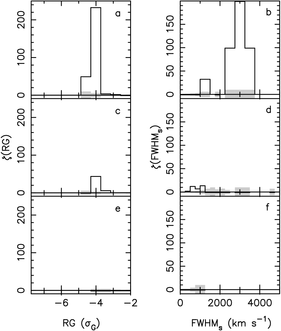
Figure 12: Excess of observed number of local minima in reduced mean transmission triangles of QSO triplets over the expected number ($=$ mean of $100$ simulations) as a function of the significance level (panels a, c, e) and the smoothing scale (panels b, d, f). $\pm 1$ rms levels as derived from the simulations are indicated by the grey shaded areas. The top row shows the result for QSO triplets with pairwise separations $d<3$ h^-1 Mpc, the middle row for $3$ h^-1 Mpc $<d<6$ h^-1 Mpc and the bottom row for $6$ h^-1 Mpc $<d$.

Fig. 12 shows the results. Again we see an anti-correlation of the excess of LM with line of sight separation (panels a, c, and e). However, for the smallest separations we find that $7$ of the $10$ identified TLOS-LM are due to only two (and not three) SLOS-LM. The vast majority of SLOS-LM are of smaller significance than their respective TLOS-LM. Therefore it seems that at least in the case of this particular QSO triplet the absorption more often extends across only two lines of sight than across three. However, the numbers are small and thus we cannot draw any definite conclusions from this result.

5 Conclusions and discussion

We summarise our main results as follows:

(1) We have analysed the Ly$\alpha$ forest spectra of ten QSOs at $\langle z\rangle=2.81$ contained within a $\sim 1$ deg² field using a new technique based on the statistics of the transmitted flux. Comparison with two-point correlation function analyses (Section 4.2), along with the results of paper I, suggests that this new method is more sensitive to the presence of large-scale structure than the two-point correlation function of individually identified absorption lines.

(2) We find structure on scales of up to $1200$ km s^-1 along the line of sight and on scales of up to $17$ h^-1 Mpc (comoving) in the transverse direction. We confirm the existence of large-scale structure in the Ly$\alpha$ forest at the $>99$ per cent confidence level ([Pando & Fang (1996)]; [Williger et al. (1999)]).

(3) We find strong correlations across lines of sight with proper separation $<3$ h^-1 Mpc. For intermediate separations the correlation is weaker and there is only little evidence for correlation at line of sight separations $>6$ h^-1 Mpc (Fig. 8). We thus present the first evidence for a dependence of the correlation strength on line of sight separation, and place an upper limit of $6$ h^-1 Mpc on the transverse correlation scale at $z=2.81$.

Assuming that the absorbing structures are expanding with the Hubble flow, we find that the line of sight and transverse correlation scales are roughly comparable ($1200$ km s${}^{-1}H^{-1}(z=2.81)=1.6$ h^-1 Mpc) with a suggestion that the absorbers might be flattened in the line of sight direction since we still detect somewhat significant correlations on transverse scales of $4.6$ h^-1 Mpc. Furthermore, the analysis of the only close QSO triplet of the sample showed that many coincident absorption features are common to only two spectra, perhaps indicating an elongated shape in the plane of the sky. However, no firm conclusions can be drawn here until more QSO triplets have been analysed.

Using a comparatively small sample with significantly smaller line of sight separations, ?) and ?) found a stronger correlation signal for lines with $W>0.4$ Å than for weaker lines. In contrast, ?) found from their analysis of the present SGP data that the inclusion of weak lines ($W>0.1$ Å) strengthened their correlation signal. Here we can tentatively confirm the ?) result. This is in agreement with the results of ?) who predicted from their numerical simulations that high-column density lines have smaller correlation lengths than low-column density ones. This is already evident from a visual inspection of the three-dimensional distribution of the absorbing gas in the simulations at different overdensities. Large overdensities are confined to relatively small, more or less spherical regions whereas small overdensities form extended filaments and sheets.

It is interesting to compare our results with predictions from hydrodynamical simulations. The typical length of the low-column density filaments in the simulations is of the order of $1$ h^-1 Mpc in proper units ([Miralda-Escudé et al. (1996)]; [Zhang et al. (1998)]). ?) performed a detailed analysis of double-lines of sight in a $\Lambda$CDM simulation. They concluded that for proper line of sight separations $>500$ h^-1 kpc any coincident absorption is due to unrelated and spatially uncorrelated clouds. They pointed out however that a significant amount of power is missing from their simulation on the scale of the simulated box size ($10$ h^-1 Mpc). Even after correcting for this effect though, the transverse correlation scale predicted from these simulations remains significantly smaller (by about a factor of $3$) than the one derived in this work. To investigate this discrepancy it will be necessary to perform a detailed comparison by subjecting simulated spectra, drawn from a suitable (i.e. large) simulation box, to the same analysis we have presented here.

?) and ?) have outlined schemes for recovering the power spectrum of mass fluctuations from Ly$\alpha$ forest spectra. Recently, ?) performed the first such measurement on scales of $2$–$12$ h^-1 Mpc from $19$ intermediate-resolution QSO spectra at $z=2.5$. Although we have concentrated in this work only on identifying typical correlation scales, our results confirm the usefulness of intermediate-resolution data for large-scale structure studies when analysing the distribution of the transmitted flux directly. Since the Ly$\alpha$ forest is thought to trace the mass distribution more closely than galaxies we are likely to gain the most direct measurement of the bias between galaxy and mass clustering by comparing the power spectrum of the Ly$\alpha$ forest with that of galaxies [Croft et al. (1998b)].

References

- Bahcall et al. (1991) Bahcall J. N., Jannuzi B. T., Schneider D. P., Hartig G. F., Bohlin R., Junkkarinen V., 1991, ApJ, 377, L5
- Bi & Davidsen (1997) Bi H., Davidsen A. F., 1997, ApJ, 479, 523
- Bowen et al. (1996) Bowen D. V., Blades J. C., Pettini M., 1996, ApJ, 464, 141
- Carswell et al. (1984) Carswell R. F., Morton D. C., Smith M. G., Stockton A. N., Turnshek D. A., Weymann R. J., 1984, ApJ, 278, 486
- Cen et al. (1994) Cen R., Miralda-Escudé J., Ostriker J. P., Rauch M., 1994, ApJ, 437, L9
- Cen & Simcoe (1997) Cen R., Simcoe R. A., 1997, ApJ, 483, 8
- Charlton et al. (1995) Charlton J. C., Churchill C. W., Linder S. M., 1995, ApJ, 452, L81
- Chen et al. (1998) Chen H.-W., Lanzetta K. M., Webb J. K., Barcons X., 1998, ApJ, 498, 77
- Chernomordik (1995) Chernomordik V. V., 1995, ApJ, 440, 431
- Cowie et al. (1995) Cowie L. L., Songaila A., Kim T.-S., Hu E. M., 1995, AJ, 109, 1522
- Cristiani et al. (1997) Cristiani S., D’Odorico S., D’Odorico V., Fontana A., Giallongo E., Savaglio S., 1997, MNRAS, 285, 209
- Cristiani et al. (1995) Cristiani S., D’Odorico S., Fontana A., Giallongo E., Savaglio S., 1995, MNRAS, 273, 1016
- Croft et al. (1998a) Croft R. A. C., Weinberg D. H., Katz N., Hernquist L., 1998a, ApJ, 495, 44
- Croft et al. (1998b) Croft R. A. C., Weinberg D. H., Pettini M., Hernquist L., Katz N., 1998b, ApJ, submitted, astro-ph/9809401
- Crotts (1989) Crotts A. P. S., 1989, ApJ, 336, 550
- Crotts & Fang (1998) Crotts A. P. S., Fang Y., 1998, ApJ, 502, 16
- Davé et al. (1998a) Davé R., Hellsten U., Hernquist L., Katz N., Weinberg D. H., 1998a, ApJ, 509, 661
- Davé et al. (1998b) Davé R., Hernquist L., Katz N., Weinberg D. H., 1998b, ApJ, 511, 521
- Davé et al. (1997) Davé R., Hernquist L., Weinberg D. H., Katz N., 1997, ApJ, 477, 21
- Dinshaw et al. (1998) Dinshaw N., Foltz C. B., Impey C. D., Weyman R. J., 1998, ApJ, 494, 567
- Dinshaw et al. (1997) Dinshaw N., Weyman R. J., Impey C. D., Foltz C. B., Morris S. L., Ake T., 1997, ApJ, 491, 45
- D’Odorico et al. (1998) D’Odorico V., Cristiani S., D’Odorico S., Fontana A., Giallongo E., Shaver P., 1998, A&A, 339, 678
- Elowitz et al. (1995) Elowitz R. M., Green R. F., Impey C. D., 1995, ApJ, 440, 458
- Fang et al. (1996) Fang Y., Duncan R. C., Crotts A. P. S., Bechtold J., 1996, ApJ, 462, 77
- Fernández-Soto et al. (1996) Fernández-Soto A., Lanzetta K. M., Barcons X., Carswell R. F., Webb J. K., Yahil A., 1996, ApJ, 460, L85
- Gnedin (1998) Gnedin N. Y., 1998, MNRAS, 294, 407
- Gnedin & Hui (1998) Gnedin N. Y., Hui L., 1998, MNRAS, 296, 44
- Hernquist et al. (1996) Hernquist L., Katz N., Weinberg D. H., Miralda-Escudé J., 1996, ApJ, 457, L51
- Hu et al. (1995) Hu E. M., Kim T.-S., Cowie L. L., Songaila A., Rauch M., 1995, AJ, 110, 1526
- Hui et al. (1997) Hui L., Gnedin N. Y., Zhang Y., 1997, ApJ, 486, 599
- Ikeuchi (1986) Ikeuchi S., 1986, ApJS, 118, 509
- Ikeuchi & Ostriker (1986) Ikeuchi S., Ostriker J. P., 1986, ApJ, 301, 522
- Khare et al. (1997) Khare P., Srianand R., York D. G., Green R., Welty D., Huang K.-L., Bechtold J., 1997, MNRAS, 285, 167
- Kim et al. (1997) Kim T.-S., Hu E. M., Cowie L. L., Songaila A., 1997, AJ, 114, 1
- Kirkman & Tytler (1997) Kirkman D., Tytler D., 1997, ApJ, 484, 672
- Kulkarni et al. (1996) Kulkarni V. P., Huang K., Green R. F., Bechtold J., Welty D. E., York D. G., 1996, MNRAS, 279, 197
- Lanzetta et al. (1995) Lanzetta K. M., Bowen D. B., Tytler D., Webb J. K., 1995, ApJ, 442, 538
- Le Brun & Bergeron (1998) Le Brun V., Bergeron J., 1998, A&A, 332, 814
- Le Brun et al. (1996) Le Brun V., Bergeron J., Boissé P., 1996, A&A, 306, 691
- Liske et al. (1998) Liske J., Webb J. K., Carswell R. F., 1998, MNRAS, 301, 787
- Lu et al. (1998) Lu L., Sargent W. L. W., Barlow T. A., Rauch M., 1998, AJ, submitted, astro-ph/9802189
- Lu et al. (1996) Lu L., Sargent W. L. W., Womble D. S., Takada-Hidai M., 1996, ApJ, 472, 509
- Meiksin & Bouchet (1996) Meiksin A., Bouchet F. R., 1996, MNRAS, 283, 1388
- Miralda-Escudé et al. (1996) Miralda-Escudé J., Cen R., Ostriker J. P., Rauch M., 1996, ApJ, 471, 582
- Miralda-Escudé & Rees (1997) Miralda-Escudé J., Rees M. J., 1997, ApJ, 478, L57
- Mo et al. (1992) Mo H. J., Xia X. Y., Deng Z. G., Börner G., Fang L. Z., 1992, A&A, 256, L23
- Morris et al. (1991) Morris S. L., Weymann R. J., Savage B. D., Gilliland R. L., 1991, ApJ, 377, L21
- Mücket et al. (1996) Mücket J. P., Petitjean P., Kates R. E., Riediger R., 1996, A&A, 308, 17
- Nusser & Haehnelt (1999) Nusser A., Haehnelt M., 1999, MNRAS, 303, 179
- Oke & Korycansky (1982) Oke J. B., Korycansky D. G., 1982, ApJ, 255, 11
- Ostriker et al. (1988) Ostriker J. P., Bajtlik S., Duncan R. C., 1988, ApJ, 327, L35
- Ostriker & Ikeuchi (1983) Ostriker J. P., Ikeuchi S., 1983, ApJ, 268, L63
- Pando & Fang (1996) Pando J., Fang L.-Z., 1996, ApJ, 459, 1
- Pando & Fang (1998) Pando J., Fang L.-Z., 1998, A&A, 340, 335
- Petitjean et al. (1995) Petitjean P., Mücket J. P., Kates R. E., 1995, A&A, 295, L9
- Petitjean et al. (1998) Petitjean P., Surdej J., Smette A., Shaver P., Mücket J., Remy M., 1998, A&A, 334, L45
- Rauch & Haehnelt (1995) Rauch M., Haehnelt M. G., 1995, MNRAS, 275, 76
- Rees (1986) Rees M. J., 1986, MNRAS, 218, 25
- Riediger et al. (1998) Riediger R., Petitjean P., Mücket J. P., 1998, A&A, 329, 30
- Sargent et al. (1980) Sargent W. L. W., Young P. J., Boksenberg A., Tytler D., 1980, ApJS, 42, 41
- Smette et al. (1995) Smette A., Robertson J. G., Shaver P. A., Reimers D., Wisotzki L., Köhler T., 1995, A&AS, 113, 199
- Songaila & Cowie (1996) Songaila A., Cowie L. L., 1996, AJ, 112, 335
- Theuns et al. (1998) Theuns T., Leonard A., Efstathiou G., 1998, MNRAS, 297, L49
- Theuns et al. (1998) Theuns T., Leonard A., Efstathiou G., Pearce F. R., Thomas P. A., 1998, MNRAS, 301, 478
- Tripp et al. (1998) Tripp T. M., Lu L., Savage B. D., 1998, ApJ, 508, 200
- Ulmer (1996) Ulmer A., 1996, ApJ, 473, 110
- Wadsley & Bond (1997) Wadsley J. W., Bond J. R., 1997, in ASP Conference Series, Vol. 123, Clarke D. A., West M. J., ed, Proceedings of the 12th Kingston Meeting “Computational Astrophysics”, San Francisco, p. 332, astro-ph/9612148
- Webb (1987) Webb J. K., 1987, in Hewitt A., Burbidge G., Fang L.-Z., ed, Proceedings of the 124th IAU Symposium “Observational Cosmology”. Reidel, Dordrecht, p. 803
- Webb et al. (1992) Webb J. K., Barcons X., Carswell R. F., Parnell H. C., 1992, MNRAS, 255, 319
- Williger & Babul (1992) Williger G. M., Babul A., 1992, ApJ, 399, 385
- Williger et al. (1996) Williger G. M., Hazard C., Baldwin J. A., McMahon R. G., 1996, ApJS, 104, 145
- Williger et al. (1999) Williger G. M., Smette A., Hazard C., Baldwin J. A., McMahon R. G., 1999, ApJ, in press, astro-ph/9910369
- York et al. (1991) York D. G., Yanny B., Crotts A., Carilli C., Garrison E., 1991, MNRAS, 250, 24
- Zhang et al. (1995) Zhang Y., Anninos P., Norman M. L., 1995, ApJ, 453, L57
- Zhang et al. (1997) Zhang Y., Anninos P., Norman M. L., Meiksin A., 1997, ApJ, 485, 496
- Zhang et al. (1998) Zhang Y., Meiksin A., Anninos P., Norman M. L., 1998, ApJ, 495, 63