Evidence for Large Scale Structure in the Ly$\alpha$ Forest at $z>2.6$

Abstract

We present a search for spatial and redshift correlations in a 2 Å resolution spectroscopic survey of the Ly$\alpha$ forest at $2.15<z<3.37$ toward ten QSOs concentrated within a 1^∘ diameter field. We find a signal at $2.7\sigma$ significance for correlations of the Ly$\alpha$ absorption line wavelengths between different lines of sight over the whole redshift range. The significance rises to $3.2\sigma$ if we restrict the redshift range to $2.60<z<3.37$, and to $4.0\sigma$ if we further restrict the sample to lines with rest equivalent width $0.1\leq W_{0}/{\rm\AA}<0.9$. We conclude that a significant fraction of the Ly$\alpha$ forest arises in structures whose correlation length extends at least over 30 arcmin ($\sim 26~{}h^{-1}$ comoving Mpc at $z=2.6$ for $H_{0}\equiv 100h$ km s^-1 Mpc^-1, $\Omega=1.0$, $\Lambda=0$). We have also calculated the three dimensional two point correlation function for Ly$\alpha$ absorbers; we do not detect any significant signal in the data. However, we note that line blending prevents us from detecting the signal produced by a 100% overdensity of Ly$\alpha$ absorbers in simulated data. We find that the Ly$\alpha$ forest redshift distribution provides a more sensitive test for such clustering than the three dimensional two point correlation function.

1 Introduction

Much progress has been made in understanding the origin of the numerous narrow Ly$\alpha$ absorption lines observed in quasar spectra since their discovery ([38]). Their large number density along a typical line of sight ([58]) shows a strong evolution with redshift, outnumbering any other known object ([37]; [1]) for redshifts accessible from the ground ($z>1.6$). Comparison between spectra for each component of multiply lensed quasars ([26]; [60], 1995) or close quasar pairs ( [2]; [18], 1995, 1997; [24]; [23]; [54]) indicate that they are produced in large tenuous clouds with diameters exceeding 50 $h^{-1}$ kpc ($H_{0}\equiv 100h$ km s^-1 Mpc^-1). The high signal to noise ratio spectra obtained with the 10m Keck telescope have revealed the presence of C iv absorption lines associated with 75% of the lines with column densities $N_{\rm HI}>3~{}10^{14}{\rm cm}^{-2}$ and 90% of the ones with $N_{\rm HI}>1.6~{}10^{15}{\rm cm}^{-2}$ ([62]). Furthermore, the lines with $N_{\rm HI}>1.6~{}10^{15}{\rm cm}^{-2}$ show only an order of magnitude range in ionization ratios. These observations indicate that, although of low metallicities, these clouds are not made of pristine material, which in turn suggests the existence of a very first generation of massive stars contaminating the intergalactic medium with heavy elements ([42]) as they turned supernovae.

A possible association with galaxies which could also explain their metal content as processed gas is unclear ([44]; [45]; [43]; [34]; [5]; [35]; [64]; [57]; [9]; [63]; [27]; [30]). At low redshift, where the detection of galaxies is fairly complete to low-luminosity, a consensus appears that the largest column density Ly$\alpha$ systems are distributed more like galaxies than the low column density ones ($\log N_{HI}\mathrel{\hbox to0.0pt{\lower 3.0pt\hbox{$\mathchar 536\relax$}\hss}\raise 2.0pt\hbox{$\mathchar 316\relax$}}14-15$ or rest equivalent width $W_{0}\mathrel{\hbox to0.0pt{\lower 3.0pt\hbox{$\mathchar 536\relax$}\hss}\raise 2.0pt\hbox{$\mathchar 318\relax$}}0.1-0.3$ Å; see [59]).

There is evidence that lower column density systems also correlate with galaxies ([63]; [30]), though Impey et al. found that it is not possible to assign uniquely a galaxy counterpart to an absorber, and that there is no support for absorbers to be located preferentially with the haloes of luminous galaxies. Extrapolations of these Ly$\alpha$ cloud-galaxy correlations to $z\sim 2-3$ (in the general context of galaxy and density perturbation distributions) are consistent with observed Ly$\alpha$ cloud clustering properties, which have only revealed signals on very small velocity scales ([66]; [11], 1997; [40]; [10]; [62]; [25]).

There has been much effort made to examine the two point correlation function at $z>1.6$ in the Ly$\alpha$ forest along isolated lines of sight, with some contradictory results. On one side, Cristiani et al. (1997) found a 5$\sigma$ detection at $\Delta v<300$ km s^-1 and Khare et al. (1997) detected a $>3\sigma$ signal at $\Delta v=50-100$ km s^-1, based on 4m-class telescope echelle spectra, and Kim et al. (1997) presented a $2.5-2.8\sigma$ significance signal at $\Delta v=75$ km s^-1 based on 10m Keck–HIRES data. On the other, Kirkman & Tytler (1997) failed to confirm such claims with high signal to noise ratio Keck–HIRES spectra.

A complementary approach is to examine structure between adjacent lines of sight. For the Ly$\alpha$ forest on small scales, Crotts (1989) and Crotts & Fang (1998) searched for spatial structure in the Ly$\alpha$ forest at $z<2.6$ on angular scales of $2\mathrel{\hbox to0.0pt{\lower 3.0pt\hbox{$\mathchar 536\relax$}\hss}\raise 2.0pt\hbox{$\mathchar 316\relax$}}\Delta\theta/{\rm arcmin}\mathrel{\hbox to0.0pt{\lower 3.0pt\hbox{$\mathchar 536\relax$}\hss}\raise 2.0pt\hbox{$\mathchar 316\relax$}}3$ separation. They found that the two point correlation function presents an excess for velocity separations of $\Delta v\approx 200$ km s^-1 for $W_{0}\geq 0.4$ Å absorbers, with a tentative conclusion that $W_{0}\geq 0.4$ Å absorbers are sheet-like. Their results indicate the existence of coherent structure on scales $\sim 0.7~{}h^{-1}~{}$ comoving Mpc at $z>2$. At lower redshift, Dinshaw et al. (1995) found evidence of clustering on the scale of 100 km s^-1 at $0.5<z<0.9$ over a separation of $\Delta\theta=1.4$ arcmin ($\sim 350h^{-1}$ kpc), though it is not clear whether this scale probes the same clouds or is more characteristic of a correlation length. Theoretically, McDonald & Miralda-Escudé (1999) calculated the correlation function in three dimensions for the Ly$\alpha$ forest between lines of sight separated by $\Delta\theta\leq 5$ arcmin, suggesting that such a method could be used to measure cosmological parameters ($\Omega_{0}$, $\Omega_{\Lambda}$).

On larger scales, correlated C iv absorption between lines of sight separated by several tens of arcmin has already revealed structures on the scale of several Mpc ([65], hereafter Paper I; [20]). A marginal correlation in the Ly$\alpha$ forest has been suggested on the $1^{\circ}$ scale ([55]). Otherwise, Ly$\alpha$ forest correlations on large angular scales have remained largely unexplored.

A parallel analysis of the same south Galactic pole spectra as used here was carried out by Liske et al. (1999). It uses a new method to study correlations based on the statistics of transmitted flux. Their results reveal the C iv cluster at $z\sim 2.3$ which was found in Paper I, as well as a void toward four lines of sight at least $36\times 24h^{-2}$ comoving Mpc² in extent at $z=2.97$ at the $4\sigma$ significance level. The void happens to coincide with the location of a nearby QSO.

On the theoretical side, several recent N-body simulations performed in boxes of $10-20h^{-1}$ comoving Mpc ([6]; [52]; [28]; [46]; [7]; [67], 1998; [16]) and an analytical study ([3]) suggest that Ly$\alpha$ clouds are associated with filaments or large, flattened structures, similar to Zel’dovich pancakes, associated with low overdensity of the dark matter distribution ($\delta\rho/\langle\rho\rangle<30$). Such structures may be detectable as correlations in the Ly$\alpha$ forest toward groups of adjacent QSOs. Detailed analyses for the observable effects of such $\sim 30h^{-1}$ comoving Mpc scale structures toward groups of QSOs on the sky have not been performed, though much smaller scales ($\leq 0.56h^{-1}$ comoving Mpc) have been considered ([8]).

In this paper, the Ly$\alpha$ forest toward ten $2.36<z<3.44$ QSOs concentrated within a $1^{\circ}$ diameter field near the SGP is used as a probe for the existence of $\sim 30h^{-1}$ comoving Mpc scale structures transverse to the lines of sight. In §2, we review the observational data used in the analysis. In §3, we describe the statistical tests made, and the results we obtained. We discuss the implications of the correlations we find in §4. Throughout this paper, we assume $\Omega=1.0$ and $\Lambda=0$.

2 The Data

The observational data consist of the 10 highest signal to noise ratio spectra covering the Ly-$\alpha$ forest that were obtained during a parallel study (Paper I) on the large scale structure revealed by C IV absorbers, in front of 25 QSOs at $z>2$ within a $\simeq 1^{\circ}$ diameter field. The location of the QSOs on the sky and details of the observations and reductions are presented in Paper I. The instrumental resolution was $\sim 2$ Å, which allows us to resolve lines with a velocity difference of $\Delta v>140$ km s^-1 at $z=3$. The signal to noise ratio per 1 Å pixel reaches up to 40 between the Ly$\alpha$ and Ly $\beta$ emission lines. Further details of the observations and reductions are given in Paper I. We stress the homogeneity of the instrumental set-up, of the reduction process and of the line list preparation procedures. The mean 1$\sigma$ uncertainty in wavelength centroids is $\sigma_{v}=13$ km s^-1.

The sample used for the analysis contains all the Ly$\alpha$ lines with rest equivalent widths $W_{\rm 0}>0.1$ Å detected at the 5$\sigma$ significance level and which lie between the Ly$\alpha$ and Ly$\beta$ emission line wavelengths. However, we have excluded lines that belong to known metal absorbers (cf. Paper I) or lie within $5000$ km s^-1 from the background QSO. The latter condition has been set to avoid uncertainties introduced by the “proximity effect” (which reduces the line number density and the equivalent widths of the lines). The line sample is thus a subset taken from Table 2 of Paper I, and consists of 383 Ly$\alpha$ lines at $2.15<z<3.26$. However, we note that completeness is only reached over the whole set of spectra for lines with $W_{0}=0.5$ Å. It is now generally accepted that there are very few Ly-$\alpha$ lines with $b<18$ km s^-1 lines ([29]; [33]). Consequently, all lines with $W_{0}\geq 0.1$ Å observed here have $\log N_{\rm HI}/{\rm cm}^{-2}>13.4$. Figure 1 presents the locations and rest equivalent widths of the absorbers projected onto the right ascension and declination planes.

Figure 1: Above:  Solid lines show the redshift coverage for Ly$\alpha$ in the QSO data in the sample, projected onto the declination plane and centered at right ascension $\alpha=0^{\rm h}44^{\rm m}42\hbox to0.0pt{$.$\hss}^{\rm s}15$ (J2000). Open stars indicate QSOs used in the sample from Paper I, with their names being listed adjacent. Spectral regions within $5000$ km s^-1 from the background QSOs are not used, to discard absorption systems possibly affected by the proximity effect. Absorption lines with $W_{0}\geq 0.1$ Å at $\geq 5\sigma$ detection significance were used in the analysis, and are shown as ticks whose length is proportional to $W_{0}$. Absorbers corresponding to known metal systems from the C iv survey have been omitted. Below:  Same as above, except projected onto the right ascension plane and centered at declination $\delta=-27^{\circ}25^{\prime}06^{\prime\prime}$ (J2000).

Each individual line of sight shows no unusual distribution of absorption systems with redshift or rest equivalent width. We used the program SEWAGE (Sophisticated and Efficient $W^{*}$ And Gamma Estimator), kindly provided to us by Dobrzycki (1999). The redshift number density of $W_{0}\geq 0.5$ Å lines is consistent with a power law distribution ([37]) $d{\cal N}/dz\propto(1+z)^{\gamma}$, with a maximum likelihood value $\gamma=2.02\pm 1.24$. The corresponding rest equivalent width distribution is consistent with $d{\cal N}/dW\propto e^{-W/W^{*}}$, $W^{*}=0.43\pm 0.04$. We find no large voids in any line sample defined by a minimum rest equivalent width, following the method described in Ostriker, Bajtlik, & Duncan (1988).

The instrumental resolution of $\sim 2$ Å makes the minimum detected separation in a single spectrum between lines of strongly different strengths to be $\sim 3.7$Å, which corresponds to 1.0–1.7 $h^{-1}$ comoving Mpc along the line of sight over $2.156<z<3.258$. The two closest lines of sight in our sample are 6.1 arcmin apart (toward Q0042–2656 and Q0042–2657, whose common Ly$\alpha$ forest coverage lies in the range $2.653<z<2.836$) or 5.2 $h^{-1}$ comoving Mpc in the plane of the sky. Therefore, despite the unprecedented number of close lines of sight, we do not expect that our study would a priori bring any new result for structure on small scales: on the one hand, a few high signal to noise ratio spectra – already existing in the literature – would be sufficient to reveal structures larger than 5 $h^{-1}$ comoving Mpc (e.g. [12]), and on the other, spectra of close quasar pairs have already been studied to search for (and find) structure at the $<1$ Mpc scale (cf. [15]).

The angular separation between any two lines of sight actually ranges from 6.1 to 69.2 arcmin (5.2$h^{-1}$ to 52.7$h^{-1}$ comoving Mpc). Between two and seven lines of sight probe any given redshift over $2.155<z<3.258$. The Ly$\alpha$ forest spectral coverage corresponds to a region with a depth of 470 $h^{-1}$ comoving Mpc along the line of sight.

3 Statistical Analysis

The following subsections describe the statistical analysis we performed to search for structures in the Ly$\alpha$ forest spanning two or more lines of sight. In §3.1, we detail the construction of random control samples of Ly$\alpha$ forest spectra and line lists, which are free of correlations. The control samples will be used to determine the significance of any features we find in various forms of the Ly$\alpha$ forest correlation function and redshift distribution. We then test for structures extended in three dimensions (§3.2) and in the plane of the sky (§3.3).

3.1 Creation of random control samples

We realize that the spectral resolution and signal to noise ratio of the spectra are barely adequate for the study of the dense Ly-$\alpha$ forest at $z\sim 3$. In addition, the specific, irregular arrangement of detection windows in redshift space and lines of sight could create a subtle pattern of aliasing on large scales, comparable to the separation between lines of sight and the extent that each spectrum probes along the line of sight. To overcome these difficulties, we created control samples free of correlations between absorbers. These control samples should have characteristics as similar as possible to the observed spectra. This section describes how we reached that goal.

We simulated the data directly from the Ly$\alpha$ absorber distribution functions in H i column density and Doppler parameter as recently determined using Keck–HIRES spectra ([32]). Since they provide the distribution characteristics for 3 different mean redshifts, interpolation functions are needed to accommodate the fast redshift evolution of the different parameters involved.

We find that the following functions described well the data in the redshift range $2.3<z<3.25$. Their validity is doubtful outside this range. The number density of Ly-$\alpha$ clouds per unit absorption length $X$ and per unit column density $N_{\mathrm{H}I}$ is given by:

$$\frac{\partial^{2}{\cal N}}{\partial N_{\mathrm{H}I}~{}\partial X}=f(z)~{}N_{\mathrm{H}I}^{-\beta(z)}.$$ (1)

where

$$\log{f(z)}=-0.34+2.0~{}(1+z),$$ (2)

and

$$\beta(z)=0.8666~{}(1+z)^{0.3805}.$$ (3)

In order to reproduce the break in the column density distribution observed at $z<2.7$ ([32]; cf. also [53]), we randomly eliminated 75% of the $z<2.7$ lines with $\log{N_{\mathrm{H}I}}>14.3$. Although the data show a more gradual break with redshift, we find that this simple method is good enough for our purpose to produce control samples.

The Doppler parameter distribution is described by a Gaussian with a cut-off at low $b$ values:

$$\frac{\partial{\cal N}}{\partial b} \propto \exp{\left(-\frac{1}{2}~{}\left(\frac{b-\overline{b(z)}}{\sigma_{\mathrm{b}}(z)}\right)^{2}\right)}~{}~{}~{}~{}{\rm for}~{}b>b_{\rm c}(z)$$

$$= 0,~{}~{}~{}~{}{\rm otherwise}.$$

The Doppler parameters depend on $z$ in the following way:

$$\overline{b(z)}=64.6~{}(1+z)^{-0.53}~{}{\mathrm{k}m}~{}{\mathrm{s}}^{-1}$$ (5)

$$\sigma_{\mathrm{b}}(z)=96.0~{}(1+z)^{-1.18}~{}{\mathrm{k}m}~{}{\mathrm{s}}^{-1}$$ (6)

The low cut-off value $b_{\mathrm{c}}(z)=15~{}{\mathrm{k}m}~{}{\mathrm{s}}^{-1}$, independently of redshift.

A random process is used to determine the wavelengths of the lines so that their distribution is Poissonian in redshift. The mean redshift density is set to be equal to the value expected by integrating equation (2) over the column density range $12.5<\log{N_{\mathrm{H}I}}<\infty$ at the given $z$; we use the relation ${\mathrm{d}}X=(1+z)~{}dz$, which is valid for the value $q_{\rm o}=0$ adopted by Kim et al. (1997), so that the simulations are independent of the cosmological parameters. Values for the column density and the Doppler parameter $b$ were then independently attributed to each line, following the distributions described above.

Given the redshift, column density and Doppler parameter for each line (the input line list), Voigt profiles can be calculated. The resulting high-resolution spectrum is then convolved with a Gaussian point spread function (PSF) of 2 Å  FWHM, and rebinned so that its sampling is equivalent to the corresponding individual QSO spectrum which it simulates. Photon and read-out noise have been added so that the final spectrum has a signal to noise ratio comparable, at each wavelength, to that of the corresponding observed spectrum.

Such a method naturally accounts for cosmic variance.

We used the same software to search automatically for absorption lines in the simulated spectra as we did for the observed data (cf. Paper I). We derived for the simulations and the data the redshift distribution index $\gamma$ defined by $d{\cal N}/dz\propto(1+z)^{\gamma}$, rest equivalent width distribution index $W^{*}$ defined by $d{\cal N}/dW\propto e^{-W/W^{*}}$ and the distribution of the total number of lines with rest equivalent width $N(>W_{0})$. We also compared $\gamma$ and $W^{*}$ to values from Bechtold (1994). Her total sample consists mainly of her medium resolution sample (spectral resolution generally between 50 and 100 km s^-1 FWHM, $5\sigma$ $W_{0}$ detection limit, weighted by redshift coverage, of 0.172 Å), which is higher resolution and only marginally noisier than ours ($\approx 120-160$ km s^-1 FWHM, mean $5\sigma$ $W_{0}$ detection limit of 0.165 Å). The redshift index $\gamma$ for the simulations agrees well with the values from Bechtold and the independence of $\gamma$ with resolution (Parnell & Carswell 1988), and is consistent with our observed data (Figure 2). The rest equivalent width index $W^{*}$ for the simulations is consistent with our data (Figure 3). The Bechtold data indicate a larger number of low $W_{0}$ lines relative to high $W_{0}$ lines than in our sample, as expected for the difference in spectral resolution. The distribution of the total number of lines $N(>W_{0})$ is very consistent with the simulations (Figure 4).

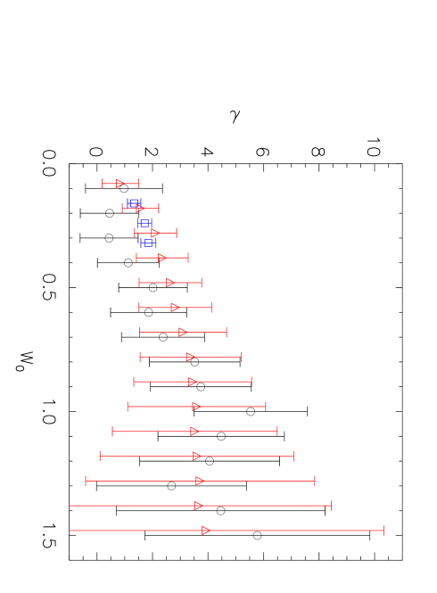
Figure 2: The maximum likelihood estimate of the power law index $\gamma$ vs. rest equivalent width threshold $W_{0}$, with $1\sigma$ error bars. Open circles show the observed data and triangles the mean of 1000 Monte Carlo simulations (offset by $\Delta z=-0.02$ for clarity); squares represent the results of Bechtold (1994) for the first three samples in her Table 4 (absorption $z<z_{QSO}-0.15$, medium and low resolution samples combined).

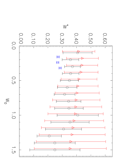
Figure 3: The maximum likelihood rest equivalent width distribution index $W^{*}$ vs. rest equivalent width detection threshold $W_{0}$. Open circles show observed data and triangles the mean of 1000 Monte Carlo simulations (offset by $\Delta W_{0}=-0.02$ Å for clarity). Squares represent the results of Bechtold (1994) for the first three samples in her Table 4 (absorption $z<z_{QSO}-0.15$, medium and low resolution samples combined). Error bars indicate $1\sigma$ uncertainties. The lower values of $W^{*}$ for the Bechtold data likely arise from the higher resolution of her spectra.

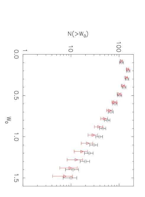
Figure 4: The cumulative number of lines greater than rest equivalent width $N(>W_{0})$ for the data (open circles) and simulations (triangles), with $1\sigma$ uncertainties marked by error bars, for the redshift range $2.15<z<3.26$. The simulations have been offset by $\Delta W_{0}=-0.02$ Å for clarity.

We used between 100 and 1000 synthetic spectra as controls for the calculations in this paper.

3.2 Search for structures extended in three dimensions

We used two different methods to search for correlations of Ly$\alpha$ forest absorbers in three dimensions: (1) the two point correlation function, and (2) the redshift number density.

1. Two point correlation function:  We constructed the two point correlation function in three dimensions as in Paper I. However, we did not use the estimator $DR$ of Davis & Peebles (1983), in which the observed data ($D$) are cross-correlated with a randomly generated data set ($R$) to provide the normalization for the distribution for the absorber pairs. The absorption line density is so high in the higher redshift portion of our data that we would not be able to detect absorber separations much smaller than observed. Rather, we used the $DD/RR$ estimator, and computed the average and first moment about the mean of the two point correlation function directly from the simulations. We found no significant signal in the observed data, nor in any subset of the data as a function of redshift or rest equivalent width detection threshold.

We performed a heuristic check that our algorithm would indeed reveal any clustering, by creating an artificial cluster in the simulated data. The artificial cluster was produced by adding a 100% overdensity of absorbers in the redshift range $2.700<z<2.765$ into the input line list used for a set of simulated spectra; these absorbers are common and identical for all quasars of a given set. Their characteristics ($z,N_{\mathrm{H}I},b)$ were obtained following the same procedure that produces the input line list described above. The redshift range is the best-sampled one in our data, as it is probed, at least partially, by six QSO sightlines for which we have high signal to noise ratio spectra. This artificial cluster would cover approximately $35\times 20h^{-2}$ comoving Mpc² on the plane of the sky, and span $25h^{-1}$ comoving Mpc along the line of sight; it would be as extended along the line-of-sight as the C iv groups described in Paper I, and slightly wider on the plane of the sky.

We produced 100 simulated sets of spectra with such an artificial cluster, and determined the corresponding three dimensional correlation function in the same way as for the observed data. Due to line blending, the mean number of “detected” lines in the artificially overdense region increases only by 27%, compared to the mean number of lines in the simulated spectra with no artificial cluster. However, the mean rest equivalent width of the lines in that interval increases by 41% from $\langle W_{0,{\mathrm{r}andom}}\rangle=0.66$ Å to $\langle W_{0,{\mathrm{c}luster}}\rangle=0.93$ Å, but is not detected significantly since the first moment about the mean is $\sigma(W_{0})\sim 0.6$Å  in both cases.

Similarly, we created artificially clustered data sets with overdensities of 25% and 100% at $2.200<z<2.300$. We do not find any evidence for a significant signal in three dimensional two point correlation function for any of the artificially correlated cases.

2. Redshift number density:  For a second test, we computed the redshift distributions of the observed absorbers toward all lines of sight in our sample. We compare the observed number of absorbers $d{\cal N}_{\rm obs}/dz$ with the expected mean and first moment about the mean from the simulations $d{\cal N}_{\rm exp}/dz$, $\sigma(d{\cal N}_{\rm exp}/dz)$, to define a significance level $\mbox{$SL_{d{\cal N}/dz}$}\equiv(d{\cal N}_{\rm obs}/dz-d{\cal N}_{\rm exp}/dz)/\sigma(d{\cal N}_{\rm exp}/dz)$. The data produce no significant features in $d{\cal N}/dz$ for a variety of rest equivalent width detection thresholds (Figure 5). The most significant feature is an overdensity of lines ($\mbox{$SL_{d{\cal N}/dz}$}\approx 2$) at $2.2<z<2.3$ which is strongest when weak lines ($W_{0}\geq 0.1-0.4$ Å) are included in the sample. This redshift range partially includes the one covered by a group of C iv absorbers found in Paper I, whose corresponding Ly$\alpha$ lines have already been removed from our sample. We therefore find no significant evidence for an overdensity of absorbers in a given redshift interval in the observed data.

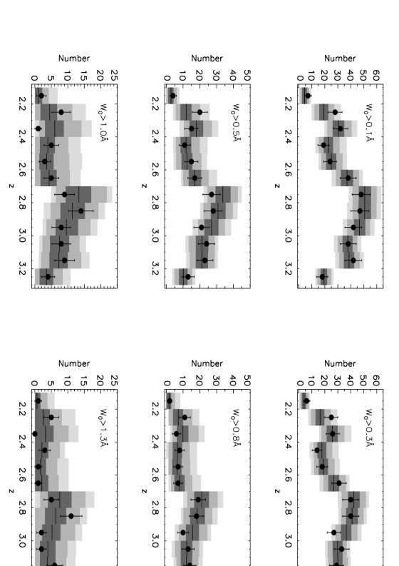
Figure 5: The redshift distribution of the observed data (filled circles, with Poissonian error bars) overlaid against the mean of 1000 Monte Carlo simulations (horizontal lines), for a range of rest equivalent width minimum values. The 68%, 95% and 99% confidence intervals are shown by the dark, medium and light grey shaded regions.

To test the sensitivity of the redshift distribution to the presence of clustered Ly$\alpha$ lines, we also calculated $d{\cal N}/dz$ for the three artificially clustered data sets. Only the 100% overdense case at $2.2<z<2.3$ produces a detectable signal (at $\mbox{$SL_{d{\cal N}/dz}$}\sim 3-4$ level) in the line number density (Figure 6).

Figure 6: The open circles show the significance level $SL_{d{\cal N}/dz}$ of the number of absorption lines in the redshift number density distribution $d{\cal N}/dz$ of absorption lines at $2.70<z<2.80$, for a simulated 100% overdensity of lines at $2.700<z<2.765$, for a series of rest equivalent width detection thresholds $W_{0}$. The first moment about the mean scatter is indicated by the vertical lines. The squares are for a similar 25% overdensity (offset by $W_{0}=0.02$ Å for clarity) and the triangles are for a 100% overdensity at $2.200<z<2.300$ (offset by $W_{0}=-0.02$ Å). We used 100 simulated data sets with no overdensity as controls. At the resolution of our spectra, the largest effect of an overdensity is to increase the measured rest equivalent width of absorption lines, rather than to increase the number of detected lines.

We do not detect any significant structures extended in three dimensions in the observed data, and also conclude that the three dimensional two point correlation function is a less sensitive indicator of clustering in the Ly$\alpha$ forest in three dimensions than the redshift number density.

3.3 Search for structures in the plane of sky

In contrast to the two point correlation function in three dimensions, the two point correlation function in velocity space $\xi(\Delta v)$ has successfully revealed (apparent) clustering (as there is no way to separate out peculiar velocities) in the Ly$\alpha$ forest between lines of sight on the scale of up to 3 arcmin ([15]). In order to extend the exploration of such correlations on scales up to 69 arcmin, we calculated $\xi(\Delta v(\lambda_{\rm i},\lambda_{\rm j}))$, where $\Delta v(\lambda_{\rm i},\lambda_{\rm j})=2~{}c_{s}~{}(\lambda_{\rm i}-\lambda_{\rm j})/(\lambda_{\rm i}+\lambda_{\rm j})$ is the velocity difference between two lines detected at $\lambda_{\rm i}$ and $\lambda_{\rm j}$ in the spectra of two different  quasars, where $c_{s}$ is the speed of light. We computed the first moment about the mean $\sigma(\xi)$ directly from the simulated control sample line lists.

A 50 km s^-1 bin size was chosen, which is more than 3 times larger than the typical error on the determination of the observed lines centroid. It is large enough so that each bin contains on average at least 67 lines drawn from the control sample. This test is sensitive for structures with large transverse extent in the plane of the sky, but not necessarily large extent along the line of sight.

3.3.1 A significant signal at $2.60<z<3.26$?

If we include the entire redshift range of our data sample, the most deviant feature of the two point correlation function $\xi(\Delta v)$ is a $2.7\mbox{$\sigma(\xi)$}$ excess of pairs with $W_{0}\geq 0.1$ Å Ly$\alpha$ absorption lines and velocity differences $50<\Delta v/({\mathrm{k}m\,s}^{-1})<100$ (Figure 7). We then divided the sample using criteria based on the redshift, rest equivalent width and angular separation between the different lines of sight to search for the origin of this possible signal.

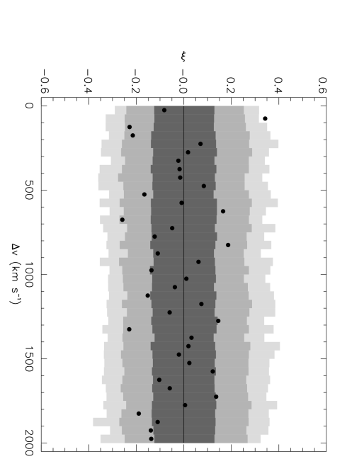
Figure 7: The two point correlation function $\xi(\Delta v)$ for the observed lines, with rest equivalent width threshold $W_{0}\geq 0.1$ Å and covering $2.15<z<3.26$, the entire redshift range over which there are data for at least two lines of sight. Only pairs between different  lines of sight are counted. The dark, medium and light shadings signify the 68%, 95% and 99% confidence limits determined by 1000 Monte Carlo simulations as described in the text.

Limiting the line redshifts to the range $2.60<z<3.26$ reveals an overdensity of line pairs significant at the $3.2\mbox{$\sigma(\xi)$}$ confidence level (Figure 8 and Table 1): our observations provide 79 pairs of $W_{0}\geq 0.1$ Å lines in the $50<\Delta v/({\mathrm{k}m\,s}^{-1})<100$ velocity bin, an excess of 42% compared to a mean and $1\sigma$ dispersion of only $55.6\pm 7.4$ derived from the control sample. The probability of finding such an excess in any bin is $P=0.0012$. Surprisingly, we do not detect any significant signal at velocity splittings $\Delta v<50$ km s^-1, a point which we will examine in detail later (§3.3.5).

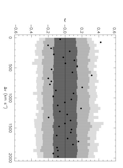
Figure 8: The two point correlation function $\xi(\Delta v)$ for the observed lines, with rest equivalent width threshold $W_{0}\geq 0.1$ Å and confidence limits as in Figure 7, but for $2.60<z<3.26$.

Table 1: Redshift dependence of the feature at $50<\Delta v/\mbox{{\rm km~{}s}${}^{-1}$}\ <100$ for $W_{0}\geq 0.1$ Å.

$z$ range	sample size	$N_{\rm exp}\pm\sigma_{\rm exp}$	$N_{\rm obs}$	SL
2.16–2.40	067	0$7.3\pm 3.7$	09	0.5
2.40–2.60	043	0$3.1\pm 1.7$	03	–0.1
2.60–2.80	086	$18.2\pm 4.2$	26	1.9
2.80–3.00	089	$19.6\pm 4.0$	32	3.1
3.00–3.26	098	$16.7\pm 4.1$	21	1.0
2.60–3.26	273	$55.6\pm 7.4$	79	3.2

The low redshift range $2.16<z<2.60$ does not present any significant signal at any velocity splitting, but the small number of expected line pairs per velocity bin (3.1 to 7.3, see first two rows in Table 1) hinders the detection of all but the very strongest correlation.

3.3.2 Rest equivalent width dependence

In a similar way, we calculated $\xi(\Delta v)$ for subsamples of $2.60<z<3.26$ lines based on their rest equivalent width. Table 2 shows that the significance of the correlation is larger for low values of the minimum rest equivalent width threshold: it is quite strong (3.6$\sigma(\xi)$) for $0.1\leq W_{0}/{\rm\AA}<0.7$, and reaches 4.0$\sigma(\xi)$ for $0.1\leq W_{0}/{\rm\AA}<0.9$. However, the significance of the signal rapidly decreases for increasing minimum values of $W_{0}$. If the real value of $\xi=0.5$, the small number of lines prevents the detection of signal at the $3\sigma$ significance level for $W_{0}\geq 0.4$ Å. Therefore, we can only conclude that the value of the correlation function does not increase strongly with the minimum equivalent width of the lines.

Table 2: Rest equivalent width dependence of the feature at $50<\Delta v/\mbox{{\rm km~{}s}${}^{-1}$}\ <100$ for $2.60<z<3.26$.

$W_{0}$ range (Å)	sample size	$N_{\rm exp}\pm\sigma_{\rm exp}$	$N_{\rm obs}$	SL
$W_{0}\geq 0.1$	273	$55.6\pm 7.4$	79	3.2
$W_{0}\geq 0.2$	251	$47.3\pm 6.8$	70	3.4
$W_{0}\geq 0.3$	217	$35.8\pm 5.9$	47	1.9
$W_{0}\geq 0.4$	185	$26.4\pm 5.3$	32	1.1
$W_{0}\geq 0.5$	155	$18.8\pm 4.5$	22	0.7
$W_{0}\geq 0.6$	127	$12.7\pm 4.0$	11	-0.7-
$0.1\leq W_{0}<0.4$	188	$\phantom{1}5.2\pm 2.6$	8	1.1
$0.1\leq W_{0}<0.5$	118	$\phantom{1}9.6\pm 3.4$	20	3.1
$0.1\leq W_{0}<0.6$	146	$15.1\pm 4.0$	24	2.2
$0.1\leq W_{0}<0.7$	165	$19.6\pm 4.3$	35	3.6
$0.1\leq W_{0}<0.8$	181	$23.8\pm 4.5$	40	3.5
$0.1\leq W_{0}<0.9$	200	$29.1\pm 5.2$	50	4.0
$0.1\leq W_{0}<1.0$	216	$34.1\pm 5.6$	54	3.5

We also investigated whether the pairs of $W_{0}\geq 0.1$ Å absorbers within the $50<\Delta v/{\rm km\,s}^{-1}<100$ bin tend to present similar equivalent widths. We define $\Delta W_{0,i,j}\equiv|W_{0,i}-W_{0,j}|$ for lines $i,j$ of the sample. The distribution of $\Delta W_{0,i,j}$ in that bin is not significantly different from that of the data as a whole. Therefore, the line pairs which produce the signal do not possess a significantly high proportion of pairs of lines with similar rest equivalent widths.

3.3.3 Angular separation dependence

We investigated the dependence of the signal strength on the angular separation $\Delta\theta_{\rm i,j}$ between the background quasars. The seven QSOs which contribute Ly$\alpha$ lines to the sample at $2.60<z<3.26$ have angular separations of $6.1<\Delta\theta/{\rm arcmin}<41.2$. However, QSO 0041–2707 contributes only 9 of the 273 lines in the sample and provides a separation of $\Delta\theta\sim 41$ arcmin only with QSO 0042–2627 and QSO 0043–2633 for 3% of the line pairs; the other 97% of the line pairs come from QSOs with angular separation $6.1<\Delta\theta/{\rm arcmin}<31.2$. We split the sample of line pairs (i.e., lines with $W_{\rm 0}>0.1$ Å and $2.60<z<3.26$) into two parts of similar size: the lines detected in the spectra of quasars separated by $\Delta\theta<24$ and $\Delta\theta>24$ arcmin formed the small and large $\Delta\theta$ samples, respectively. We find an excess of 8 line pairs (33 compared to $24.7\pm 5.0$ expected) with $50<\Delta v/\mbox{{\rm km~{}s}${}^{-1}$}<100$ in the small $\Delta\theta$ sample, a 1.7$\sigma(\xi)$ overdensity. The large $\Delta\theta$ sample produces a 2.8$\sigma(\xi)$ excess of 15 line pairs (46 compared to $30.8\pm 5.4$) in the same velocity bin. Therefore neither half of the sample produces a significant correlation on its own.

However, two lines of sight (towards 0042–2627 and 0042–2656, $\Delta\theta=29.1$ arcmin) provide 27% of the total number of pairs in the $50<\Delta v/\mbox{{\rm km~{}s}${}^{-1}$}<100$ bin, with 21 pairs observed while only $14.3\pm 1.6$ are expected. They also are the QSOs which contribute most to the number of absorption lines in the $z>2.60$ range. The large number of absorption systems toward each QSO, and the overabundance of pairs between them, lead us to suspect that perhaps each of these 2 spectra were contaminated by metal line systems from absorbers which, coincidentally (or not) lie at the same redshift, but for a velocity difference of $50<\Delta v/{\rm\mbox{{\rm km~{}s}${}^{-1}$}}<100$. We have investigated this possibility but were forced to reject it for two reasons. (A) If the signal would actually come from metal lines, they would appear clustered in redshift, either because some of them would be doublets (Mg ii, Al iii, C iv) or have recognizable line separations (e.g. lines from Fe i, Fe ii, etc.). We do not see this effect: on the contrary, the lines contributing to the signal are well-spread over the whole common redshift range. (B) We searched for additional heavy element systems and found candidates for C iv or Mg ii doublets; however, they do not constitute a large number of lines. Higher resolution spectra would be needed to eliminate possibility (B) definitively.

3.3.4 Nearest neighbor distribution

In order to confirm the excess of line pairs with $50<\Delta v/\mbox{{\rm km~{}s}${}^{-1}$}<100$, we also calculated the nearest neighbor distribution $NN(\Delta v)$ and its first moment about the mean $\sigma(NN)$, which provides a more sensitive test for correlations at small separations than the two point correlation function: it reveals a $2.9\mbox{$\sigma(NN)$}$ overdensity of line pairs at $50<\Delta v/{\rm\mbox{{\rm km~{}s}${}^{-1}$}}<100$ (Figure 9). The Kolmogorov-Smirnov (KS) test, which is independent of the velocity binning, indicates the likelihood of the observed data being consistent with the random control sample to be $P=0.0001$. We also computed the variance ${\cal V}$ of the nearest neighbor function $NN(\Delta v)$ for each simulation $j$ over the velocity bins $\Delta v_{i}$,

$${\cal V}_{j}\equiv\sum_{i}(NN(\Delta v_{j,i})-\langle NN(\Delta v_{i})\rangle)^{2}\frac{\langle NN(\Delta v_{i})\rangle}{\sum_{i}\langle NN(\Delta v_{i})\rangle}$$ (7)

where the means are taken over all simulations $j$ (Figure 10). The observed variance is exceeded by that of the simulations in 36 cases out of 1000. The KS test and the distribution of variances indicate that the probability of the observed nearest neighbor distribution arising from a random distribution of absorbers is small, though the exact probability is difficult to determine because the estimates between the two methods differ by a factor of 360. A better understanding of the signal can be obtained with a more detailed model, which we describe in the next section.

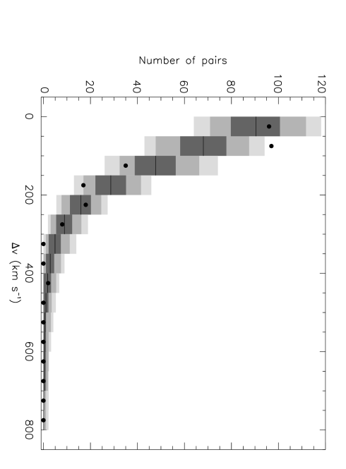
Figure 9: The nearest neighbor distribution for the observed lines ($W_{0}\geq 0.1$ Å) at $2.60<z<3.26$. The dark, medium and light shadings signify the 68%, 95% and 99% confidence limits determined by 1000 Monte Carlo simulations as described in the text. There is a $2.9\sigma$ overdensity of line pairs at $50<\Delta v<100$ km s^-1.

Figure 10: The distribution of variances in the nearest neighbor distribution $NN(\Delta v)$ for 1000 Monte Carlo simulations. The dashed line indicates the variance for the observed lines, which is exceeded by 3.6% of the Monte Carlo simulations.

3.3.5 A model for the signal

The origin of the correlation is mysterious if the result is taken at face value, that is, if the excess of pairs really occurs at $50<\Delta v/\mbox{{\rm km~{}s}${}^{-1}$}<100$, and does not actually peak at $0<\Delta v/\mbox{{\rm km~{}s}${}^{-1}$}<50$. Indeed, all physically plausible models which we have considered, i.e. sheets, filaments or any other connected structures spanning 30 arcmin on the sky, that would give a signal between $50<\Delta v/\mbox{{\rm km~{}s}${}^{-1}$}<100$ at large angular separation, would also give a signal between $0<\Delta v/\mbox{{\rm km~{}s}${}^{-1}$}<50$ at small $\Delta\theta$. Since the number of line pairs per bin is comparable at $\sim 10,20$ and 30 arcmin, any such model would lead to a signal of similar strength in these two velocity bins.

As the accuracy of the line wavelength is thought to be of the order 13 km s^-1, if the ‘real’ correlation is actually at $0<\Delta v/\mbox{{\rm km~{}s}${}^{-1}$}<50$, the effect of underestimating the accuracy of the line center measurement would a priori only broaden the peak of the correlation, not its centroid. However, the blending of several Ly$\alpha$ lines due to the low spectral resolution can account for the observed $\Delta v$ of the correlation peak if the signal to noise ratio is not very good.

In order to test this hypothesis, we modified the generation of the simulated spectra described in §3.1. Specifically, we changed the way the input line list is produced before the creation of the Voigt profiles, in such a way as to introduce a correlation between the different lines of sight, while conserving the mean density of (input) lines per unit redshift.

First, we produced a new input line list following the same parameters as the ones described in §3.1, but extending over the redshift range whose limits are the minimal and maximal redshifts covered by our spectra. Let us call this input line list the full-range line list, ${\cal F}=\bigcup_{i=1,n_{\mathrm{f}}}{F_{i}}$, where $F_{i}=(z_{i},N_{{\mathrm{H}I},i},b_{i})$. Similarly, let us call the input line list for the spectra ${\cal S}_{q}=\bigcup_{i=1,n_{\mathrm{q}}}S_{q,i}$, with $S_{q,i}=(z_{q,i},N_{{\mathrm{H}I},q,i},b_{q,i})$, where $q=1,...,10$ identifies the quasar.

Two additional input parameters are needed: $c$, which describes the percentage of input lines to be common to each new input line list, and $\sigma_{\mathrm{c}}$, which gives the velocity dispersion of the common line lists along the different lines-of-sight.

The new input line list ${\cal N}_{q}$ for the quasar $q$ is created in the following way. It is the union of two sets of lines. The first set of lines is common to each quasar. It originates from the full-range line list ${\cal F}$: each line $F_{i}$ has a probability $c$ to be included in each new line list ${\cal N}_{q}$; the values of $N_{{\mathrm{H}I},i}$ and $b_{i}$ are identical in each ${\cal N}_{q}$, but the redshift $z_{i}$ is modified to include a peculiar velocity, whose value follows a Gaussian distribution with the velocity dispersion $\sigma_{\mathrm{c}}$. The second set of lines is unique to each quasar and comes from the line lists ${\cal S}_{q}$: each line $S_{q,i}$ has a probability $(1-c)$ of being included (as it is) in the line list ${\cal N}_{q}$. The rest of the procedure is then identical to the one described in §3.1.

It is important to note that the percentage of common lines in the input line list is not necessarily reflected in the ‘observed’ line list, as mentioned in §3.2. The blending due both to the intrinsic width of the lines and to the 2 Å  spectral resolution (1) leads relatively weak lines to disappear into the wings of stronger lines, and (2) makes several lines with small wavelength separation appear as one. These effects are revealed in the results of the following test.

We computed the value of the two point correlation function for different values of $c$ and $\sigma_{\mathrm{c}}$ by creating 1000 simulations for each pair $(c,\sigma_{\mathrm{c}})$ considered. Figure 11 presents some of the results, expressed in confidence level in the second bin ($50<\Delta v/({\mathrm{k}m}~{}{\mathrm{s}}^{-1})<100$) vs.  the confidence level in the first bin ($0<\Delta v/({\mathrm{k}m}~{}{\mathrm{s}}^{-1})<50$). In each case, the asterisk symbol indicates the values obtained with the observed data.

Figure 11: The overdensity of line pairs in the second ($50<\Delta v/(\mbox{{\rm km~{}s}${}^{-1}$})<100$) bin vs.  the first ($0<\Delta v/(\mbox{{\rm km~{}s}${}^{-1}$})<50$) for the two point correlation function $\xi(\Delta v)$, expressed in units of the first moment about the mean for an average of 1000 Monte Carlo simulations, $\sigma(\xi)$. A series of models were calculated, with varying percentages of artificially correlated lines $c$ and velocity dispersion $\sigma_{\mathrm{c}}$. The asterisk symbol indicates the value derived from the observations.

The top left panel shows the results when no line is (arbitrarily) common between the different lines-of-sight: as expected, there are very few cases where a false positive signal is detected. In this set of 1000 simulations, there is only 1 case when a value is larger than $3\mbox{$\sigma(\xi)$}$ in either of the two bins. We also note two other false positive cases of negative correlation, also at greater than the 3$\sigma(\xi)$ level.

If 10% of the lines are common $(c=0.10)$ to each line-of-sight with a velocity dispersion of $\sigma_{\mathrm{c}}=50~{}{\mathrm{k}m}~{}{\mathrm{s}}^{-1}$ (top middle panel), then the correlation is detected at the $3\mbox{$\sigma(\xi)$}$ level in at least 1 of the two first bins in only about 4% of the cases, with the detection in the 2nd bin alone accounting for 25% of these cases. Even if 20% of the lines are common with $\sigma_{\mathrm{c}}=50~{}{\mathrm{k}m}~{}{\mathrm{s}}^{-1}$, the correlation function does not consistently show any significant signal: moreover, the quadratic sum of the significance level in the two first bins does not reveal any signal at more than 3$\sigma(\xi)$ in 64% of the cases.

Table 3: Percentage of cases that the significance level of the signal is larger than $3.2\sigma$ in at least one of the first 3 bins.

$c$   :	0%	10%	30%	40%	50%	60%	70%	70%	80%
$\sigma_{\mathrm{c}}({\mathrm{k}m}~{}{\mathrm{s}}^{-1})$   :		50	100	150	200	200	200	250	250
	0.2	2.5	7.4	7.0	8.7	17.2	33.8	22.2	40.2

As can be seen in the different panels, the effect of increasing the number of common lines $c$ is to move the set of points approximately along the diagonal of equal confidence limits towards larger values, while a larger velocity dispersion increases their spread perpendicular to this direction and reduces the number of bins with significant signals. These simulations, whose results are summarized in Table 3, show that it is unlikely that the signal that we detect is a statistical fluke; on the contrary, it probably indicates that a significant number of lines are common between the different lines-of-sight with a velocity dispersion probably larger than $100~{}{\mathrm{k}m}~{}{\mathrm{s}}^{-1}$. Unfortunately, the limited spectral resolution of our data does not allow us to quantify this result better.

4 Discussion

We have searched for correlations among a sample of 383 $W_{0}\geq 0.1$ Å (5$\sigma$ detection threshold) Ly$\alpha$ absorbers ranging over $2.15<z<3.26$ in front of 10 QSOs separated by $6.1<\Delta\theta/{\rm arcmin}<69$, an angular separation an order of magnitude greater than for any other study for more than a simple pair of QSOs. Our statistical tests have consisted of the three dimensional two point correlation function, the redshift distribution $d{\cal N}/dz$, and the two point correlation function in redshift space. We have found no evidence for clustering in the the three dimensional two point correlation function, and no anomalies in the absorber redshift distribution $d{\cal N}/dz$. In fact, we find that the three dimensional two point correlation function is less sensitive to clusters of Ly$\alpha$ absorbers than $d{\cal N}/dz$.

We have calculated the two point correlation function in velocity space and find a signal of $\xi(\Delta v)=0.35$ with significance $3.2\mbox{$\sigma(\xi)$}$ at velocity separation $50<\Delta v/({\rm\mbox{{\rm km~{}s}${}^{-1}$}})<100$ for a subsample at $2.60<z<3.26$ and $W_{0}\geq 0.1$ Å. Its significance rises to $4.0\mbox{$\sigma(\xi)$}$ if the rest equivalent width is restricted to $0.1<W_{0}/{\rm\AA}<0.9$, but tends to weaken with increasing minimum values of $W_{0}$. However, given the limited sample size, we do not draw any stronger conclusion than that the significance of the signal does not strongly increase with the minimum value of $W_{0}$.

Additional simulations show that blending due to the low spectral resolution of our spectra may often destroy any signal even if most of the lines are common between the lines of sight. However, they also show that if any signal is detected in any of the first few bins, it is unlikely to be due to chance. Instead, such a signal very often reveals the presence of an underlying correlation. If the correlation that we find is only the strongest part of an underlying distribution, which may extend over a larger range in velocity space, then the analysis of a larger and higher resolution data sample should confirm the reality of the feature.

Physically, a correlation at such a small velocity dispersion could arise from the apparent collapse of structures along the line of sight (the “bull’s-eye effect”, [56]; [41]), reducing their apparent extent in velocity space. Furthermore, if such structures contain Ly$\alpha$ absorbers on the scale of 10–30 arcmin, or 8.7–26 (13–40) $h^{-1}$ comoving Mpc for $\Omega=1.0$ (0.2), then density gradients within the structures could explain the difference between the clustering of strong absorbers that Crotts & Fang found on small angular scales, and of weaker absorbers which we find on larger scales. Overdensities and underdensities on the scale of a few tens of comoving Mpc have been identified along individual lines of sight ([12]), so similar features in the plane of the sky are plausible.

Oort (1981, 1983, 1984) suggested that correlated Ly$\alpha$ absorption on $0.5-1^{\circ}$ scales could be the signature of high redshift superclusters arising from “pancake” formations. Simulations of the growth of cosmological structures ([52]; [28]; [46]; [57]; [67], 1998) indicate that structures (e.g. filaments/sheets) of dark matter and gas extend up to several Mpc, forming a “cosmic web” ([4]). Such structures produce Ly$\alpha$ absorption up to 7 comoving Mpc from luminous galaxies or groups of galaxies ([52]). The detailed analysis of simulations can yield quantitative predictions for the Ly$\alpha$ forest correlation function in the larger context of galaxy formation (on scales of $\sim 1h^{-1}$ Mpc, [7]), and permit the recovery of power spectrum of density perturbations (on scales of up to $11h^{-1}$ Mpc, [13]), though at present, the small size of the simulation boxes does not permit similar predictions on the scale probed by our data. Our observations indicate that structures coherent over more than 7 comoving Mpc may well exist in the Ly$\alpha$ forest at $z\sim 3$. As simulations become more advanced and box sizes increase, it will be possible to compare model structures to those of the scale we find in our data.

The correlations of the Ly$\alpha$ lines in velocity space imply large scale structure extending over 30 arcmin , or about $26\,(40)h^{-1}$ comoving Mpc for $\Omega=1.0\,(0.2)$. The comparison between Ly$\alpha$ absorbers on such wide angular scales provides a unique tool to probe the evolution of large scale structure at high redshift. With 8–10m class telescopes, it will be possible to survey fainter QSOs, which would provide a much higher density per unit area on the sky and thus enable a much more detailed probe of the correlation behavior of QSO absorption systems. It will also be possible to detect routinely bright galaxies in the vicinity of such correlated absorbers, to reveal more details about the relationship between the two sorts of objects and to the distribution of matter in general.

References

- Bechtold [1994] Bechtold, J. 1994, ApJS, 91, 1
- Bechtold et al. [1994] Bechtold, J., Crotts, A. P. S., Duncan, R. C., & Fang, Y. 1994, ApJ, 437, L83
- Bi & Davidsen [1997] Bi, H., & Davidsen, A. F. 1997, ApJ, 479, 523
- Bond et al. [1996] Bond, J. R., Kofman, L., & Pogosyan, D. 1996, Nature, 380, 603
- Bowen, Pettini, & Blades [1996] Bowen, D. V., Blades, J. C., & Pettini, M. 1996, ApJ, 464, 141
- Cen et al. [1994] Cen, R., Miralda-Escudé, J., Ostriker, J. K., & Rauch, M. 1994, ApJ, 437, L9
- Cen & Simcoe [1997] Cen, R., & Simcoe, R. A. 1997, ApJ, 483, 8
- Charlton et al. [1997] Charlton, J. C., Anninos, P., Zhang, Y., & Norman, M. L. 1997, ApJ, 485, 26
- Chen et al. [1998] Chen, H.-W., Lanzetta, K. M., Webb, J. K., & Barcons, X. 1998, ApJ, 498, 77
- Cowie et al. [1995] Cowie, L. L., Songaila, A., Kim, T.-S., & Hu, E. M. 1995, AJ, 109, 1522
- Cristiani et al. [1995] Cristiani, S., d’Odorico, S., Fontana, A., Giallongo, E., & Savaglio, S. 1995, MNRAS, 273, 1016
- Cristiani et al. [1997] Cristiani, S., d’Odorico, S., d’Odorico, V., Fontana, A., Giallongo, E., & Savaglio, S. 1997, MNRAS, 285, 209
- Croft et al. [1998] Croft, R. A. C., Weinberg, D. H., Katz, N., & Hernquist, L. 1997, ApJ, 495, 44
- Crotts [1989] Crotts, A. P. S. 1989, ApJ, 336, 550
- Crotts & Fang [1998] Crotts, A. P. S., & Fang, Y. 1998, ApJ, 502, 16
- Davé et al. [1999] Davé, R., Hernquist, L., Katz, N., & Weinberg, D. 1999, ApJ, 511, 521
- Davis & Peebles [1983] Davis, M., & Peebles, P. J. E. 1983, ApJ, 267, 465
- Dinshaw et al. [1994] Dinshaw, N., Impey, C. D., Foltz, C. B., Weymann, R. J., & Chaffee, F. H. 1994, ApJ, 437, L87
- Dinshaw et al. [1995] Dinshaw, N., Foltz, C. B., Impey, C. D., Weymann, R. J., & Morris, S. L. 1995, Nature, 373, 223
- Dinshaw & Impey [1996] Dinshaw, N., & Impey, C. D. 1996, ApJ, 458, 73
- Dinshaw et al. [1997] Dinshaw, N., Weymann, R. J., Impey, C. D., Foltz, C. B., Morris, S. L., & Ake, T. 1997, ApJ, 491, 45
- Dobrzycki [99] Dobrzycki, A. 1999, private communication
- D’Odorico et al. [1998] D’Odorico, V., Cristiani, S., Fontana, A., Giallongo, E., & Shaver, P. 1998, A&A, 339, 678
- Fang et al. [1996] Fang, Y., Duncan, R. C., Crotts, A. P. S., & Bechtold, J. 1996, ApJ, 462, 77
- Fernández-Soto et al. [1996] Fernández-Soto, A., Lanzetta, K. M., Barcons, X., Carswell, R. F., Webb, J. K., & Yahil, A. 1996, ApJ, 460, L85
- Foltz et al. [1984] Foltz, C. B., Weymann, R. J., Röser, H.-J., & Chaffee, F. H. 1984, ApJ, 281, L1
- Grogin & Geller [1998] Grogin, N.A., & Geller, M.J., 1998, ApJ, 505, 506
- Hernquist et al. [1996] Hernquist, L., Katz, N., Weinberg, D. H., & Miralda-Escudé, J. 1996, ApJ, 457, L51
- Hu et al. [1995] Hu, E., Kim, T-S., Cowie, L. L., Songaila, A., & Rauch, M. 1995, AJ, 110, 1526
- Impey, Petry, & Flint [1999] Impey, C.D., Petry, C.E., & Flint, K.P., 1999, ApJ, in press, astro-ph/9905381
- Khare et al. [1997] Khare, P., Srianand, R., York, D. G., Green, R., Welty, D., Huang, K-L., & Bechtold, J. 1997, MNRAS, 285, 167
- Kim et al. [1997] Kim, T.-S., Hu, E. M., Cowie, L. L., & Songaila, A., 1997, AJ, 114, 1
- Kirkman & Tytler [1997] Kirkman, D., & Tytler, D., 1997, ApJ, 484, 672
- Lanzetta et al. [1995] Lanzetta, K. M., Bowen, D. V., Tytler, D., & Webb, J. K. 1995, ApJ, 442, 538
- Le Brun, Bergeron, & Boissé [1996] Le Brun, V., Bergeron, J., & Boissé, P. 1996, A&A, 306, 691
- Liske et al. [1999] Liske, J., Webb, J. K., Williger, G. M., Fernández-Soto, A., & Carswell, R. F. 1999, MNRAS, in press, astro-ph/9910407
- Lu, Wolfe, & Turnshek [1991] Lu, L., Wolfe, A. M., & Turnshek, D. A., 1991, ApJ, 367, 19
- Lynds [1971] Lynds, R. 1971, ApJ, 164, L73
- McDonald & Miralda-Escudé [1999] McDonald, P., & Miralda-Escudé, J. 1999, ApJ, 518, 24
- Meiksin & Bouchet [1995] Meiksin, A., & Bouchet, F. 1995 ApJ, 448, L85
- Melott et al. [1998] Melott, A. L., Coles, P., Feldman, H. A., & Wilhite, B. 1998, ApJ, 496, L85
- Miralda-Escudé & Rees [1997] Miralda-Escudé, J., & Rees, M. J. 1997, ApJ, 478, L57
- Mo & Morris [1994] Mo, H.M., & Morris, S. L. 1994, MNRAS, 269, 52
- Morris et al. [1993] Morris, S. L., Weymann, R. J., Dressler, A., McCarthy, P. J., Smith, B. A., Terrile, R. J., Giovanelli, R., & Irwin, M. 1993, ApJ, 419, 524
- Morris & van den Berg [1994] Morris, S. L., & van den Bergh, S. 1994, ApJ, 427, 696
- Mücket et al. [1996] Mücket, J., Petitjean, P., Kates, R. E., & Riediger, R. 1996, A&A 308, 17
- Oort [1981] Oort, J. H. 1981, A&A, 94, 359
- Oort [1983] Oort, J. H. 1983, ARA&A, 21, 373
- Oort [1984] Oort, J. H. 1984, A&A, 139, 211
- Ostriker, Bajtlik, & Duncan [1988] Ostriker, J. P., Bajtlik, S., & Duncan, R. C. 1988, ApJ, 327, L35
- Parnell & Carswell [1988] Parnell, H.C., & Carswell, R.F. 1988, MNRAS, 230, 491
- Petitjean, Mücket & Kates [1995] Petitjean, P., Mücket, J. P., & Kates, R. E. 1995, A&A, 295, L9
- Petitjean et al. [1993] Petitjean, P., Webb, J.K., Rauch, M., Carswell, R.F., & Lanzetta, K. 1993, MNRAS, 262, 499
- Petitjean et al. [1998] Petitjean, P., Surdej, J., Smette, A., Shaver, P., Mücket, J., & Remy, M. 1998, A&A, 334, L45
- Pierre et al. [1990] Pierre, M., Shaver, P. A., & Robertson, J. G. 1990, A&A, 235, 15
- Praton, Melott, & McKee [1997] Praton, E. A., Melott, A. L., & McKee, M. Q. 1997, ApJ, 479, 15
- Rauch, Haehnelt, & Steinmetz [1997] Rauch, M., Haehnelt, M. G., & Steinmetz, M. 1997, ApJ, 481, 601
- Sargent et al. [1980] Sargent, W. L. W., Young, P. J., Boksenberg, A., & Tytler, D. 1980, ApJS, 42, 41
- Shull et al. [1998] Shull, J. M., Penton, S. V., Stocke, J. T., Giroux, M. L., van Gorkom, J. H., Lee, Y. H., & Carilli, C. 1998, AJ, 116, 2094
- Smette et al. [1992] Smette, A., Surdej, J., Shaver, P. A., Foltz, C.B., Chaffee, F. H., Weymann, R. J., Williams, R. E., & Magain, P. 1992, ApJ, 389, 39
- Smette et al. [1995] Smette, A., Robertson, J. G., Shaver, P. A., Reimers, D., Wisotzki, L., & Köhler, Th. 1995, A&AS, 113, 199
- Songaila & Cowie [1996] Songaila, A., & Cowie, L. L. 1996, AJ, 112, 335
- Tripp, Lu, & Savage [1998] Tripp, T. M., Lu, L., Savage, B. D., 1998, ApJ, 508, 200
- van Gorkom et al. [1996] van Gorkom, J. H., Carilli, C. L., Stocke, J. T., Perlman, E. S., & Shull, J. M. 1996, AJ, 112, 1397
- Williger et al. [1996] Williger, G. M., Hazard, C., Baldwin, J. A., & McMahon, R. G. 1996, ApJS, 104, 145 (Paper I)
- Webb [1987] Webb, J. K. 1987, in Observational Cosmology, Proc. IAU Symp. 124, eds. Hewett, A., Burbidge, G., Fang, L. Z. (Dordrecht: Kluwer), 803
- Zhang et al. [1997] Zhang, Y., Anninos, P., Norman, M. L., & Meiksin, A. 1997, ApJ, 485, 496
- Zhang et al. [1998] Zhang, Y., Meiksin, A., Anninos, P., & Norman, M. L. 1998, ApJ, 495, 63