Radiation from cosmic string standing waves

Abstract

We have simulated large-amplitude standing waves on an Abelian-Higgs cosmic string in classical lattice field theory. The radiation rate falls exponentially with wavelength, as one would expect from the field profile around a gauge string. Our results agree with those of Shellard and Moore, but not those of Vincent, Antunes, and Hindmarsh. The radiation rate falls too rapidly to sustain a scaling solution via direct radiation of particles from string length. There is thus reason to doubt claims of strong constraints on cosmic string theories from cosmic ray observations.

Introduction

Cosmic strings are one-dimensional topological defects which may have been created by a phase transition in the early universe [1]. (For reviews see [2, 3].) As the universe evolves, intercommutations between long strings produce oscillating loops. In the standard scenario, these loops lose energy by gravitational radiation and eventually disappear. This produces a scaling solution where the average distance between strings is a constant fraction of the Hubble length. Most of the energy in the string network is emitted as gravitational waves, which we cannot observe, and only a small fraction appears as high-energy particles.

However, in a recent paper [4], Vincent, Antunes, and Hindmarsh claim that energy in a string network is lost by direct particle emission from long strings, rather than in gravitational waves. To back up this claim they study large-amplitude sinusoidal standing waves, and claim that the energy emission rate is sufficient to explain scaling behavior with the great majority of the energy emitted as particles. Moore and Shellard [5] found that the emission rate fell exponentially with wavelength, but their amplitudes [6] were much less than those of [4]. Furthermore, the range of wavelengths in which [5] saw exponential fall off had no overlap with the wavelengths studied in [4].

Here we simulate the same large-amplitude waves as in [4] and cover part of the same wavelength range, but we come to a different conclusion. In our simulations, the energy emission rate declines exponentially with wavelength, and thus cannot account for the large direct-emission rate claimed in [4].

Model

We work with the Abelian-Higgs model, which produces local strings with no massless degrees of freedom in the vacuum. The Lagrangian is

$${\cal L}=D_{\mu}\bar{\phi}D^{\mu}\phi-{1\over 4}F_{\mu\nu}F^{\mu\nu}-{\lambda\over 4}(|\phi|^{2}-\eta^{2})^{2}\,.$$ (1)

We work with units such that $\eta=1$ and $e=1$, and we use the “critical coupling” regime in which $\beta=\lambda/(2e^{2})=1$ so that in our units $\lambda=2$. As in [4], we study strings whose initial core position is given by a sinusoidal wave $y=A\cos kx$, with amplitude $A=\lambda/2=\pi/k$ [7].

A preliminary investigation shows that emission from a standing wave is not uniform in time, but rather consists of a series of bursts emitted when the string is momentarily stationary with large amplitude waves in its position. Figure 1

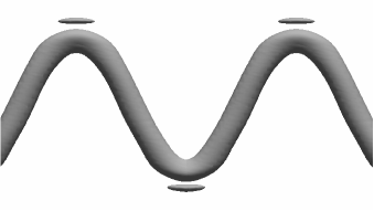
FIG. 1.: A surface of constant energy density shows a sinusoidal wave on a cosmic string and the energy emitted from the high curvature regions.

shows a snapshot of the energy density around a string at one such point, and Fig. 2

FIG. 2.: Energy emitted from one wavelength of a standing wave. The radiation appears as a series of bursts.

shows a plot of the energy emitted over several oscillations.

It thus appears that standing wave radiation is akin to radiation from cusps, and results from the overlap of the tails of the the string fields. We use such a model below to compute a theoretical expectation of the dependence of radiation rate on wavelength.

Expectations

Vincent, Antunes, and Hindmarsh [4] argued as follows: in a scaling network, the distance between strings, $\xi$, scales with the Hubble distance, which is proportional to time. In a volume $\xi^{3}$ there will be string length roughly $\xi$, so the energy density in the string network is $\rho=\mu/\xi^{2}$, and thus $\dot{\rho}=-2\mu\dot{\xi}/\xi^{3}$. Since $\dot{\xi}$ is a constant, $\dot{\rho}\xi^{3}$ is constant. As a model they used a sinusoidal standing wave with wavelength $\lambda$ in a box of volume $\lambda^{3}$. They expected $\dot{\rho}\lambda^{3}$ to be constant. If we let $E$ be the energy of a single wavelength of the string, then $E=\rho\lambda^{3}$, and thus $\dot{E}$ is independent of $\lambda$. If we let $P_{L}$ be the power per unit length radiated from the standing wave, we need

$$P_{L}\propto\lambda^{-1}$$ (2)

to sustain a scaling network from energy emission of this type.

In contrast, analyzing the fields around the string would lead to a different conclusion. A straight, static string is topologically stabilized in a minimum-energy configuration, and so cannot radiate. If the string is curved, then there is the possibility for radiation, but since the fields fall off exponentially toward the vacuum at large distances from the string, one would expect the amount of radiation to be suppressed by an exponential factor depending on the radius of curvature, $R$. This seems in keeping with Fig. 1, which shows the radiation coming from the points of maximum curvature.

As a specific model, one can imagine that an element of momentarily stationary curved string gives up an amount of energy proportional to $\exp(-\alpha R)dl$, where $\alpha$ is a constant of $O(1)$ and $dl$ is the length of the element of string. The total energy emission is then

$$E\propto\int e^{-\alpha R}dl\,.$$ (3)

For a sinusoidal wave, $y=A\cos kx$, the radius of curvature is

$$R={(1+A^{2}k^{2}\sin^{2}kx)^{3/2}\over Ak^{2}\cos kx}\,.$$ (4)

We will consider the region around one of the peaks of the sinusoid. The energy emission is dominated by the region where $x$ is near zero, so that $R$ is small. In this regime, we can approximate

$$R\approx{(1+A^{2}k^{4}x^{2})^{3/2}\over Ak^{2}(1-k^{2}x^{2}/2)}\approx{1\over Ak^{2}}+\left({3\over 2}Ak^{2}+{1\over 2A}\right)x^{2}\,.$$ (5)

In our case, we are going to consider a fixed ratio of amplitude to wavelength, $A=\lambda/2=\pi/k$ so we get

$$R\approx{\lambda\over 2\pi^{2}}+{3\pi^{2}+1\over\lambda}x^{2}\,.$$ (6)

We can now do the integral of Eq. (3), approximating $dl=\sqrt{1+\pi\sin^{2}kx}\,dx$ by just $dx$, and extending the limits of integration to infinity, to get

$$E\propto\sqrt{\lambda}\,e^{-\alpha\lambda/(2\pi^{2})}\,.$$ (7)

Since we keep the amplitude a fixed multiple of the wavelength, the period of the standing wave is just proportional to $\lambda$. If we consider a half wavelength of string, it emits bursts of energy $E$ twice per cycle, so the power is $\propto\lambda^{-1/2}e^{-\beta\lambda}$, and the power per unit length is

$$P_{L}\propto\lambda^{-3/2}e^{-\beta\lambda}\,.$$ (8)

Simulation

The simulation is based on a lattice action, as described in [8]. However, in the present case we have used a different lattice spacings in the 3 cardinal directions. The maximum speed of the string is quite large, and leads to a Lorentz contraction of the field profile in the direction of motion. To accurately represent the fields, the lattice spacing should be proportional to $1/\gamma_{i}=\sqrt{1-v_{i}^{2}}$, where $v_{i}$ is the component of the string velocity along axis $i$. In the $z$ direction, where there is no motion, we have used a lattice spacing of 0.33, which seems to be the largest that gives reliable results. The corresponding spacings in the $x$ and $y$ directions are 0.31 and 0.10 respectively. The Courant condition requires $\Delta t<{({\Delta x}^{-2}+{\Delta y}^{-2}+{\Delta z}^{-2})}^{-1/2}\approx 0.09$, and in our simulations we use $\Delta t=0.08$.

To extract the energy which is emitted by the string, we have used absorbing boundary conditions on the $y$ and $z$ faces and accumulated at each step the amount of energy that they absorb. The conditions are

$$n_{i}D_{i}\phi = -D_{t}\phi\,,$$ (10)

$${\bf E}_{T} = -{\bf n}\times{\bf B}\,,$$ (11)

where $D$ denotes the covariant derivative, ${\bf n}$ the outward normal unit vector on each boundary, and ${\bf E}_{T}\equiv{\bf E}-{\bf n}({\bf E}\cdot{\bf n})$ the transverse component of the electric field. This corresponds to the zeroth-order absorbing boundary condition for free electromagnetism[9]. The energy flowing into the boundary is

$$E_{absorbed}=\int_{\Omega}{\bf S}\cdot d{\bf n}$$ (12)

where $\Omega$ is the boundary surface, and ${\bf S}$ is the Poynting vector, given by

$$S_{j}=-D_{t}\bar{\phi}D_{j}\phi-D_{t}\phi D_{j}\bar{\phi}+({\bf E}\times{\bf B})_{j}\,.$$ (13)

Using Eqs. (Simulation), we can rewrite Eq. (12) as

$$E_{absorbed}=\int_{\Omega}(2|D_{t}\phi|^{2}+|{\bf E}_{T}|^{2})d\Omega\,,$$ (14)

which is easily computed.

To produce the sinusoidal waves, we use the same technique that we used to generate cusps in [8], i.e., we create two traveling wiggles on a straight string that will combine to produce the desired sinusoidal form. (In the Nambu-Goto approximation, the resulting sinusoid would be exact; in our case there will be a distortion of the shape due to the dynamics that occur before it is formed, but this effect will be small because the wiggles out of which the sinusoid forms are not themselves strongly curved.) The initial field configuration for a moving wiggle is known exactly, from a result of Vachaspati [10]. The advantage of this technique is that it does not require the use of relaxation, as is necessary in other field theory simulation schemes [4, 5].

The two original wiggles will overlap to form a single wavelength of the standing wave, from one minimum of $y$ to the next. At this point it is possible to change to periodic boundary conditions in the $x$ direction, so that the straight part of the string is removed, and we are left with a single wavelength of standing wave in a periodic box. This technique was used to produce Figs. 1 and 2, but it is not an accurate method for extracting the radiation rate, because energy coming from different burst is not clearly separated by the time it reaches the boundaries. When each burst of radiation is emitted, the string changes its shape and amplitude and its subsequent evolution does not correspond to a constant amplitude sinusoid any more. Of course, for large enough $\lambda$ this would not matter, but for the wavelengths in the range of our simulation, it makes a significant difference.

To avoid this problem, we allow the original wiggles to pass by each other beyond the point of the overlap, so that they generate just a single burst, and then separate. The place from which the burst is emitted is at the center of the overlapping region, and the string near that point has been following the same evolution as in a real standing wave for a half period, so we feel that this burst accurately represents a single burst of a standing wave oscillation.

Using the expressions given above for the Poynting vector on the boundaries, we can compute the energy absorbed at each time step in our simulation. The energy absorption on the box faces is shown in Fig. 3.

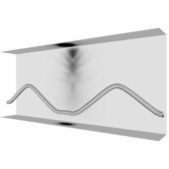
FIG. 3.: Absorption of a burst of energy. The two wiggles have passed through each other and are now separating. Three sides of the bounding box are shown, with darker shades showing areas of greater energy absorption.

Integrating all the energy absorbed from the first burst of radiation we can compute the power emitted by a sinusoidal standing wave.

We have repeated this procedure for different values of the wavelength ranging from $\lambda=12$ to 30, in natural units. In Fig. 4

FIG. 4.: Power per unit length from simulation (points) compared with exponentially decaying model (solid line) and linearly decaying model of [4] (dotted line).

we plot the power emitted per unit length and compare it with theoretical predictions from Eqs. (8) and (2). We see that the exponentially decaying model fits quite well. The line shown has the form

$$P_{L}\propto\lambda^{-3/2}e^{-2.56R_{0}}$$ (15)

with $R_{0}\equiv\lambda/(2\pi^{2})$, but we do not have sufficient accuracy to confirm the exponent of $\lambda$ or the exact constant. A curve with $\lambda^{-2}$ or $\lambda^{-1}$ and somewhat different constant would fit equally well. On the other hand, the form of [4] does not fit at all.

Discussion

We have simulated large-amplitudestanding waves on local cosmic strings, and found an exponential decrease in radiation power with increasing wavelength. Our technique proceeds from separated wiggles with exact initial conditions, and we have used quite a small lattice spacing as compared to other authors, so we feel that our results are reliable.

The constant in the exponential gets its dimensions from the string thickness ($10^{-30}\text{cm}$ for a GUT scale string), and thus for waves of any reasonable cosmological size, the radiation is utterly negligible. One could in principle imagine that strings in cosmological networks still have excitations at wavelengths comparable to their thickness, but this does not seem reasonable. Such wiggles will be rapidly smoothed out by gravitational radiation, and there is no mechanism for regenerating them at such small scales. Thus we conclude that direct radiation of particles from string length cannot play a significant role in the production of cosmic rays or the maintenance of a scaling network. As a result, cosmic ray observations do not rule out field theories that admit cosmic strings, as claimed in [4, 11, 12].

REFERENCES

- [1] T. W. B. Kibble, J. Phys. A9, 1387 (1976).
- [2] A. Vilenkin and E. P. S. Shellard, Cosmic Strings and other Topological Defects. (Cambridge University Press, Cambridge, 1994).
- [3] M. B. Hindmarsh and T. W. B. Kibble, Rep. Prog. Phys. 58, 477 (1995).
- [4] G. Vincent, N. D. Antunes, and M. Hindmarsh, Phys. Rev. Lett. 80, 2277 (1998).
- [5] J. N. Moore and E. P. S. Shellard, hep-ph/9808336 (unpublished).
- [6] Moore and Shellard [5] claim that the ratio of amplitude to wavelength must not exceed in order to avoid the appearance of degenerate “lumps”. However, the present simulations with ratio do not encounter any such problem. It may be that [5] used a form in which the argument of sine is invariant string length, as was used in [13], instead of spatial position as used here.
- [7] Note that unlike the situation with a linear system such as a one-dimensional scalar field, there is nothing special about a sinusoid. In particular, the oscillation period of a sinusoidal standing wave on a string depends on the length along the string, rather than , which is the spatial distance occupied by one wavelength.
- [8] K. D. Olum and J. J. Blanco-Pillado, Phys. Rev. D60, 023503 (1999).
- [9] D. Sheen, SIAM J. Appl. Math. 57, 1716 (1997).
- [10] Vachaspati and T. Vachaspati, Phys. Lett. B 238, 41 (1990).
- [11] U. F. Wichoski, J. H. MacGibbon, and R. H. Brandenberger, hep-ph/9805419 (unpublished).
- [12] P. Bhattacharjee, Q. Shafi, and F. W. Stecker, Phys. Rev. Lett. 80, 3698 (1998).
- [13] R. A. Battye and E. P. S. Shellard, Nucl. Phys. B423, 260 (1994).