Peculiar Velocities and the Mean Density Parameter

Abstract

We study the peculiar velocity field inferred from the Mark III spirals using a new method of analysis. We estimate optimal values of Tully-Fisher scatter and zero-point offset, and we derive the 3-dimensional rms peculiar velocity ($\sigma_{v}$) of the galaxies in the samples analysed. We check our statistical analysis using mock catalogs derived from numerical simulations of CDM models considering measurement uncertainties and sampling variations. Our best determination for the observations is $\sigma_{v}=(660\pm 50)km/s$. We use the linear theory relation between $\sigma_{v}$ , the density parameter $\Omega$, and the galaxy correlation function $\xi(r)$ to infer the quantity $\beta=\Omega^{0.6}/b=0.60^{+0.13}_{-0.11}$ where $b$ is the linear bias parameter of optical galaxies and the uncertainties correspond to bootstrap resampling and an estimated cosmic variance added in quadrature. Our findings are consistent with the results of cluster abundances and redshift space distortion of the two-point correlation function. These statistical measurements suggest a low value of the density parameter $\Omega\sim 0.4$ if optical galaxies are not strongly biased tracers of mass.

Key words: galaxies — distance scale — velocity field — cosmology: density parameter

1 INTRODUCTION

Recent developements on extragalactic distance indicators (Djorgovski and Davis, 1987; Dressler et al., 1987a) allow us to study the peculiar galaxy velocity field in the local Universe up to $\sim 50-100h^{-1}$Mpc (see Giovanelli, 1997, or Strauss and Willick, 1995 for a review). These measurements of peculiar velocities provide direct probes of the mass distribution in the Universe and set constraints on models of large-scale structure formation. By comparing the mass distribution implied by the velocity field with the observed distribution of galaxies the density parameter $\Omega$ can be estimated. Nevertheless, $\Omega$ may only be determined within the uncertainty of the bias parameter $b$ ($b=1/\sigma_{8}$ is the inverse of the root mean square mass fluctuations in spheres of radius$=8Mpc$ $h^{-1}$) through the factor $\beta=\Omega^{0.6}/b$.

Bertschinger & Dekel (1989) developed the POTENT method whereby the mass distribution may be reconstructed by using the analog of the Bernoulli equation for irrotational flows. This method was used to analyse the peculiar velocity field out to 60$h^{-1}$Mpc (Bertschinger et al., 1989). Dekel et al. (1993) compared the previously determined velocity field with the observed distribution of galaxies concluding that $\Omega^{0.6}/b\simeq 1$ provides the best-fitting to the data. Analysis of the velocity tensor (Gorski, 1988; Groth, Juszkiewics and Ostriker, 1989) also provide useful insights on the velocity field. Zaroubi et al. (1997) reconstructed the large-scale power spectrum from the velocity tensor of the MarkIII data and found it consistent with a CDM model with $\sigma_{8}\Omega^{0.6}\simeq 0.8$ although a different result, $\sigma_{8}\Omega^{0.6}\simeq 0.35$, is found by Kashlinsky (1997) in a similar analysis.

Relations between root mean square mass fluctuation in a given scale and density parameter may also be obtained in studies of cluster abundances in different cosmological models. These analysis place constraints of the form $\Omega^{\alpha}/b\simeq 0.4-0.6$ with $\alpha\simeq 0.4-0.6$ in a variety of cold and mixed dark matter models (see Eke et al., 1998, and Gross et al., 1998). Similarly, studies of redshift space distortions of the galaxy two point correlation function also provide a useful restriction to the parameter $\beta$, as for instance Ratcliffe et al. (1997) who find $\beta\simeq 0.5$.

In this paper we study the peculiar velocity field through a statistical analysis of observational data taken from the Mark III catalog. Data characteristics are presented in section 2. Section 3 provides an outline of the statistical procedure. In section 4 we analyse the Mark III spirals, and in section 5 we test our procedure using mock catalogs according to different observers in fully non-linear numerical simulations. In section 6 we provide a determination of the parameter $\beta$.

2 DATA

We use samples of spiral galaxies taken from the Mark III catalog (Willick et al., 1995; Willick et al., 1996; Willick et al., 1997) to analyze the peculiar velocity flow. This Catalog lists Tully-Fisher and $D_{n}-\sigma$ distances and radial velocities for spiral, irregular, and elliptical galaxies. For spiral galaxies, the velocity parameter $\eta=Log\Delta V-2.5$ is determined either from HI profiles or from optical $H_{\alpha}$ rotation curves. The Tully-Fisher (TF) relations and their corresponding scatters for the different samples of spiral galaxies are given by Willick et al. (1997) and are shown in Table 1, where the absolute magnitude $M$ satisfies $M=m-5\log cz$. The galaxy apparent magnitudes $m$ of the Tully-Fisher distances are corrected for Galactic extinction, inclination and redshift (see Willick et al. 1997 for details).

Table 1: Observations: The Mark III spirals

Subsample	$N^{o}$ of Gx.	TF relation	$\sigma_{TF}$
Aaronson et al. Field (1982)	359	$M_{H}=-5.95+10.29\eta$	$0.47$
Mathewson et al. (1992)	1355	$M_{I}=-5.79+6.8\eta$	$0.43$
Willick, Perseus Pisces (1991)	383	$M_{r}=-4.28+7.12\eta$	0.38
Willick, Cluster Galaxy (1991)	156	$M_{r}=-4.18+7.73\eta$	$0.38$
Courteau-Faber (1993)	326	$M_{r}=-4.22+7.73\eta$	$0.38$
Han-Mould et al., Cl. Gx. (1992)	433	$M_{I}=-5.48+7.87\eta$	0.4

The selection bias in the calibration of the forward TF relation can be corrected once the selection function is known. But then the TF inferred distances and the mean peculiar velocities are subject to Malmquist bias. Suitable procedures to consider these biases, induced both by inhomogeneities and selection function, have been discussed (see for instance Freudling et al., 1995, and references therein) where the spatial distribution, selection effects and observational uncertainties are realistically modeled through Monte-Carlo simulations. We have adopted in our analysis inverse TF distances referred to the Cosmic Microwave Background frame (Willick et al., 1995; Willick et al., 1996; Willick et al., 1997). Inverse TF distances overcome distance dependent selection bias (see for instance Teerikorpi et al., 1998), nevertheless we have also tested the results using forward TF distances, fully corrected for Inhomogeneous Malmquist Bias by Willick et al. (1997).

3 OUTLINE OF THE ANALYSIS

The different methods applied to infer the distance to a galaxy are subject to uncertainties due to observational errors as well as scatter and systematics of the galaxy parameters. Distances are derived from linear relations between absolute magnitudes $M$ and physical properties independent of distance as for instance the circular velocity $V_{c}$ in the Tully-Fisher relation, or the central velocity dispersion in the $D_{n}-\sigma$ relation. Both rms scatter and posible shifts in the zero-point of the distance relation should be taken into account in studies of the peculiar velocity field considering their strong influence on the results (Padilla, Merchán & Lambas, 1998).

Since peculiar velocities of galaxies are inferred from redshifts and independently estimated distances, the effect of a zero-point shift would be observed as a systematic motion of a shell of galaxies proportional to distance. The effects induced in the velocity field by the scatter in the distance relations ($\sigma_{DR}$) depend on the catalog radial gradient which is affected by distance uncertainties.

We correct the observed radial gradient by considering a gaussian distribution of distance uncertainties. Therefore the resulting distribution of distance measurements of galaxies restricted to the same true distance bin $d_{a}$ is approximately gaussian centered at $d_{a}$, with scatter $\simeq d_{a}\ \sigma_{DR}$. Here $d_{a}$ is given in units of $km/s$ and $\sigma_{DR}$ corresponds to a distance fraction. Galaxies from other distances $d_{b}$ ($n_{ab}$) will also contribute to the measured number of galaxies at $d_{a}$. The corresponding contribution from objects at $d_{b}$ can be expresed as:

$$n_{ab}=T(d_{b}-d_{a},\sigma)n_{b},$$ (1)

$$T(d_{b}-d_{a},\sigma)=\frac{1}{\sqrt{2\pi}\sigma}\int_{(d_{b}-d_{a})-\Delta/2}^{(d_{b}-d_{a})+\Delta/2}e^{\frac{-x^{2}}{2\sigma^{2}}}dx.$$

where $\sigma=d_{b}\ \sigma_{DR}$ and $\Delta=300km/s$ is the adopted binning of galaxy distances corresponding to shells. Then, the number of galaxies measured at distance $d_{a}$ ($n^{\prime}_{a}$) takes into account contributions from all other distances:

$$n^{\prime}_{a}=\sum_{d_{b}=0}^{d_{max}}n_{ab}$$ (2)

where $d_{max}$ is the limiting distance imposed to the catalog.

In order to solve equation 2, we define the vectors $N^{\prime}={n^{\prime}_{a}}$ and $N={n_{b}}$ and the matrix $A={n_{ab}}$. Then equation 2 can be rewritten as

$$N^{\prime}=A\ N$$ (3)

$A$ can be inverted to obtain the true number count of galaxies, $N$, unaffected by the distance estimator scatter taken into account in the matrix $A$. However, a direct inversion of the matrix (using Gauss method for instance) produces diverging solutions for the last components of $N$. This divergence is produced by accumulation of large errors through the calculation over matrix rows. To avoid this problem, we used an iterative method in wich we apply $A$ to $N^{\prime}$ and obtain $N^{\prime\prime}$. Since $A\sim I$, the vector $N_{1}=N^{\prime}+(N^{\prime}-N^{\prime\prime})$, will be a better approximation to $N$ than $N^{\prime}$. After k iterations, we obtain

$$N_{k+1}=N_{k}+(N^{\prime}-N^{\prime}_{k})$$ (4)

where we impose the condition $N_{k}\geq 0$.

This method also accumulates errors in the last components of $N_{k}$, but the solutions start to diverge only when more than $3$ iterations are applied. The optimal number of iterations was found to be $k=2$ or $3$. The results of the iterative method have also been checked with the mock catalogs analysed in section 5, and were found to be accurate.

Figure 1: Figure 1a: Mean radial velocities of shells of galaxies from Mark III using inverse TF distances (solid lines) with $\sigma=0.41$ and $P_{0}=0.05$. The dashed line corresponds to the model results with the same values of $\sigma$ and $P_{0}$. Figure 1b:Mean radial velocities using forward TF distances corrected for inhomogeneous Malmquist Bias (solid lines). The dashed line corresponds to the model results with parameter $\sigma_{TF}=0.3$ and $P_{0}=-0.13$, and the dotted line to a model with $\sigma_{TF}=0.4$ and $P_{0}=0$.

In order to study the effects induced by the TF scatter in the velocity field, we calculate the effect of $\sigma_{DR}$ on the mean radial velocity of galaxies ($v_{a}$) at distances $d\in[d_{a}-\Delta,d_{a}+\Delta]$ under the assumption that the shells do not expand nor contract. We may write the apparent mean velocity of the shell $v^{\prime}_{a}$ at distance $d_{a}$ as:

$$v^{\prime}_{a}=\frac{1}{n^{\prime}_{a}}\sum_{i=1}^{n^{\prime}_{a}}v^{\prime}_{i}$$ (5)

where $v^{\prime}_{i}$ is the individual velocity of the galaxy $i$. We recall the fact that at distance $d_{a}$ there are contributions from other distances. If a galaxy $j$ at real distance $d_{b}$ is measured to be at distance $d_{a}$, the inferred velocity will be $v^{\prime}_{j}=v_{j}-(d_{b}-d_{a})$ where $v_{j}$ is the real peculiar velocity of the galaxy $j$. Finally, if we sort by real distance galaxies accidentally in the shell at distance $d_{a}$, we can rewrite the last expression as:

$$v^{\prime}_{a}=\frac{1}{n^{\prime}_{a}}\sum_{d_{b}=0}^{d_{max}}\sum_{j=1}^{n_{ab}}(v_{j}-(d_{b}-d_{a}))$$ (6)

If we consider our assumption $v_{b}=0$ and add the possible presence of a zero-point shift $P_{0}$, we find the final expression:

$$v^{\prime}_{a}=\frac{1}{n^{\prime}_{a}}\sum_{d_{b}=0}^{d_{max}}n_{ab}(d_{a}-d_{b}+P_{0}d_{b}).$$ (7)

The inputs of this equation are the number count of galaxies as a function of distance, the scatter $\sigma_{DR}$, and the zero-point shift, $P_{0}$. By comparing the measured values $v^{\prime}_{a}$ from a catalog with the calculated values given by equation 7, we may infer the uncertainties that affected the measured distances.

A similar deduction can be applied to obtain the apparent root mean square velocities $\sigma^{\prime}_{v_{a}}$ corresponding to galaxies in a given shell at distance $d_{a}$. The assumption made here is that the true root mean square velocity of a shell is independent of distance,

$$\sigma_{v_{a}}=\sigma_{1dim}$$

This quantity can be calculated from the following equation:

$$\sigma_{1dim}^{2}=\frac{\sum_{d_{a}=0}^{d_{max}}(n^{\prime}_{a}\sigma^{\prime}_{v_{a}}\ {}^{2}-\sum_{d_{b}=0}^{d_{max}}n_{ab}[d_{b}-d_{a}+P_{0}d_{b}]^{2})}{\sum_{d_{a}=0}^{d_{max}}n^{\prime}_{a}}$$ (8)

The inputs of eq. 8 are the observed $\sigma^{\prime}_{v_{a}}$, $n^{\prime}_{a}$, the distance relation scatter $\sigma_{DR}$, and its zero-point offset, $P_{0}$. The 1-dimensional velocity dispersion, $\sigma_{1dim}$, is thus directly obtained from radial velocity data. The 3-dimensional velocity dispersion $\sigma_{v}$ is simply $\sigma_{v}=\sqrt{3}\sigma_{1dim},$ assuming isotropy.

4 APPLICATION TO THE MARK III CATALOG

The scatter of the MarkIII spiral TF relation (hereafter $\sigma_{TF}$) has been extensively studied (Mo et al., 1997; Willick, 1991; Mathewson, Ford and Buchorn, 1992), and similarly uncertainties of the TF zero-point, $P_{0}$ (Shanks, 1997; Willick, 1991). The value of $\sigma_{TF}$ for the different spiral galaxy samples in the MarkIII catalog is around $0.4$ measured in units of absolute magnitude (Willick, 1991). These authors give a null shift in the distance estimations with a mean deviation of $\pm 0.07$ in units of absolute magnitude.

Figure 2: Occurrence of values $P_{0}$ and $\sigma_{TF}$ by random resamplings of the sample. Figure 2a: using inverse TF distances, Figure 2b: using forward corrected TF distances.

Since the sample of Mark III spirals has a reasonably smooth sky coverage the analysis outlined in the previous section is suitable for statistical purposes. We applied eq. 7 to the MarkIII spirals restricted to distances $d<6000$ $km/s$ since beyond this distance the uncertainties make peculiar velocities unreliable. We have calculated a $\chi^{2}$ deviation between predicted and observed mean peculiar velocity of shells $v^{\prime}_{a}$ as a function of $\sigma_{TF}$ and $P_{0}$. The best-fitting was obtained for

$$\sigma_{TF}=0.41,\ \ P_{0}=-0.05$$

both in units of absolute magnitude. Notice that these values of $\sigma_{TF}$ and $P_{0}$ are consistent with those quoted in Willick et al. (1997). Figure 1a and 1b show the observed mean velocities and the results of eq. 7 for the values of $\sigma_{TF}$ and $P_{0}$ obtained using inverse TF and forward corrected TF respectively. In figure 1b it is also shown the predicted $v^{\prime}_{a}$ with no zero-point shift $P_{0}$ and $\sigma_{TF}=0.4$. In order to measure the accuracy of the determination of the distance uncertainties, we apply a $\chi^{2}$ test to obtain $\sigma_{TF}$ and $P_{0}$ for a large set of catalogs obtained through bootstrap resampling. The number of realisations with resulting $\sigma_{TF}$ and $P_{0}$, are shown in figures 2a and 2b for inverse and forward corrected TF distances respectively.

These results obtained for the inverse TF distances may be compared with the homogeneous calibration of the Tully-Fisher relation corresponding to different samples of spirals of the Mark III catalog given by Willick et al., 1995; Willick et al., 1996; and Willick et al., 1997; which corresponds to values of $\sigma_{TF}$ in the range $0.38-0.47$ $mag$ (see Table 1).

We have obtained the galaxy root mean square velocity by application of equation 8 to the sample $d<6000km/s$. The value obtained is $\sigma_{v}=(660\pm 50)$ $km/s$, where the error was obtained from $1000$ bootstrap resamplings (Barrow, Bhavsar & Sonoda, 1984). The distribution of $\sigma_{v}$ derived from the different bootstrap resamplings is shown in figure 3.

5 TESTING THE METHOD WITH MOCK CATALOGS

We test the results of our analysis using mock catalogs derived from the numerical simulation. We adopted a $\Omega=0.5$, $\Omega_{\Lambda}=0$ COBE normalised CDM model which reasonably reproduces several statistical tests of large-scale structure such as cluster abundances, correlation functions, etc. This particular model requires no strong bias, so each particle of the simulation corresponds to a galaxy.

We have considered 1000 random observers in the numerical simulation by defining cones with different positions and orientations in our computational volume. We have included the observed strong radial gradient wich corresponds approximately to a selection bias due to a magnitude limit cutoff in the data to the mock catalogs. This can be seen from the observed distribution of absolute magnitudes which is nearly gaussian with mean $\simeq M^{*}$ (the knee of the Luminosity Function) and $\sigma\simeq 1.5mag$. Nevertheless, for our statistical purposes it is not necessary to adopt a Monte-Carlo model using the Galaxy Luminosity Function in the simulations. It suffices to reproduce the observed radial gradient in the numerical models through a Monte-Carlo rejection algorithm. Furthermore, we restrict the resulting number of particles of the mock catalogs to be equal to the number of galaxies in the observational sample.

Figure 3: Distribution of $\sigma_{v}$ for the observational sample corresponding to bootstrap resampling.

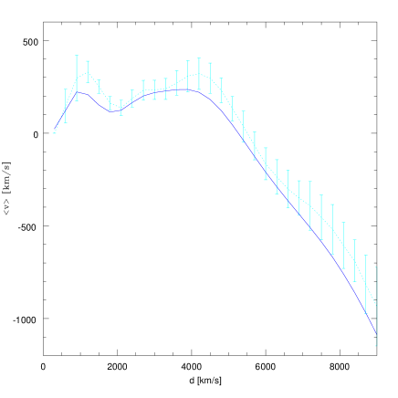
Figure 4: Mean radial velocities of shells according to models (solid line) and mock catalogs (dashed lines). Error bars correspond to fluctuations arising from different observers in the simulations.

Figure 5: occurrence of values $P_{0}$ and $\sigma_{TF}$ in random resamplings of a mock catalog with $\sigma_{TF}=0.41$ and $P_{0}=-0.05$

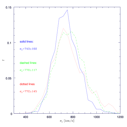
Figure 6: Probability distribution of $\sigma_{v}$ corresponding to mock catalogs with $\sigma_{TF}=0.3$ and $P_{0}=0$ (solid lines), $\sigma_{TF}=0.41$ and $P_{0}=-0.05$ (dashed lines), and $\sigma_{TF}=0.4$ and $P_{0}=-0.2$ (doted lines).

Observational errors in galaxy distance estimates were considered assuming gaussian errors in the galaxy absolute magnitudes of the TF relation with dispersion $\sigma_{TF}$, corresponding to relative errors in distances $\frac{\Delta d}{d}\simeq\frac{\sigma_{TF}}{2}$. Namely, we assign to each particle in the mock catalog a new distance $d_{new}=d(1+s)$ where $s$ is taken from a gaussian distribution with dispersion corresponding to the TF uncertainty. Then, as the particle peculiar velocities are inferred from the galaxy redshift and distance, $v_{new}=v-d\ s$.

The N-body numerical simulation was performed using the Adaptative Particle-Particle Particle-Mesh (AP3M) code developed by Couchman (1991). The initial condition was generated using the Zeldovich approximation and corresponds to the adiabatic CDM power spectrum with $\Omega=0.5$ and $\Omega_{\Lambda}=0$. We have adopted the analytic fit to the CDM power spectrum given by Sugiyama (1995):

$$P(k)\propto\frac{k}{A}\left(\frac{ln(1+2.34q)}{2.34q}\right)^{2}$$ (9)

where $A=[+3.89q+(16.1q)^{2}+(5.46q)^{3}+(6.71q)^{4}]^{1/2}$, $q=\frac{k}{\Gamma h}$Mpc, $\Gamma=\frac{k\theta^{2}}{h\ exp(-\Omega_{B}-\sqrt{h/0.5}\Omega_{B}/\Omega)}$, $\theta$ is the microwave background radiation temperature in units of $2.7K$, and $\Omega_{B}=0.0125h^{-2}$ is the value of the baryon density parameter given by nucleosynthesis. The normalization of the CDM power spectrum is imposed by COBE measurements using the value of $\sigma_{8}$ and $h$ (the Hubble constant in units of $100$ $km/s/Mpc$) chosen from Table 1 of Gorski et al. (1995) corresponding to an age of the universe $t_{0}\simeq$ 12 Gyr. The computational volume is a periodic cube of side length 300 Mpc. We have followed the evolution of $N=5\times 10^{5}$ particles with a $64^{3}$ grid and a maximum level of refinements of 4. The resulting mass per particle is $2.05\times 10^{12}h^{-1}M_{\sun}$. The initial condition corresponds to redshift $z=10$ and the evolution was followed using 1000 steps. At the final step ($z=0$) the linear extrapolated value of $\sigma_{8}$ is compatible with the normalization imposed by observed temperature fluctuations in the cosmic background.

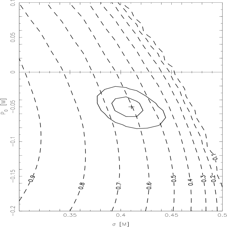
Figure 7: Probability contours corresponding to the observational sample $d<6000km/s$. Dashed lines corresponding to different values of $\beta$. The plus sign indicates the best values of $\sigma$ and $P_{0}$.

As a test of the ability of equation 7 to reproduce the distorted values of mean velocity, we plot in figure 4 the resulting $v^{\prime}_{a}$ for the average of 1000 mock catalogs, each with distance uncertaintes included. The error bars correspond to the rms deviation of $v^{\prime}$ from the different observers in the numerical simulation. We adopt the values of $\sigma_{TF}$ and $P_{0}$ used in the construction of the mock catalogs to perform the calculation of $v^{\prime}_{a}$ through equation 7. It can be seen in the figure the excellent agreement between the results of the calculation and the mock catalogs. We have applied a $\chi^{2}$ method to derive $\sigma_{TF}$ and $P_{0}$. We find that our method gives accurate estimates of the actual $\sigma_{TF}$ and $P_{0}$ when applied to the mock catalogs. In figure 5 we show the frequency of $\sigma_{TF}$ and $P_{0}$ obtained from bootstrap resampling objects corresponding to a mock catalog with an imposed scatter $\sigma_{TF}=0.4$ and $P_{0}=-0.05$ as derived from the observations.

The values of $\sigma_{TF}$ and $P_{0}$ inferred from the $\chi^{2}$ method can be used to calculate the value of $\sigma_{v}$ in the mock catalog through equation 8. The distributions of inferred $\sigma_{v}$ found are shown in figure 6 where it can be appreciated the stability of the method in estimating $\sigma_{1dim}$ under different zero-point offsets $P_{0}$ and $\sigma_{TF}$. The actual value of the rms peculiar velocity of the simulation is $\sigma_{v}\simeq 780$ $km/s$ which may be compared to the inferred values from equation 8 for different adopted values of $\sigma_{TF}$ and $P_{0}$. For instance, we find $\sigma_{v}=(743\pm 102)$ $km/s$, $\sigma_{v}=(770\pm 117)$ $km/s$, and $\sigma_{v}=(772\pm 145)$ $km/s$ for $\sigma_{TF}=0.3$, $P_{0}=0$; $\sigma_{TF}=0.41$, $P_{0}=-0.05$; and $\sigma_{TF}=0.4$, $P_{0}=-0.2$ respectively indicating the ability of our procedure to derive the rms peculiar velocity irrespectively of TF scatter and zero-point offset.

We find a zero-point shift $P_{0}=-0.05$ in our analysis of the observations using inverse TF distances. It is of interest to test the probability of occurrence of such a value arising from our model assumptions such as $v_{a}=0$, etc. We use mock catalogs with imposed $\sigma=0.4$ and $P_{0}=0$ in the TF calibration and we test the probability of finding different values of zero-point shifts . We apply a $\chi^{2}$ method to derive the pair of values $\sigma_{TF}$ and $P_{0}$ that provides the best-fitting of equation 7 to the actual values for each mock catalog. We compute the frequency of occurrence of $\sigma_{TF}$ and $P_{0}$ for the difference observers, and we can estimate the probability of obtaining different values of zero-point shifts. We find that a random occurrence of the observed value $P_{0}=-0.05$ is within a standard deviation, consistent with Willick et al. (1997) estimate.

6 DETERMINATION OF THE $\beta$ PARAMETER

The 3-dimensional velocity dispersion $\sigma_{v}$ is directly related to the quantity $\beta=\Omega^{0.6}/b$ through the relation [Peebles, 1980]

$$\sigma_{v}=\left(\frac{Haf}{b}\right)^{2}\int_{0}^{\infty}y\xi(y)dy$$ (10)

where $H$ is the Hubble constant, $a$ is the expansion factor of the universe, $y$ is expressed in $Mpc$, $\xi(y)$ the galaxy spatial correlation function, $f\simeq\Omega^{0.6}$ the rate of growth of inhomogeneities, and $b$ is the linear bias factor. We express $y$ in units of $Mpc$ $h^{-1}$, therefore $H=100km/s/Mpc$ and $a=1$.

We estimate $\Omega^{0.6}/b$ from the inferred value of 3-dimensional root mean square peculiar velocity. We adopt the power-law fit to the galaxy spatial correlation function estimated by Ratcliffe et al. (1997):

$$\xi(r)=\left\{\begin{array}[]{ll}(\frac{r}{r_{0}})^{-\gamma}&\mbox{if $r\leq 50$ $Mpc$}\\ 0&\mbox{if $r>50$ $Mpc$}\end{array}\right.$$

with $r_{0}=5.1$ $Mpc$ and $\gamma=1.6$.

We calculate $\beta$ from equation 10 using equation 8 to express $\sigma_{v}$ and therefore $\beta$ in terms of the parameters $\sigma_{TF}$ and $P_{0}$. In figure 7 we show equal $\beta$ contours in the $\sigma-P_{0}$ plane for our sample of Mark III spirals with distances $d<6000$ $km/s$. Also shown in this figure are the 1 $\sigma$ and 2 $\sigma$ contour levels corresponding to the frequency of inferred $\sigma_{TF}$ and $P_{0}$ from bootstrap resamplings of the observational data set. The corresponding result is $\beta=0.60^{+0.08}_{-0.05}$.

The true uncertainty of the global value $\beta=\Omega^{0.6}/b$ derived from a catalog of peculiar velocities will be grater than that obtained from bootstrap resampling of the data due to cosmic variance. A suitable value of the uncertainty in $\beta$ can be estimated from the rms values of this parameter derived from the mock catalogs. According to our analysis $\Delta\beta\simeq 0.1$ for a limiting distance $d_{max}<6000$. Thus, adding in quadrature both errors, we find $\beta=0.60^{+0.13}_{-0.11}$ for $d<6000km/s$.

Thus, the observed peculiar velocity field is inconsistent with a critical density universe if optical galaxies trace the mass.

7 CONCLUSIONS

We have developed a method for the analysis of the peculiar velocity field inferred from peculiar velocity data and we apply this procedure to the spirals of the Mark III catalog. We estimate optimal values of inverse Tully-Fisher scatter and zero-point offset for a sample of the catalog with limiting distance $d_{l}im=6000km/s$. We derive the 3-dimensional rms peculiar velocity of the galaxies $\sigma_{v}=(660\pm 50)km/s$ where the uncertainty has been obtained through bootstrap resampling of the data.

In our model, the shells have not a net mean radial motion, and the mean square velocities of galaxies in different shells are described by a unique number $\sigma_{v}$. The comparison with mock catalogs derived from numerical simulations shows that these are reasonable hypotheses that allow to obtain physical characterizations of the nearby universe from observations. We have shown that corrected TF distances require a large $P_{0}\simeq-0.15mag$ so that caution should be taken when they are used in statistical analysis.

We use mock catalogs derived from numerical simulations of CDM models considering measurement uncertainties and sampling variations to check our statistical analysis. We find a general good agreement between the results of the calculations and those measured in the mock catalogs. The spread of $\sigma_{v}$ measurements from different observers in the numerical simulations may be added in quadrature to the bootstrap resampling errors to provide a more reliable estimate of the uncertainty in $\sigma_{v}$. We infer $\sigma_{v}=660\pm 70$ $km/s$, and we conclude that $\beta\simeq\Omega^{0.6}/b=0.60^{+0.13}_{-0.11}$.

Estimates of the parameter $\beta$ from other analysis such as studies of redshift space distortions of the galaxy two point correlation function provide similar values $\beta\simeq 0.5$ (Ratcliffe et al. 1997). Moreover, the confrontation of observed cluster abundances with prediction of different cosmological models put constraints of the form $\Omega^{\alpha}/b\simeq 0.4-0.6$, values consistent with our determinations.

8 ACKNOWLEDGEMENTS

We have benefitted from helpful discussions with Jim Peebles and David Valls-Gabaud. This work was supported by the Consejo de Investigaciones Científicas y Técnicas de la República Argentina, CONICET, the Consejo de Investigaciones Científicas y Tecnológicas de la Provincia de Córdoba, CONICOR, and Fundación Antorchas, Argentina.

References

- [Barrow (1984)] Barrow J.D., Bhavsar S.P., Sonoda D.H. 1984, MNRAS, 210, 19P.