RECONSTRUCTION ANALYSIS OF THE IRAS POINT SOURCE CATALOG REDSHIFT SURVEY

Abstract

We present the results of reconstruction analysis of the galaxy distribution in a spherical region of radius $50{h^{-1}\;{\rm Mpc}}$ centered on the Local Group, as mapped by the IRAS Point Source Catalog Redshift Survey (PSCz). We reconstruct this galaxy distribution using 15 different models for structure formation in the universe, each model consisting of a set of assumptions regarding the value of the cosmological mass density parameter $\Omega_{m}$, and the amplitude and nature of the biasing between IRAS galaxies and the underlying mass. For every model, we also reconstruct ten mock PSCz catalogs derived from the outputs of numerical simulations that have the appropriate values of $\Omega_{m}$ and bias. We quantify the accuracy of a reconstruction using a variety of statistics and compare the accuracy of each reconstruction of the PSCz catalog to the accuracy expected based on the mock catalog reconstructions of the corresponding model. We find that gravitational instability of Gaussian primordial mass density fluctuations can account for the galaxy distribution in the PSCz catalog, at least for some plausible assumptions about the value of $\Omega_{m}$ and the biasing between IRAS galaxies and mass. However, unbiased models in which IRAS galaxies trace mass fail to reconstruct the PSCz catalog accurately, both for $\Omega_{m}=0.4$ and for $\Omega_{m}=1$. Low $\Omega_{m}$ models in which IRAS galaxies are antibiased with respect to the mass distribution are the most successful in reconstructing the PSCz catalog. In particular, a model with $\Omega_{m}=0.4$ and IRAS galaxies related to the mass distribution according to the predictions of a semi-analytic galaxy formation model is very successful in reproducing the properties of the PSCz galaxy distribution.

1 Introduction

Understanding the formation and evolution of large scale structure (hereafter LSS) in the universe is one of the foremost problems in cosmology. In the standard approach to studying LSS, one starts with a model for the primordial mass density fluctuations, uses analytical approximations or numerical simulations to predict the ensemble averaged statistical properties of galaxy clustering, and compares them with those of the observed galaxy distribution, assuming that we observe fair sample of the universe. However, we cannot expect a simulation started from random initial conditions to reproduce the specific structures observed in a galaxy redshift catalog, even if the statistical properties of the galaxy clustering are correct. Reconstruction analysis is a complementary approach to the study of LSS in which one works backward from the observed galaxy distribution to the initial mass density fluctuations in the same region of space, then evolves these model initial conditions forward in time to the present day using an N-body code. The reconstruction method incorporates assumptions about the properties of primordial fluctuations, the values of cosmological parameters, and the “bias” between the galaxy and mass distributions. These assumptions can be tested by comparing in detail the evolved reconstruction to the original galaxy redshift data. A by-product of the reconstruction analysis is a detailed model for the origin and evolution of familiar, well studied structures in the local universe, such as the Great Attractor, the Perseus-Pisces supercluster, and the Sculptor Void.

In this paper, we present the results of reconstruction analysis of the IRAS Point Source Catalog Redshift survey (hereafter PSCz, Saunders et al. 1995; Canavezes et al. 1998), using the “hybrid” reconstruction method described by Narayanan & Weinberg (1998, hereafter NW98). First, we create the galaxy density field smoothed with a Gaussian filter of radius $R_{s}=4{h^{-1}\;{\rm Mpc}}$ (where $h\equiv H_{0}/100\;{\rm\;km\;s^{-1}}\;{\rm Mpc}^{-1}$), correct for the effects of bias and redshift-space distortions, and derive the smoothed initial mass density field by tracing the evolution of these density fluctuations backward in time. We then evolve these initial density fluctuations forward using an N-body code, assuming a value for $\Omega_{m}$, and compare in detail the clustering properties of the reconstructed PSCz galaxy distribution to those of the input PSCz galaxy distribution, either assuming that galaxies trace mass or selecting galaxies from the N-body particle distribution using a biasing prescription. For our purposes, therefore, a model of structure formation consists of a value of $\Omega_{m}$, a bias factor $b$ that gives the ratio of rms galaxy and mass fluctuations on a scale of $8{h^{-1}\;{\rm Mpc}}$, and an explicit biasing scheme that specifies how galaxies are to be selected from the large scale mass distribution. All of our models assume that structure grew by gravitational instability from Gaussian primordial fluctuations — these are the implicit assumptions of the reconstruction method itself. We reconstruct the PSCz catalog using 15 different models and quantify the accuracy of each reconstruction using a variety of clustering statistics. Even if the model assumptions are correct, we do not expect to reproduce the observed structure exactly, because we begin with imperfect data and because the reconstruction method cannot invert gravitational evolution in the strongly non-linear regime. For each statistic, we therefore rank the accuracy of the model’s PSCz reconstruction with respect to the reconstructions of ten mock PSCz catalogs derived from the outputs of N-body simulations of the model under consideration. Finally, we use these ranks to evaluate the success of the PSCz reconstruction for each model, to constrain $\Omega_{m}$, and to test models of bias between the mass and IRAS galaxy distributions in the real universe.

The hybrid reconstruction technique (NW98) that we use for our PSCz analysis combines the complementary desirable features of the Gaussianization mapping method (Weinberg 1992), which assumes Gaussian primordial fluctuations and a monotonic relation between the smoothed initial mass density field and the smoothed final galaxy density field, and the dynamical reconstruction methods of Nusser & Dekel (1992) and Gramann (1993a), which are based on the momentum and mass conservation equations, respectively, under the approximation that the comoving trajectories of mass particles are straight lines (the Zel’dovich [1970] approximation). In the hybrid method, we first recover the smoothed initial density field from the smoothed final mass density field using a modified form of the dynamical methods, then Gaussianize this recovered initial density field to robustly recover the initial fluctuations even in the non-linear regions (an approach also used by Kolatt et al. 1996). For a reconstruction that incorporates biased galaxy formation, we precede the dynamical reconstruction step with a step that maps the smoothed galaxy density field monotonically to a smoothed mass density field with the theoretically expected (non-linear, non-Gaussian) PDF. The hybrid method is described and tested in detail in NW98, who show that it can reconstruct a galaxy redshift survey more accurately than either the Gaussianization method or the dynamical reconstruction methods alone. Comparison of the hybrid method to a variety of alternative reconstruction schemes, including the Path Interchange Zel’dovich Approximation (PIZA) method of Croft & Gaztañaga (1997), is given by Narayanan & Croft (1999).

Earlier attempts to reconstruct observational data include the reconstruction of the Perseus-Pisces redshift survey of Giovanelli & Haynes (1989) by Weinberg (1989) using the Gaussianization technique and the reconstruction of the IRAS $1.2$Jy redshift survey (Fisher et al. (1995)) by Kolatt et al. (1996) using the dynamical scheme of Nusser & Dekel (1992). This dynamical scheme was also used by Nusser, Dekel & Yahil (1995) to recover the PDF of the initial density field from the IRAS $1.2$Jy redshift survey. The primary requirements for a redshift survey to be suitable for reconstruction analysis are: (a) good sky coverage and depth, so that the gravitational influence of regions outside the survey boundaries is small, (b) dense sampling to reduce shot noise errors, and (c) a well understood selection function, to allow accurate construction of the observed galaxy density field. With respect to these criteria, PSCz is a substantial improvement on samples used in previous analyses, and it is the best all-sky redshift survey that exists today. The PSCz is a redshift survey of all galaxies in the IRAS Point Source Catalog whose flux at $60\ \mu m$ is greater than $0.6$Jy. It contains about $15,500$ galaxies distributed over $84.1\%$ of the sky, excluding only some regions of low Galactic latitude where the extinction in the $V$ band as estimated from the IRAS $100\ \mu m$ background is greater than 1.5 mag. (mainly the low Galactic latitude zone $|b|<5^{\circ}$), the Magellanic clouds, some odd patches contaminated by Galactic cirrus, and two strips in ecliptic longitude not surveyed by the IRAS satellite.

The plan of this paper is as follows. In §2, we describe the hybrid reconstruction method used to reconstruct galaxy redshift surveys, outline the assumptions involved in the reconstruction analysis, and list all the steps involved in reconstructing the PSCz catalog in the order in which they are implemented. In §3, we describe the various models that we use to reconstruct the PSCz catalog, and our construction of the mock PSCz catalogs for each model from the outputs of N-body simulations. In §4, we illustrate the results of reconstruction analysis for 6 of our 15 models, using a variety of statistics. We quantify the accuracy of the PSCz reconstruction of a model using a “Figure-of-Merit” for each statistic, and rank the PSCz reconstruction with respect to all the mock catalogs for that model. We summarize the results of reconstructing the PSCz catalog for the full set of 15 models in §5, and describe the criteria for classifying a model as Accepted, or Rejected, based on its rankings. We review our results and discuss their implications in §6, drawing general conclusions about the value of $\Omega_{m}$, the amplitude of mass density fluctuations, the bias between IRAS galaxies and mass, and the viability of gravitational instability with Gaussian initial conditions as an explanation for the structure observed in the PSCz redshift survey. A brief overview of our results can be obtained from Figures 3, 7, and 13, and Table 2.

2 Reconstruction Analysis

We reconstruct the galaxy distribution in the PSCz catalog using the “hybrid” reconstruction method of NW98. We refer the reader to NW98 for a detailed discussion of the method, including its general motivation and tests of its accuracy on N-body simulations. Here we provide a summary of the assumptions made in the reconstruction (§2.1), justification of our choice of smoothing length and sample radius for PSCz (§2.2), and a step-by-step description of the reconstruction procedure as applied to PSCz (§2.3).

2.1 Assumptions

Reconstruction analysis of a galaxy redshift catalog incorporates a number of assumptions, at various stages. These include assumptions about the cosmological parameters, about the nature of the primordial mass density fluctuations, about the process of structure formation, and about the physics of galaxy formation. The assumptions in our analysis are:

(1):

Structure formed by gravitational instability. The reconstruction procedure traces the evolution of density fluctuations backward in time under the assumption that the LSS formed from the gravitational instability of small amplitude fluctuations in the primordial mass density field. This assumption is also implicit when the power-restored initial density field is evolved forward in time using a gravitational N-body code.

(2):

The primordial density fluctuations form a Gaussian random field, as predicted by simple inflationary models for the origin of these fluctuations (Guth & Pi (1982); Hawking (1982); Starobinsky (1982); Bardeen, Steinhardt, & Turner 1983). This assumption is the basis of the Gaussianization step of the reconstruction procedure.

(3):

The values of $\Omega_{m}$ and the bias factor $b\equiv\sigma_{8g}/\sigma_{8m}$, where $\sigma_{8m}\ (\sigma_{8g})$ is the rms fluctuation of the mass (IRAS galaxy) distribution in spheres of radius $8{h^{-1}\;{\rm Mpc}}$. We vary these assumptions from one reconstruction to another. We use the value of $\Omega_{m}$ in correcting for redshift-space distortions and in forward evolution of the reconstructed initial conditions. We use the value of $\sigma_{8m}=\sigma_{8g}/b$ to normalize the forward evolution simulations. Note that throughout the paper we use $b$ to refer to the rms fluctuation bias on the $8{h^{-1}\;{\rm Mpc}}$ scale.

(4):

The shape of the primordial power spectrum. In contrast to the amplitude $\sigma_{8m}$, changes to the power spectrum shape make little difference to our results, because the shape is used only to compute corrections to or extrapolations of the initial power spectrum recovered from the observational data.

(5):

The evolved galaxy density field is a monotonic function of the evolved mass density field, once both are smoothed over scales of a few ${h^{-1}\;{\rm Mpc}}$. This assumption, together with the value of $\sigma_{8m}$ and the assumption of Gaussian initial conditions, allows us to recover the smoothed mass density field from the smoothed galaxy density field in preparation for the time-reversed dynamical evolution.

(6):

An explicit biasing scheme, i.e., a prescription for relating the underlying mass distribution to the observable galaxy distribution. This scheme does not influence the recovery of initial conditions, but it is needed to select galaxies from the N-body simulation evolved from these initial conditions, and hence to compare the reconstruction to the input data. Most of our biasing schemes have a single free parameter that controls the strength of the bias. We set the value of this parameter to obtain the desired bias factor $b$ (assumption 3).

2.2 Choice of smoothing length and sample radius

Since the PSCz is a flux-limited survey, the number density of galaxies in the catalog decreases with distance from the observer. Consequently, the shot-noise in the PSCz galaxy distribution increases with distance. However, the Gaussianization procedure in the reconstruction analysis relies on the assumption that the rms amplitude of galaxy density fluctuations remains the same throughout the reconstruction volume and that the contribution to these fluctuations from shot-noise in the galaxy distribution is negligible. In order to ensure that the shot-noise remains small and does not increase with distance from the observer, we create a volume-limited PSCz sub-catalog in which the number density of galaxies remains constant throughout the reconstruction volume.

Much of the diagnostic power of the reconstruction analysis stems from the fact that non-linear gravitational evolution transfers power from large scales to small scales (Melott & Shandarin (1990); Beacom et al. (1991); Little, Weinberg, & Park 1991; Soda & Suto (1992); Bagla & Padmanabhan (1997)). This power transfer erases the information about the initial mass fluctuations on scales below the non-linear scale (Fourier wavenumbers $k\geq k_{\rm nl}$). Consequently, a reconstruction method that recovers the initial fluctuations accurately up to the non-linear scale $k=k_{\rm nl}$ can reproduce many features of the evolved structures even on smaller scales $(k>k_{\rm nl})$, though not, of course, the finer details of these features. Since the rms fluctuation of the IRAS galaxy distribution in spheres of radius $8{h^{-1}\;{\rm Mpc}}$ is about 0.7 (Saunders, Rowan-Robinson & Lawrence 1992; Fisher et al. (1994); Moore et al. (1994)), we need to recover the initial density field accurately at least up to this scale in order to take advantage of the power-transfer phenomenon. We will therefore reconstruct the PSCz catalog using a Gaussian smoothing length of $R_{s}=4{h^{-1}\;{\rm Mpc}}$, which corresponds to a top-hat smoothing scale of about $6.6{h^{-1}\;{\rm Mpc}}$.

We create the volume-limited sub-catalog by selecting all the galaxies in the PSCz located within a volume-limiting radius that are bright enough to be included in the survey even when they are located at this volume-limiting radius. We choose this volume-limiting radius, $R_{1}$, based on a compromise between two conflicting requirements. First, the reconstruction volume should be large enough that it contains many independent smoothing volumes. This criterion pushes us to choose a large value for $R_{1}$. Second, the shot-noise in the galaxy distribution of the volume-limited catalog should be small and remain constant with distance from the observer. This condition requires a uniformly high number density of galaxies, pushing us to adopt a smaller volume-limiting radius. Since we reconstruct the PSCz catalog using a Gaussian smoothing length of $R_{s}=4{h^{-1}\;{\rm Mpc}}$, we fix $R_{1}$ so that the mean inter-galaxy separation at $R_{1}$ is $\bar{d}\equiv n_{g}^{-1/3}=\sqrt{2}R_{s}=5.6{h^{-1}\;{\rm Mpc}}$. We adopt this criterion $\bar{d}=\sqrt{2}R_{s}$ based on the rule of thumb suggested by Weinberg, Gott, & Melott (1987), to obtain the largest possible reconstruction volume while keeping shot-noise in the galaxy distribution small enough to have little effect on the smoothed galaxy density field.

We compute the number density of galaxies as a function of the distance from the observer in the PSCz catalog using the maximum-likelihood method described by Springel & White (1998). We find that the number density of galaxies drops to $0.005\ {\rm h^{3}Mpc^{-3}}=(5.6{h^{-1}\;{\rm Mpc}})^{-1/3}$ at a distance of $R_{1}=50{h^{-1}\;{\rm Mpc}}$ from the observer. We then select all the galaxies in the PSCz catalog that are bright enough to be included in the survey even if they are placed at a distance of $50{h^{-1}\;{\rm Mpc}}$ from the Local Group. The galaxies selected in this manner are then included in the PSCz sub-catalog, which is thus volume-limited to $R_{1}=50{h^{-1}\;{\rm Mpc}}$. The luminosities at $60\ \mu m$ of the galaxies in this sub-catalog satisfy the condition $\log_{10}\left(\frac{L_{60}}{L_{\odot}}\right)>9.37$ (for $h=1$).

2.3 Step-by-step description

The steps involved in reconstructing a $50{h^{-1}\;{\rm Mpc}}$, volume-limited subset of the PSCz catalog for a given set of model assumptions are as follows:
Step 1: Create an all-sky galaxy distribution by “cloning” the galaxy distribution to fill in the regions excluded in the PSCz survey. The PSCz catalog does not include galaxies in regions of low Galactic latitude where there is substantial obscuration by dust. However, this region could be dynamically important, since the Perseus-Pisces supercluster and the Hydra-Centaurus supercluster are both located close to the Galactic plane and could even extend across it. Hence, we fill in the region with Galactic latitude $|b_{\rm cut}|<8^{\circ}$, using the cloning technique introduced by Lynden-Bell, Lahav & Burstein (1989; see also Yahil et al. 1991). We divide this region into 36 angular bins of $10^{\circ}$ in longitude and divide the redshift range in each angular bin into bins of $1000{\rm\;km\;s^{-1}}$. In each longitude-redshift bin, we assign $N(l,z)$ artificial galaxies, where $N(l,z)$ is equal to a random Poisson deviate whose expectation value is equal to the average density of the corresponding longitude-redshift bins in the adjacent strips $|b_{\rm cut}|<|b|<2|b_{\rm cut}|$, times the volume of the bin. If there is a real PSCz galaxy in any of these longitude-redshift bins, we include it in place of an artificial galaxy. We fill the masked regions at high Galactic latitudes with a random distribution of artificial galaxies having the observed mean density. The flux distribution of the artificial galaxies is identical to those of the real galaxies in the PSCz catalog. We tested (using mock PSCz catalogs) alternate methods of handling the mask region, including assigning galaxies at random locations within the mask region at the mean galaxy density, as well as ignoring all the galaxies in the mask region. We found that the cloning technique always leads to the most accurate reconstruction of the galaxy distribution. However, the mask region does not influence reconstruction analysis as much as it influences say, the analysis of the cosmological galaxy dipole (Rowan-Robinson et al. in preparation).
Step 2: Select a volume-limited galaxy distribution from the flux-limited PSCz catalog so that the shot-noise in the volume-limited catalog is small and remains constant throughout the reconstruction volume. Based on the selection function of the PSCz survey, we choose the volume-limiting radius $R_{1}=50{h^{-1}\;{\rm Mpc}}$, where the mean inter-galaxy separation is $\bar{d}=\sqrt{2}R_{s}=5.6{h^{-1}\;{\rm Mpc}}$.
Step 3: Compute the smoothed galaxy density field in redshift space. We create the PSCz galaxy density field in redshift space by cloud-in-cell (CIC) binning (Hockney & Eastwood 1981) the volume-limited galaxy distribution onto a $100^{3}$ cubical grid that represents $200{h^{-1}\;{\rm Mpc}}$ on a side. The Local Group observer is at the center of this cube, and the three sides of the cube are oriented along the axes of the Supergalactic coordinate system. Since the dynamical component of the hybrid reconstruction method traces the evolution of the gravitational potential backward in time, it is necessary to model the gravitational field in the regions beyond the boundaries in order to reconstruct the density field accurately near the edges of the volume-limited catalog. We therefore supplement the volume-limited density field with the density field in an annular region $20{h^{-1}\;{\rm Mpc}}$ thick beyond the volume-limiting radius of $50{h^{-1}\;{\rm Mpc}}$. We form the density field in this annular region by weighting each galaxy by the inverse of the selection function of the flux-limited PSCz survey at the location of the galaxy. The full galaxy density field is therefore constructed from a volume-limited catalog in the region $0<R<R_{1}=50{h^{-1}\;{\rm Mpc}}$ and from a flux-limited catalog in the region $R_{1}<R<R_{2}=70{h^{-1}\;{\rm Mpc}}$. We fill the regions beyond $R_{2}$ with uniform density equal to the mean density of the galaxy distribution in the volume-limited catalog, $n=0.005\ {\rm h^{3}Mpc^{-3}}$. We smooth the galaxy density field using a Gaussian filter of radius $R_{s}=4{h^{-1}\;{\rm Mpc}}$. We account for boundary effects in computing the smoothed density field $\rho_{sm}({\bf r})$ by using the ratio smoothing method of Melott & Dominik (1993),

$$\rho_{sm}({\bf r})=\frac{\int M({\bf r^{\prime}})\rho({\bf r^{\prime}})W({\bf r-r^{\prime}})d^{3}{\bf r^{\prime}}}{\int M({\bf r^{\prime}})W({\bf r-r^{\prime}})d^{3}{\bf r^{\prime}}},$$ (1)

where $W({\bf r})$ is the smoothing filter, and the mask array $M({\bf r})$ is set to 1 for pixels inside the survey region and to 0 for pixels outside the survey region. The rms amplitude of the galaxy density field smoothed with a Gaussian filter of radius $R_{s}=4{h^{-1}\;{\rm Mpc}}$ is $\sigma_{4G}=0.85$.
Step 4: Monotonically map the galaxy density field onto a theoretically determined PDF of the underlying mass distribution. In an unbiased model, the galaxy density field is identical to the mass density field, so we skip this step entirely. In a biased model, we derive the mass density field using the PDF mapping procedure described in NW98. We first assume a value for the bias factor $b$ and estimate the rms linear mass fluctuation using the equation

$$\sigma_{8m}=\frac{\sigma_{8g}}{b},$$ (2)

where $\sigma_{8g}$ and $\sigma_{8m}$ are the rms fluctuations in $8h^{-1}$Mpc spheres in the non-linear galaxy density field and the linear mass density field, respectively. We use an N-body code to evolve forward in time an ensemble of initial mass density fields, all drawn from the same assumed power spectrum, and all normalized to this value of $\sigma_{8m}$. We then derive an ensemble-averaged PDF of the smoothed final mass density fields from the evolved mass distributions of these simulations. While reconstructing the PSCz catalog using a model that corresponds to this value of $\sigma_{8m}$, we derive a smoothed final mass density field by monotonically mapping the smoothed PSCz galaxy density field to this average PDF. This step implicitly derives and corrects for the only monotonic local biasing relation that is simultaneously consistent with the observed galaxy PDF, the assumed shape of the power spectrum and value of $b$, and the assumption of Gaussian initial conditions.
Step 5: Correct for the effects of redshift-space distortions. The peculiar velocities of galaxies distort the mapping of galaxy positions from real space to redshift space, making the line-of-sight a preferred direction in an otherwise isotropic universe. Since we need the real space mass density field to recover the initial mass density fluctuations, we need to correct for these redshift-space distortions. On small scales, the velocity dispersion of a cluster stretches it along the line-of-sight into a “Finger of God” feature that points directly toward the observer (e.g., de Lapparent, Geller & Huchra (1986)), thereby reducing the amplitude of small-scale clustering. To correct for this effect, we first identify the clusters in redshift space using a friends-of-friends algorithm that uses a transverse linking length of $0.6{h^{-1}\;{\rm Mpc}}$ and a radial linking length of $500{\rm\;km\;s^{-1}}$ (Huchra & Geller (1982); Nolthenius & White (1987); Moore, Frenk, & White 1993; Gramann, Cen, & Gott 1994). For each cluster, we then shift the radial locations of its member galaxies so that the resulting compressed cluster has a radial velocity dispersion of $100{\rm\;km\;s^{-1}}$, roughly the value expected from Hubble flow across its radial extent. On large scales, the distortions arise from coherent inflows into overdense regions and outflows from underdense regions (Sargent & Turner (1977); Kaiser (1987)). To remove these distortions, we apply the following iterative procedure, which is a modified version of the method suggested by Yahil et al. (1991) and Gramann et al. (1994). This method is described in detail in NW98, and we give only a brief outline here. After deriving the mass density field in step (4), we predict the velocity field using the second order perturbation theory relation (Gramann 1993b ),

$${\bf v(r)}=f(\Omega_{m})H\left[{\bf g(r)}+\frac{4}{7}\nabla C_{g}({\bf r})\right],$$ (3)

where ${\bf g(r)}$ is the gravitational acceleration field computed from the equation $\nabla\cdot{\bf g(r)}=-\delta_{m}({\bf r})$ and $C_{g}$ is the solution of the Poisson type equation

$$\nabla^{2}C_{g}=\sum_{i=1}^{i=3}\sum_{j=i+1}^{j=3}\left[{\partial^{2}\phi_{g}\over\partial x_{i}^{2}}{\partial^{2}\phi_{g}\over\partial x_{j}^{2}}-{\left(\partial^{2}\phi_{g}\over\partial x_{i}\partial x_{j}\right)^{2}}\right].$$ (4)

Equation (3) requires that we assume a value of $\Omega_{m}$, to compute the factor $f(\Omega_{m})\approx\Omega_{m}^{0.6}$ (Peebles (1980)). Finally, we correct the positions of galaxies so that their new positions are consistent with their Hubble flow and the peculiar velocities at their new locations. We repeat these three steps until the corrections to the galaxy positions become negligible, which usually occurs within 3 iterations.
Step 6: Apply the dynamical reconstruction scheme to evolve the fluctuations backward in time. We compute the gravitational potential from this smoothed mass density field using the Poisson equation, then evolve this gravitational potential backward in time using our modified version of the Gramann (1993) method. We use Poisson equation to derive the initial mass density fluctuations i.e., the fluctuations that grow according to the predictions of linear theory.
Step 7: Gaussianize this dynamically reconstructed initial mass density field. This step enforces a Gaussian PDF for the initial mass density fluctuations and yields robust reconstructions even in the non-linear regions.
Step 8: Restore power to the recovered initial density field. Non-linear gravitational evolution tends to suppress the small-scale power in the reconstructed density field, beyond the suppression due to the Gaussian smoothing alone. We correct for this effect using the “power restoration” procedure described in Weinberg (1992). Using an ensemble of numerical simulations, we compute a set of correction factors $C(k)$ defined by

$$C(k)=\left[\frac{P_{r}(k)}{P_{i}(k)}\right]^{1/2}~{},$$ (5)

where $P_{i}(k)$ is the power spectrum of a simulation’s smoothed initial conditions, and $P_{r}(k)$ is the power spectrum of the density field recovered by the hybrid reconstruction method. We multiply each Fourier mode of the reconstructed density field by $C(k)$ and also multiply by $\exp(k^{2}R_{s}^{2}/2)$ in order to remove the effect of the original Gaussian smoothing. Above some wavenumber $k_{\rm corr}\approx\pi/R_{\rm nl}$, where $R_{\rm nl}$ is the scale on which the rms fluctuations are unity, non-linear evolution erases the information about the phases in the initial density field (Little et al. (1991); Ryden & Gramann (1991)) to the point that the hybrid method cannot recover it. For $k_{\rm corr}<k\leq k_{\rm Nyq}$, therefore, we add random phase Fourier modes with an assumed shape for the power spectrum, where $k_{\rm Nyq}$ is the Nyquist frequency of the grid on which we define the density fields. We normalize this power spectrum by fitting it to the power spectrum of the recovered initial density field in the range of wavenumbers $k_{1}\leq k\leq k_{2}$, where $k_{1}$ and $k_{2}$ are wavenumbers in the linear regime, with $k_{1}<k_{2}\leq k_{\rm corr}$. In the range of wavenumbers $k_{2}<k\leq k_{\rm corr}$, multiplication by the large factor $\exp(k^{2}R_{s}^{2}/2)$ can distort the shape of the power spectrum, although this range of wavenumbers is only in the mildly non-linear regime. In this range of Fourier modes, therefore, we preserve the phases of the recovered initial density field but fix the amplitude of the modes to be that determined by the fitting procedure. In all of our simulations, $k_{\rm Nyq}=50k_{f}$, and we choose $k_{\rm corr}=15k_{f}$, $k_{1}=4k_{f}$ and $k_{2}=8k_{f}$, where $k_{f}=2\pi/L_{\rm box}=0.0314\ h$Mpc^-1 is the fundamental frequency of the simulation box. We assume that the shape of the power spectrum is governed by the parameter $\Gamma$, which is equal to $\Omega_{m}h$ in cold dark matter models with small baryon fraction and scale-invariant inflationary fluctuations (Efstathiou, Bond, & White, 1992). We do not add the small scale power using the technique of constrained realizations (Bertschinger (1987); Hoffman & Ribak (1991); van de Weygaert & Bertschinger (1996)) because we find it does not lead to a more accurate reconstruction even for a dense sampling of the constraints (see NW98 for a more detailed discussion).
Step 9: Evolve the power-restored density field forward in time using an N-body code. We evolve the reconstructed initial mass distribution using a particle-mesh (PM) code, assuming the values of $\Omega_{m}$ and $\Omega_{\Lambda}$. This code is described and tested in Park (1990). We use $100^{3}$ particles and a $200^{3}$ force mesh in the PM simulations. We start the gravitational evolution from a redshift $z=23$ and follow it to $z=0$ in 46 equal incremental steps of the expansion scale factor $a(t)$. We fix the amplitude of the linear mass density fluctuations to be $\sigma_{8m}=\sigma_{8g}/b$, where $b$ is the bias factor. In the case of truly unbiased models (as opposed to biased models with $b=1.0$), we instead fix the amplitude of the linear mass fluctuations by requiring that the non-linear rms amplitude of fluctuations in redshift space smoothed with a Gaussian filter of radius $4{h^{-1}\;{\rm Mpc}}$ ($\sigma_{4G,g}$) from the simulation match the observed value.
Step 10: Compare the evolved distribution with the original galaxy distribution, either assuming that galaxies trace mass or using a local biasing model to select galaxies from the mass distribution. In biased reconstructions, we choose the free parameter controlling the strength of the bias by requiring that the rms fluctuation $\sigma_{4G}$ of the reconstructed, redshift-space galaxy density field, smoothed with a Gaussian filter of radius $4{h^{-1}\;{\rm Mpc}}$, match that of the original galaxy density field.

Figure 1 illustrates the intermediate steps in a hybrid reconstruction analysis of the PSCz catalog. Panel (a) shows the redshift-space positions of all galaxies in the volume-limited PSCz catalog, in a slice $30{h^{-1}\;{\rm Mpc}}$ thick centered on the Supergalactic plane (SGP). Panel (b) shows a slice through the SGP of the galaxy density field smoothed with a $4{h^{-1}\;{\rm Mpc}}$ Gaussian filter. The smoothed initial density field recovered by the hybrid reconstruction method is shown in panel (c). The mass distribution obtained by evolving the power-restored initial mass density field using an N-body code is shown in panel (d). The reconstructed, smoothed, redshift-space galaxy density field, and the reconstructed, redshift-space galaxy distribution obtained by selecting galaxies from the evolved mass distribution using a power-law biasing model (see §3.1 below) are shown in panels (e) and (f), respectively. The reconstruction illustrated in Figure 1 assumes $\Omega_{m}=0.4$, $\Omega_{\Lambda}=0.6$, and $b=0.64$.

Figure 1: Steps in the reconstruction analysis of PSCz catalog. (a) The observed PSCz galaxy distribution, (b) the observed PSCz galaxy density field, (c) the initial mass density field linearly extrapolated to the present epoch, (d) the reconstructed mass distribution, (e) the reconstructed PSCz galaxy density field, and (f) the reconstructed PSCz galaxy distribution. The contour plots show the density field in the Supergalactic plane, smoothed with a Gaussian filter of radius $R_{\rm s}=4{h^{-1}\;{\rm Mpc}}$. Solid contours correspond to regions above the mean density $\bar{\rho}$ and are in steps of 0.1 in $\log(\rho/\bar{\rho})$, while dashed contours correspond to regions below the mean density and are in steps of $0.2$ in $(\rho/\bar{\rho})$. The galaxy distributions show all the galaxies in redshift space in a slice $30h^{-1}$Mpc thick centered on the Supergalactic plane, and volume limited to a radius $R_{1}=50{h^{-1}\;{\rm Mpc}}$. This reconstruction corresponds to the model L4PLb0.64 listed in Table 1.

3 PSCz Reconstruction: Models and Mock Catalogs

3.1 Model Assumptions

We use 15 different models to reconstruct the PSCz catalog and to create mock catalogs for calibrating reconstruction errors. Each model consists of a set of assumptions regarding the values of $\Omega_{m}$ and $\Omega_{\Lambda}$, the shape of the linear mass power spectrum $P(k)$ as characterized by the parameter $\Gamma$ described in step (8) of §2.3, the bias factor $b$ defined as $b=b_{8}=\sigma_{8g}/\sigma_{8m}$, and the functional form of the biasing relation between IRAS galaxies and the underlying dark matter distribution. As discussed in §2.3, these assumptions influence the reconstruction analysis in different ways. The value of $\Omega_{m}$ is required when we correct the input data for redshift-space distortions and when we evolve the power-restored initial conditions forward in time. The shape ($\Gamma$) and amplitude ($\sigma_{8m}=\sigma_{8g}/b$) of the mass power spectrum are used to calculate the correction factors $C(k)$, and the shape is used to extrapolate the recovered initial power spectrum above the wavenumber $k>k_{\rm corr}$. The value of the bias factor $b$ is required when we map the biased galaxy density field to the numerically determined PDF of the underlying mass density field with rms fluctuation amplitude $\sigma_{8m}=\sigma_{8g}/b$. It is also required in the forward evolution step when we evolve the power-restored initial mass density field to match the rms fluctuation amplitude $\sigma_{8m}$. We need to assume an explicit biasing scheme to select galaxies from the evolved mass distribution. Most of our biasing schemes have one free parameter that we fix so that the rms fluctuation of the resulting galaxy distribution matches that of the input galaxy distribution, and a random sampling factor that we use to match the number density of galaxies in our volume-limited PSCz sample.

Our models span a wide range of cosmological and galaxy formation parameters, varying with respect to the following properties:

(1):

$\Omega_{m}$ and $\Omega_{\Lambda}$: Our assumptions for the geometry of the background universe include Einstein de-Sitter models $(\Omega_{m}=1.0,\ \Omega_{\Lambda}=0)$, open models $(\Omega_{m}<1.0,\ \Omega_{\Lambda}=0)$, and flat models with a non-zero cosmological constant $(\Omega_{m}<1.0,\ \Omega_{m}+\Omega_{\Lambda}=1.0)$.

(2):

Normalization and shape of the power spectrum: We normalize the amplitude of the primordial mass density fluctuations (characterized by $\sigma_{8m}$) either to be consistent with the level of anisotropies in the cosmic microwave background measured by the COBE satellite (the COBE normalization, Smoot et al. (1992)) or to produce the observed abundance of clusters at the present epoch (the cluster normalization, White, Efstathiou & Frenk 1993; Eke, Cole & Frenk 1996; Viana & Liddle (1996)). For all cluster-normalized models, we choose the values of $\Omega_{m}$ and $\sigma_{8m}$ so that $\sigma_{8m}\Omega_{m}^{0.6}=0.55$ (White et al. (1993)), for both open and flat universes. We refer the reader to Cole et al. (1997) and Cole et al. (1998, hereafter CHWF98) for more details of the COBE and cluster normalization procedures. We define the shape parameter of the transfer function in the linear mass power spectrum via the parameter $\Gamma$ of Efstathiou et al. (1992); for CDM models with low baryon content, $\Gamma\approx\Omega_{m}h$. Our power spectra include scale-invariant $(n=1)$ models with $\Gamma$ values consistent with the clustering properties measured from several galaxy catalogs, viz., $\Gamma=0.15-0.3$ (Maddox et al. (1990); Efstathiou et al. (1992); Vogeley et al. (1992); Peacock & Dodds (1994); Gaztañaga, Croft, & Dalton 1995; Maddox, Efstathiou, & Sutherland 1996; Gaztañaga & Baugh (1998); Tadros, Efstathiou, & Dalton 1998), and some models with larger $\Gamma$ values. We also consider power spectra that are normalized to both the COBE and cluster constraints, by introducing a tilt in the spectral index of the power spectrum. Finally, two of our models are not normalized to COBE or clusters, although the rms fluctuation of the reconstructed galaxy distributions matches that of the IRAS galaxies.

(3):

Bias factor: We consider models in which IRAS galaxies trace mass (unbiased, $b=1.0$), models in which IRAS galaxies are more strongly clustered than the mass (biased, $b>1.0$), and models in which galaxies are more weakly clustered than the mass (antibiased, $b<1.0$). We even consider one biasing model in which the galaxies do not trace mass but $b=1.0$, i.e., the rms amplitude of fluctuations in the galaxy and mass distributions are identical at the scale of $8{h^{-1}\;{\rm Mpc}}$, but the galaxy density has a non-linear dependence on the mass density.

(4):

Biasing scheme: Our biasing relations cover a wide range of plausible functional forms, with the only constraint being that they remain monotonic. These include functions derived empirically from observations of different types of galaxies, functions predicted from semi-analytic models of galaxy formation, functions that fit the results of numerical studies of galaxy formation, and functions constructed ad-hoc. All of our biasing models are deterministic, and are “local” in the sense that the efficiency of galaxy formation is determined by the properties of the local environment, i.e., by the properties within approximately one correlation length of the location of the galaxy. We compute all the local properties of the mass distribution in a sphere of radius $4{h^{-1}\;{\rm Mpc}}$ centered on the galaxy.

The specific biasing schemes that we use to select the IRAS galaxies from the evolved mass distributions of our reconstructions are as follows.
Power-law bias: In this simple biasing model, the IRAS galaxy density ($\rho_{g}$) is a steadily increasing, power-law function of the local mass density, $(\rho_{g}/{\overline{\rho}}_{g})\propto(\rho_{m}/{\overline{\rho}}_{m})^{B}$. The probability for an N-body particle with local mass density $\rho_{m}$ to be selected as an IRAS galaxy is therefore

$$P=A(\rho_{m}/{\overline{\rho}}_{m})^{B-1}.$$ (6)

We choose the values of $A$ and $B$ to reproduce the required number density and the rms fluctuation of the resulting galaxy distribution, respectively. This biasing relation is similar to the one suggested by Cen & Ostriker (1993) based on hydrodynamic simulations incorporating physical models for galaxy formation (Cen & Ostriker (1992)), but it differs in that there is no quadratic term that saturates the biasing relation at high mass densities.
Threshold bias: In this biasing scheme, galaxy formation is entirely suppressed below some threshold value of mass density, and IRAS galaxies form with equal efficiency per unit mass in all regions above the threshold. This biasing scheme was adopted in some of the early numerical investigations of CDM models (e.g., Melott & Fry (1986)), and it has been used extensively in theoretical modeling of voids and superclusters (e.g., Einasto et al. (1994)). In the density-threshold bias model, the probability that a particle with local mass density $\rho_{m}$ is selected as an IRAS galaxy is

$$P=\cases{A&if $\rho_{m}\geq B,$\cr 0&if $\rho_{m}<B$.\cr}$$ (7)

We choose the threshold density $B$ to match the required bias factor $b$, and the probability $A$ to reproduce the desired galaxy number density. We note that, since this model preferentially populates regions of higher mass density, it can only lead to a bias factor greater than unity, and hence cannot be used when an antibias ($b<1.0$) is required.
Morphology-density bias: It has been known for a long time that early-type galaxies are preferentially found in dense environments, while late-type galaxies dominate in less massive groups and in the field (Hubble (1936); Zwicky (1937); Abell (1958)). There have been numerous efforts to quantify this connection between morphology and environment (e.g., Dressler (1980); Postman & Geller (1984); Lahav & Saslaw (1992); Whitmore, Gilmore, & Jones (1993)), using a variety of clustering statistics including angular correlation functions, redshift-space correlation functions, and de-projected real-space correlation functions (Davis & Geller (1976); Giovanelli, Haynes & Chincarini (1986); Loveday et al. (1995); Hermit et al. (1996); Guzzo et al. (1997); Willmer et al. (1998)). We model the “bias” arising from this morphological segregation using the morphology-density relation proposed by Postman & Geller (1984). Since the IRAS-selected galaxy catalogs preferentially include dusty, late-type spirals (Soifer et al. (1984); Meiksin & Davis (1986); Lawrence et al. (1986); Babul & Postman (1990)), we select all the spiral galaxies as IRAS galaxies. The morphology-density relation of Postman & Geller (1984) assigns morphological types to galaxies based on the densities at the locations of all the galaxies. Since we evolve the power-restored density field forward in time using a low resolution PM code and with a finite number of mass particles, the final densities computed over spheres centered on the galaxies and large enough to contain significant numbers of neighbors will be different from the densities at the exact locations of the galaxies. Therefore, we recast the morphology-density relation of Postman & Geller (1984) in terms of the density computed in a sphere of radius $2{h^{-1}\;{\rm Mpc}}$ centered on the galaxy. We assign the galaxy a spiral (Sp), S0, or elliptical (E) morphological type, with relative probabilities $F_{\rm Sp}$, $F_{\rm S0}$, and $F_{\rm E}$ that depend on the density computed within a sphere of radius $2{h^{-1}\;{\rm Mpc}}$. For $\rho<\rho_{F}=10{\overline{\rho}}$, the morphological fractions are $F_{\rm Sp}=0.7$, $F_{\rm S0}=0.2$, and $F_{\rm E}=0.1$. For $\rho_{F}<\rho<\rho_{C}=6\times 10^{3}{\overline{\rho}}$, the fractions are

$$F_{\rm Sp} = 0.7-0.2\alpha$$

$$F_{\rm E} = 0.1+0.1\alpha$$ (8)

$$F_{\rm S0} = 1-F_{\rm Sp}-F_{\rm E}$$

$$\alpha = \log_{10}(\rho/\rho_{F})/\log_{10}(\rho_{C}/\rho_{F}).$$

For $\rho>\rho_{C}$, the morphological fractions saturate at $F_{\rm Sp}=0.5$, $F_{\rm S0}=0.3$, and $F_{\rm E}=0.2$. The ratio of rms fluctuations in $8{h^{-1}\;{\rm Mpc}}$ spheres of the elliptical and spiral galaxy distributions selected in this manner is 1.3, consistent with the ratio of $\sim 1.2-1.7$ observed between optical and IRAS galaxy distributions (Lahav, Nemiroff, & Piran 1990; Strauss et al. (1992); Saunders et al. (1992); Peacock & Dodds (1994); Willmer, da Costa, & Pellegrini 1998; Baker et al. (1998)). This biasing scheme has no free parameters, so the resulting bias factor is known a priori.
Square-root Exponential bias: We construct a biasing scheme in which the IRAS galaxy density field is related to the mass density field by

$$y=A\sqrt{x}\exp(\alpha x),$$ (9)

where $x=\rho_{m}/{\overline{\rho}}_{m}$ and $y=\rho_{g}/{\overline{\rho}}_{g}$ are the mass and the IRAS galaxy overdensities, respectively. We choose the values of $\alpha$ and $A$ to reproduce the required galaxy rms fluctuation and the mean number density, respectively. This biasing relation is a monotonically increasing function for all $\alpha>0$. We include this ad-hoc biasing scheme to test the ability of reconstruction analysis to distinguish between different biasing relations with the same bias factor. We use this biasing scheme in a model in which galaxies do not trace the mass, although $b=1.0$. We note that neither the Power-law bias nor the Threshold bias can lead to $b=1.0$, for any non-trivial values of the free parameters governing the strength of the bias.
Semi-analytic bias: Except for the connection between power-law bias and the simulations of Cen & Ostriker (1993), the biasing models described so far are not based on theoretical models of the galaxy formation process. Rather, they include a variety of reasonable functional forms that could plausibly represent the results of some more complete theory of biased galaxy formation. We now consider a biasing scheme that is motivated by a physical theory of galaxy formation namely, the semi-analytic galaxy formation model of Benson et al. (1999; see also Cole et al. 1994, 1999). We parameterize this biasing scheme as follows. We consider the luminosities and morphologies of all the galaxies selected by Benson et al. (1999) from the mass distribution of the $\Lambda$CDM2 simulation of Jenkins et al. (1998, the VIRGO consortium). We select as IRAS galaxies all the galaxies whose ratio of bulge to total mass is less than $0.4$. The rms fluctuation of the IRAS galaxy distribution selected in this manner ($\sigma_{8g}$), is about $10\%$ smaller than that of the underlying mass distribution.

The solid points in Figure 2 show the mean relation between this “IRAS” galaxy density field and the underlying mass density field, after both fields are smoothed with a top-hat filter of radius $R_{\rm th}=3{h^{-1}\;{\rm Mpc}}$. The thick solid line shows an empirical fit to this mean relation using a smoothly varying double power-law of the form

$$y=Ax^{\alpha}\left[C+x^{(\alpha-\beta)/\gamma}\right]^{-\gamma},$$ (10)

where $\alpha=2.9$, $\beta=0.825$, $\gamma=0.4$, $C=0.08$, $A=1.1$, and $x=(1+\delta_{m})$, $y=(1+\delta_{g})$ are the mass and the IRAS galaxy overdensities, respectively, smoothed with a top-hat filter of radius $R_{\rm th}=3{h^{-1}\;{\rm Mpc}}$. During the reconstruction analysis, we use this semi-analytic biasing relation to select the IRAS galaxies from the evolved mass distribution. We found that the scatter around this mean relation is dominated by shot-noise and hence ignore it in our parameterization of the semi-analytic bias model. This bias model does not have any free parameters, so it results in a known bias factor. Note that this relation was derived for a $\Lambda$CDM model with $\sigma_{8m}=0.9$, although we apply it here to an open model with slightly lower $\sigma_{8m}$ so that it matches the $\sigma_{8g}$ of IRAS galaxies.

Figure 2: The mean relation between the IRAS galaxy overdensity, $\rho_{g}/{\overline{\rho}}_{g}=(1+\delta_{g})$, and the mass overdensity, $\rho_{m}/{\overline{\rho}}_{m}=(1+\delta_{m})$, in the Semi-analytic galaxy formation model. Both the density fields are smoothed with a top-hat filter of radius $R_{\rm th}=3{h^{-1}\;{\rm Mpc}}$. The solid points show the mean relation obtained from the simulation of Benson et al. (1999), while the thick solid line shows the empirical fit to it using a smoothly varying double power law, described by equation (10). The dotted line shows the relation $\rho_{g}/{\overline{\rho}}_{g}=\rho_{m}/{\overline{\rho}}_{m}$, corresponding to an unbiased model in which galaxies trace mass.

3.2 Models

The 15 different models that we analyze in this paper sample the range of interesting values of the parameters $\Omega_{m}$ and $\sigma_{8m}$ (or, equivalently, the bias factor $b$). Thus, we analyze models with $\Omega_{m}=0.2,0.3,0.4,0.5,$ and $1.0$, while the values of $\sigma_{8m}$ range from $0.4$ to $1.44$. The parameters of all these models are listed in Table 1. In our model nomenclature, the first two symbols denote the geometry of the universe and the value of the cosmological mass density parameter. Thus, E1 represents an Einstein de-Sitter model with $\Omega_{m}=1.0,\ \Omega_{\Lambda}=0$; Ox represents an open model with $\Omega_{m}=0.{\rm x},\ \Omega_{\Lambda}=0$; and Lx represents a flat model with $\Omega_{m}=0.{\rm x}$ and a cosmological constant $\Omega_{\Lambda}=1-\Omega_{m}$. The capital letters immediately following specify the nature of the local biasing relation between the IRAS galaxy distribution and the underlying mass distribution. The last series of numbers after the letter $b$ corresponds to the bias factor of the model. For example, the model O4SQEb1.0 specifies an open model with $\Omega_{m}=0.4$ in which the biasing relation is a square-root exponential function and the bias factor is 1.0.

We now briefly describe the features of all the 15 models. In §4, we will illustrate our analysis methods and results using 6 representative models, before giving summary results for the full suite of 15 models in §5. The 6 illustrative models are:
E1UNb1.0 — An Einstein de-Sitter universe, in which IRAS galaxies trace the mass distribution (unbiased), and hence $b=1.0$. The shape of the power-spectrum is consistent with the observed clustering of galaxies, $\Gamma=0.25$ (Peacock & Dodds (1994)). The mass normalization agrees with the measured value of $\sigma_{8g}\approx 0.7$ for this biasing model, but it is above the cluster normalization constraint $\sigma_{8m}=0.55$ for $\Omega_{m}=1$.
E1PLb1.8 — An Einstein de-Sitter universe, in which there is a power-law biasing relation between the IRAS galaxy and mass distributions. We choose the value of $B$ so that $b=1.8$ and the value of $A$ so that $n_{g}=0.005h^{3}$Mpc^-3. The mass fluctuation amplitude is below the level $\sigma_{8m}=0.55$ implied by cluster normalization or by COBE normalization for its adopted $\Omega_{m}$ and shape of the power spectrum. It requires a large value of the bias factor ($b=1.8$) to match the rms fluctuation of the IRAS galaxies. This model has $\Gamma=0.25$ and a tilted power spectrum with $n=0.803$; it is similar to the E2(tilted) model of Cole et al. (1998), except that the rms fluctuation amplitude is $\sigma_{8m}=0.40$ instead of 0.55.
O4MDb0.7 — An open universe with $\Omega_{m}=0.4$ and $\Omega_{\Lambda}=0$, in which the galaxy population as a whole traces the mass distribution. We select the IRAS galaxies using the morphology-density biasing relation. This model is cluster-normalized, and it requires the IRAS galaxies to be antibiased with respect to the mass, i.e., $b<1.0$.
O4SAb0.9 — An open universe with $\Omega_{m}=0.4$ and $\Omega_{\Lambda}=0$, in which the galaxies are selected from the mass distribution using the semi-analytic biasing model. Although this model is COBE-normalized by construction, it can simultaneously reproduce the observed mass function of clusters (Cole et al. (1997)).
O4SQEb1.0 — An open universe with $\Omega_{m}=0.4$ and $\Omega_{\Lambda}=0$, in which the IRAS galaxy density field is related to the mass density field by the square-root exponential biasing function. We choose the value of $\alpha=0.041$ so that $b=1.0$ and the value of $A$ so that $n_{g}=0.005h^{3}$Mpc^-3. In this model, the IRAS galaxies do not trace the mass distribution even though the bias factor $b=1.0$. The parameters of this model are similar to those of O4SAb0.9, except that the biasing relation is very different.
L3PLb0.62 — A flat universe with $\Omega_{m}=0.3$ and $\Omega_{\Lambda}=0.7$, in which the bias between galaxies and mass is described by the power-law bias model. This model is COBE-normalized, and it requires the IRAS galaxies to be antibiased with respect to the mass distribution. It can also reproduce the observed abundance of clusters at the present epoch (Cole et al. (1997)).

We also reconstructed the PSCz catalog using another set of 9 models, which, together with the 6 models described above, extend our exploration of the $\Omega_{m}$, $\sigma_{8m}$ parameter space. These 9 models are all either cluster-normalized, or COBE-normalized, or both. They are:
E1PLb1.3 — An Einstein de-Sitter universe, in which the probability for a mass particle with local mass density $\rho_{m}$ to become a galaxy is given by the power-law biasing relation. We choose the value of $B$ so that $b=1.3$ and the value of $A$ so that $n_{g}=0.005h^{3}$Mpc^-3. This model is both cluster-normalized and COBE-normalized, and it has a tilted power spectrum with $n=0.803$ and $\Gamma=0.451$.
E1PLMDb1.3 — An Einstein de-Sitter universe, in which the galaxy population as a whole is biased using a power-law function. We choose the value of $B$ so that $\sigma_{8g}\approx 1.0$. We then use the morphology-density relation to select all the spiral galaxies as IRAS galaxies, so that $\sigma_{8g}\approx 0.7$. The resulting bias factor of IRAS galaxies is $b\approx 1.3$. This model has the same mass power spectrum as E1PLb1.3.
E1THb1.3 — An Einstein de-Sitter universe, in which we select the galaxies from the mass distribution using the threshold biasing relation. We choose the threshold density $B$ so that the bias factor $b=1.3$, and the probability $A$ so that the mean galaxy density is $n_{g}=0.005{h^{3}\;{\rm Mpc}^{-3}}$. This model has the same mass power spectrum as E1PLb1.3.
O2PLb0.5 — An open universe with $\Omega_{m}=0.2$ and $\Omega_{\Lambda}=0$, in which the IRAS galaxies are selected from the mass distribution using the power-law biasing relation. This model is cluster-normalized, and it has the largest amplitude of mass fluctuations ($\sigma_{8m}=1.44$) among all of our 15 models.
O3PLb1.4 — An open universe with $\Omega_{m}=0.3$ and $\Omega_{\Lambda}=0$, in which the IRAS galaxies are selected from the mass distribution using the power-law biasing relation. This is a COBE-normalized model.
O4UNb1.0 — An open universe with $\Omega_{m}=0.4$ and $\Omega_{\Lambda}=0$, in which the IRAS galaxies trace the mass distribution. Although this model is COBE-normalized by construction, it can simultaneously reproduce the observed mass function of galaxy clusters (Cole et al. (1997)).
L2PLb0.77 — A flat universe with $\Omega_{m}=0.2$ and $\Omega_{\Lambda}=0.8$, in which there is a power-law biasing relation between the IRAS galaxies and the mass. This model is COBE-normalized, and it requires the IRAS galaxies to be antibiased with respect to the mass.
L4PLb0.64 — A flat universe with $\Omega_{m}=0.4$ and $\Omega_{\Lambda}=0.6$, in which there is a power-law biasing relation between the IRAS galaxies and the mass. This model is COBE-normalized, and it requires the IRAS galaxies to be antibiased with respect to the mass. This model can simultaneously reproduce the observed mass function of clusters (Cole et al. (1997)).
L5PLb0.54: A flat universe with $\Omega_{m}=0.5$ and $\Omega_{\Lambda}=0.5$, in which there is a power-law biasing relation between the IRAS galaxies and the mass. This model is also COBE-normalized, and it requires a strong antibias between the IRAS galaxies and the mass.

Table 1: Parameters of the 15 models used to reconstruct the PSCz survey. For each model, columns 1 to 7 list the name of the model, the cosmological mass density parameter $\Omega_{m}$, the cosmological constant $\Omega_{\Lambda}$, the rms amplitude of the mass density fluctuations in $8{h^{-1}\;{\rm Mpc}}$ spheres $\sigma_{8m}$, the cluster normalization parameter $\sigma_{8m}\Omega_{m}^{0.6}$, the parameter $\beta_{\rm IRAS}=\Omega_{m}^{0.6}/b$ where $b=\sigma_{8\rm IRAS}/\sigma_{8m}$ is the bias parameter of IRAS galaxies, and the shape parameter $\Gamma$ that specifies the shape of the linear mass transfer function (Efstathiou et al. 1992). A Y (N) in column 8 shows that the model satisfies (does not satisfy) the cluster constraint, while a similar notation in column 9 shows whether the model is COBE normalized. Column 10 lists the type of local biasing model used to select the IRAS galaxies from the underlying mass distribution. The final column specifies the name of the simulation in CHWF98 from which we created the mock catalogs for each model.

							Normalization			Mock
Name	$\Omega_{m}$	$\Omega_{\Lambda}$	$\sigma_{\rm 8m}$	$\sigma_{\rm 8m}\Omega_{m}^{0.6}$	$\beta_{\rm IRAS}$	$\Gamma$	Cluster	COBE	Bias/Antibias	catalog
E1UNb1.0	1.0	0.0	0.70	0.70	1.00	0.250	N	N	Unbiased	E3S
E1PLb1.3	1.0	0.0	0.55	0.55	0.78	0.451	Y	Y	Power-law	E2
E1PLMDb1.3	1.0	0.0	0.55	0.55	0.78	0.451	Y	Y	Power-law/MD	E2
E1THb1.3	1.0	0.0	0.55	0.55	0.78	0.451	Y	Y	Threshold	E2
E1PLb1.8	1.0	0.0	0.40	0.40	0.57	0.451	N	N	Power-law	E2
O2PLb0.5	0.2	0.0	1.44	0.55	0.78	0.25	Y	N	Power-law	O2S
O3PLb1.4	0.3	0.0	0.5	0.24	0.34	0.172	N	Y	Power-law	O3
O4UNb1.0	0.4	0.0	0.75	0.43	0.61	0.234	N	Y	Unbiased	O4
O4MDb0.7	0.4	0.0	0.95	0.55	0.78	0.25	Y	N	Morph-den	O4S
O4SAb0.9	0.4	0.0	0.75	0.43	0.61	0.234	N	Y	Semi-analytic	O4
O4SQEb1.0	0.4	0.0	0.75	0.43	0.61	0.234	N	Y	Sq-Exp.	O4
L2PLb0.77	0.2	0.8	0.9	0.34	0.49	0.131	N	Y	Power-law	L2
L3PLb0.62	0.3	0.7	1.13	0.55	0.78	0.25	Y	N	Power-law	L3S
L4PLb0.64	0.4	0.6	1.1	0.63	0.90	0.213	N	Y	Power-law	L4
L5PLb0.54	0.5	0.5	1.3	0.86	1.23	0.27	N	Y	Power-law	L5

3.3 Mock Catalogs

If the reconstruction method were perfect, and structure in the universe really did form from gravitational instability of Gaussian initial conditions, then we would expect to reproduce exactly the galaxy distribution in the PSCz catalog, if we assumed the correct value of $\Omega_{m}$ and the correct biasing relation between IRAS galaxies and mass. However, the reconstruction method suffers from inaccuracies arising at various intermediate steps — inaccuracies in the bias mapping procedure, inaccuracies in correcting for the redshift-space distortions, inaccuracies in the dynamical recovery of the initial mass density fluctuations, and inaccuracies in the forward evolution step caused by poor modeling of the large scale tidal field and (on small scales) the finite numerical resolution. All these errors accumulate at various levels, with the result that we cannot expect a reconstruction to produce an exact match to the input data even if all of its assumptions are correct. It is therefore necessary to calibrate the magnitude of the errors intrinsic to the reconstruction method before we can derive any conclusions regarding the validity of the various assumptions entering the reconstruction procedure.

We assess these errors by reconstructing a set of mock PSCz catalogs for each of the 15 different models. For every model, we construct the mock PSCz catalogs from the outputs of numerical simulations that have the appropriate values of $\Omega_{m}$ and bias. The geometry, the sky-coverage, the depth, and the selection function of the mock catalogs all mimic those of the original PSCz catalog.

We construct the mock catalogs for 14 of the 15 models using the outputs of the N-body simulations of cold dark matter models performed by CHWF98. The CHWF98 simulations use a modified version of the AP3M code of Couchman (1991) to follow the gravitational evolution of $192^{3}$ particles in a periodic cubical box of side $345.6{h^{-1}\;{\rm Mpc}}$, using a gravitational softening length of $\epsilon=90{h^{-1}\;{\rm kpc}}$ (for a Plummer force law), fixed in comoving coordinates. Further details of the simulations are in CHWF98. For the model E1PLb1.8, we created the mass distribution by evolving an initial density field with parameters similar to the E2(tilted) model of CHWF98, except that $\sigma_{8m}=0.4$ instead of 0.55. We evolved $192^{3}$ particles on a $384^{3}$ force mesh using the PM code of Park (1990). Our goal here was to investigate an $\Omega_{m}=1.0$ model with lower mass fluctuation amplitude than those considered by CHWF98, which is why we needed to run a new simulation. For the other 14 models, the $90{h^{-1}\;{\rm kpc}}$ force resolution of the mock catalog simulation is much higher than the $\sim 1{h^{-1}\;{\rm Mpc}}$ force resolution of the PM simulation used in the forward evolution step of the reconstruction procedure. Our calibration of systematic errors therefore includes the error caused by limited force resolution of the PM simulations.

For every model (except E1PLb1.8), the last column in Table 1 lists the CHWF98 simulation from which we derive the mock catalogs. If the model involves bias, we start by selecting the galaxies from the mass distribution using the appropriate biasing algorithm. We then select “observers” from the galaxy distributions so that they satisfy the following observed properties of the Local Group:

(1):

The velocity of the Local Group observer should be in the range $550{\rm\;km\;s^{-1}}<V_{LG}<700{\rm\;km\;s^{-1}}$, consistent with the amplitude of the dipole anisotropy in the cosmic microwave background (Smoot et al. (1991)).

(2):

The overdensity of galaxies in a spherical region of radius $5{h^{-1}\;{\rm Mpc}}$ centered on the Local Group observer should be in the range $1.0<1+\delta_{g}(5{h^{-1}\;{\rm Mpc}})<2.0$ (Brown & Peebles (1987); Hudson (1993); Schlegel et al. (1994)).

(3):

The radial velocity dispersion in a sphere of radius $5{h^{-1}\;{\rm Mpc}}$ around the Local Group observer should be less than $150{\rm\;km\;s^{-1}}$, consistent with the observations of a cold velocity field near the Local Group (Sandage & Tammann (1975); Sandage (1986); Giraud (1986); Schlegel et al. (1994)). We note that for all but one of the galaxy distributions (corresponding to the E1UNb1.0 model), our Local Groups have local velocity dispersion smaller than $100{\rm\;km\;s^{-1}}$.

(4):

The Local Group particles for any pair of mock catalogs constructed from a simulation should be separated by at least $50{h^{-1}\;{\rm Mpc}}$. This criterion ensures that the density fields in the mock PSCz catalogs centered on these observers are quite different from each other, at least within the volume-limiting radius $R_{1}=50{h^{-1}\;{\rm Mpc}}$.

We assign each particle in the galaxy distribution a redshift based on its real space distance and its radial peculiar velocity with respect to the Local Group observer particle. We assign luminosities to these galaxies consistent with the luminosity function of the IRAS galaxies in the PSCz catalog. We “observe” this galaxy distribution using the selection function of the PSCz survey. We reject all the galaxies in the angular regions not covered by the PSCz catalog, so that the sky coverage in the mock catalogs is identical to that of the true PSCz catalog. We create 10 mock PSCz catalogs for each of the 15 models and reconstruct them in exactly the same manner as the PSCz catalog.

4 PSCz Reconstruction: Illustrative Results

We now describe the results of reconstructing the PSCz catalog and ten mock catalogs for the first 6 of the 15 models described in §3.2. Figure 3 shows a slice through the galaxy density fields of the true and the reconstructed PSCz catalogs. The density fields have been convolved with a Gaussian filter $e^{-r^{2}/2R_{s}^{2}}$, with smoothing radius $R_{s}=4h^{-1}$Mpc. The slices show the contours of the density field in the SGP. The galaxy density field traced by the galaxies in the PSCz catalog is shown in panel (a). Some of the prominent features include the Perseus-Pisces supercluster seen as the overdensity near the boundaries in the bottom right region, the Great Attractor region in the diagonally opposite direction near the top left corner, and the Local void in the bottom left region. We refer the reader to Branchini et al. (1999) for a detailed cosmographical description of the PSCz catalog. Panels (b) through (f) show the galaxy density fields reconstructed in the models E1UNb1.0, E1PLb1.8, O4MDb0.7, O4SAb0.9, and L3PLb0.62, respectively. All the models can, at least qualitatively, reproduce the general features of the observed PSCz galaxy distribution. This success offers support to the hypothesis that structure formed from the gravitational instability of Gaussian primordial mass density fluctuations. We will see below that, although the various reconstructions resemble the observed PSCz galaxy density field in this visual representation, there are quantifiable differences between the accuracy of the reconstructions corresponding to different models. Thus, some models (like, for example, the models O4MDb0.7, O4SAb0.9 and L3PLb0.62) can reconstruct the PSCz catalog as well as can be expected based on the mock catalog reconstructions, while others (including the models E1UNb1.0 and E1PLb1.8) fail in a systematic manner.

Figure 3: Contours in the Supergalactic plane in the true and reconstructed PSCz density fields. The density fields are smoothed with a Gaussian filter of radius $R_{s}=4h^{-1}$Mpc. Solid contours correspond to regions above the mean density $\bar{\rho}$ and are in steps of 0.1 in $\log(\rho/\bar{\rho})$, while dashed contours correspond to regions below the mean density and are in steps of $0.2$ in $(\rho/\bar{\rho})$. (a) The observed PSCz density field. Remaining panels show the density field reconstructed in the following models: (b) E1UNb1.0, (c) E1PLb1.8, (d) O4MDb0.7, (e) O4SAb0.9, and (f) L3PLb0.62.

Figure 4 shows the redshift-space locations of galaxies in the volume-limited PSCz catalog and its reconstructions. We plot the SGX and SGY coordinates of all the galaxies that lie in a slice $30h^{-1}$Mpc thick centered on the SGP. The different panels show the true PSCz galaxy distribution and the various reconstructions, in the same format as Figure 3.

Figure 4: Galaxy distributions in redshift space in the PSCz survey and its reconstructions. The panels show all the galaxies in a slice $30h^{-1}$Mpc thick centered on the Supergalactic plane, and volume limited to a radius $R_{1}=50{h^{-1}\;{\rm Mpc}}$. (a) The observed PSCz galaxy distribution. Remaining panels show the reconstructed galaxy distributions for the models listed in Fig. 1.

One of the most obvious quantitative measurements of the success of a reconstruction is the correlation coefficient $r$ between the original and the reconstructed smoothed galaxy density fields,

$$r\equiv\frac{\left<\delta_{r}\delta_{t}\right>}{\left<\delta_{r}^{2}\right>^{\frac{1}{2}}\left<\delta_{t}^{2}\right>^{\frac{1}{2}}},$$ (11)

where $\delta_{t}$ and $\delta_{r}$ are respectively the original and reconstructed smoothed galaxy density fields. Panels (a) through (f) of Figure 5 show the correlation coefficients for the models E1UNb1.0, E1PLb1.8, O4MDb0.7, O4SAb0.9, O4SQEb1.0, and L3PLb0.62, respectively. For every model, we assign ranks to the reconstructions of each of the 10 mock catalogs and to the reconstruction of the true PSCz catalog, in descending order of their values of $r$: the catalog whose reconstruction has the highest $r$ value is assigned a rank of 0, the catalog whose reconstruction has the lowest $r$ value is assigned a rank of 10, and so on in between. The solid line in each panel shows the values of $r$ for the 10 mock catalog reconstructions of the model, in rank order. The horizontal dashed line shows the value of $r$ for the PSCz reconstruction based on the model assumptions. We find that the absolute values of $r$ tend to decrease for models with larger values of $\sigma_{8m}$ (smaller values of $b$) because the greater degree of non-linear gravitational evolution makes the recovery of initial conditions less accurate. The absolute value of $r$ is therefore of little use for comparing the viability of different reconstruction models. We focus instead on the value of $r$ relative to the values expected given the model assumptions, and since the PSCz reconstructions for all six of these models have a rank of seven or less (and the models therefore reproduce PSCz better than they reproduce at least three of their own mock catalogs), we conclude that all of them are acceptable by this particular measure.

Figure 5: The correlation between the true and reconstructed smoothed galaxy density fields. The solid line in all the panels shows the distribution of the correlation coefficient (eq. 11) between the true and reconstructed smoothed galaxy density fields for the ten independent mock catalogs, while the dashed line shows the same quantity for the PSCz reconstruction. The different panels show the galaxy distributions reconstructed with the following assumptions: (a) E1UNb1.0, (b) E1PLb1.8, (c) O4MDb0.7, (d) O4SAb0.9, (e) O4SQEb1.0, and (f) L3PLb0.62. Note that the range of the vertical axis varies from one panel to another.

The correlation coefficient quantifies the success of the reconstruction in matching the observed galaxy density field at a particular scale, $R_{s}=4{h^{-1}\;{\rm Mpc}}$. In order to probe a range of scales, Figure 6 shows the distribution of the Fourier difference statistic

$$D(k)\equiv\frac{\sum|\tilde{\delta}_{r}({\bf k})-\tilde{\delta}_{t}({\bf k})|^{2}}{\sum\left(|\tilde{\delta}_{r}({\bf k})|^{2}+|\tilde{\delta}_{t}({\bf k})|^{2}\right)},$$ (12)

where the subscripts $t$ and $r$ refer to the true and reconstructed density fields respectively, and $\tilde{\delta}({\bf k})$ represents the complex Fourier component of the density field. The summation is over all the waves with $|{\bf k}|$ in the interval $\left(k-1,k\right]$. This statistic measures the difference in both the moduli and the phases of the Fourier components of the true and reconstructed density fields, and it is independent of any smoothing of the density fields. It was first used by Little et al. (1991) to demonstrate the effects of power-transfer from large scales to small scales during non-linear gravitational evolution. When the complex amplitudes of the Fourier components of the true and reconstructed density fields are identical, $D(k)=0$, while for two fields with uncorrelated phases, the average value of $D(k)=1$. Figure 6 shows the value of $D(k)$ averaged over the range of wavenumbers $k_{\rm surv}<k<k_{8}$, where $k_{\rm surv}=2\pi/(2\times R_{1})=0.0628\ h$Mpc^-1 is the wavenumber corresponding to the size of the reconstruction volume, and $k_{8}=2\pi/(2\times 8)=0.3927\ h$Mpc^-1 is the wavenumber corresponding to the length scale of $8{h^{-1}\;{\rm Mpc}}$, approximately equal to the scale of non-linearity in the PSCz galaxy distribution. The different panels correspond to the six models in the same format as Figure 5. The solid line in each panel shows the distribution of $D(k)$ in the ten mock catalog reconstructions of that model. The dashed line shows the value of $D(k)$ in the PSCz reconstruction. We rank the mock catalog reconstructions and the PSCz reconstruction, in ascending order of their values of $D(k)$. We find that the PSCz reconstruction has a high rank (of 9) in the model E1UNb1.0, and has smaller ranks in all the other models. Hence, the model E1UNb1.0 fails (though only at the $80\%$ confidence level) to reproduce the PSCz density field as measured by this statistic, while the other five models yield acceptable reconstructions.

Figure 6: The Fourier difference statistic $D(k)$ between the true and the reconstructed galaxy density fields (eq. 12). The solid line in all the panels shows the distribution of the value of $D(k)$ averaged over the range of wavenumbers $k_{\rm surv}<k<k_{8}$ in the ten independent mock catalogs, while the dashed line shows the same quantity for the PSCz reconstruction. The different panels correspond to the galaxy distributions reconstructed using the various models listed in Fig. 4. Note that the axis range varies from one panel to another.

Figure 7 shows the PDF of the true and reconstructed galaxy density fields for the six models. We compute the PDF of a density field after smoothing it with a Gaussian filter of radius $R_{s}=4{h^{-1}\;{\rm Mpc}}$. In every panel, the crosses and the thin solid line show the PDFs of the true and reconstructed galaxy density fields for a typical mock catalog — the one with rank $5$ according to the Figure-of-Merit (FOM) for this statistic, defined as the maximum value of the absolute difference between the cumulative distributions $C_{t}(\nu)$ and $C_{r}(\nu)$ of the true and reconstructed galaxy density fields,

$${\rm FOM}_{\rm PDF}={\rm max}\ |C_{t}(\nu)-C_{r}(\nu)|.$$ (13)

This is the FOM that would be used in a Kolmogorov-Smirnov comparison of the PDFs, and we find that it gives similar results in terms of ranks to a FOM based on absolute differences of the differential PDFs. The open circles and the thick solid line show the true and reconstructed PDFs for the PSCz reconstruction, offset vertically by 0.2 for the sake of clarity.

For every model, we rank the mock catalog reconstructions and the PSCz reconstruction, in increasing order of the FOM of the statistic. If the reconstruction of PSCz based on the model assumptions is worse than expected from the mock catalog tests, then the PSCz reconstruction will have a high rank. A low PSCz rank, conversely, implies a reconstruction that is successful given the expectations from the mock catalog tests. Visual comparison between the PDF recoveries for PSCz and for the rank-$5$ mock catalogs in Figure 7 suggests that the PSCz reconstructions for the models E1UNb1.0, E1PLb1.8, O4MDb0.7, and O4SQEb1.0 should have high ranks, while the PSCz reconstructions for the models O4SAb0.9 and L3PLb0.62 should have low ranks. This is indeed the case, as can be verified by the PSCz ranks listed in each panel.

We show the ranks for all other statistics in Figures 8 through 12, in the same format as in Figure 7 for the PDF statistic. If the PSCz catalog has a rank of 5 for any of the statistics, we show the results for the mock catalog ranked 6 according to that statistic. We will use the ranks for all the statistics as the basis for a more systematic evaluation of models in §5.

Figure 7: PDF of the true and reconstructed galaxy density fields. All the density fields are smoothed with a Gaussian filter of radius $R_{s}=4h^{-1}$Mpc. The crosses and the thin solid line show the PDFs of the true and reconstructed smoothed density fields of a mock catalog, the one with rank 5 according to the FOM for this statistic defined in equation (13). The open circles and the thick solid line show the same quantities for the PSCz catalog, and are vertically offset by 0.2 for clarity. The different panels correspond to the galaxy distributions reconstructed using the various models listed in Fig. 4. A successful model should reproduce the PSCz (i.e., show agreement between the circles and thick line) about as well as it reproduces its own mock catalogs (as illustrated for a typical case by the crosses and thin line). Each panel lists the rank of the PSCz reconstruction based on the model assumptions, relative to the reconstructions of the model mock catalogs, according to the FOM for this statistic.

Figure 8 shows the distribution of galaxy counts in spheres of radius $8{h^{-1}\;{\rm Mpc}}$, in the true and reconstructed galaxy distributions for the six models. We compute this distribution by placing $50,000$ spherical cells at random locations within the reconstruction volume and counting the number of galaxies within each cell. If a cell lies close to the boundary of the survey region, we include it in the distribution only if at least $90\%$ of its volume lies within the survey region. The crosses and the thin solid line show the distributions of counts in the true and reconstructed galaxy distributions of the mock catalog with rank 5. The open circles and the thick solid line show the same quantities for the PSCz catalog, and are vertically offset by 0.05 for clarity. We define the FOM for this statistic as

$${\rm FOM}_{\rm COUNTS}=\sum_{N=1}^{N=\infty}|P_{t}(N)-P_{r}(N)|,$$ (14)

where $P_{t}(N)$ and $P_{r}(N)$ are the distributions of the counts in cells in the true and reconstructed galaxy distributions. From visual inspection of Figure 8, we would expect the models E1UNb1.0, E1PLb1.8, and O4SQEb1.0 to have high ranks and the models O4MDb0.7, O4SAb0.9, and L3PLb0.62 to have low ranks, as is indeed verified by the ranks of the PSCz reconstruction listed in different panels. We also computed this distribution using spherical cells of radius $3{h^{-1}\;{\rm Mpc}}$, but do not show the corresponding figure. Although the distribution of galaxy counts is a measure similar to the PDF statistic shown in Figure 7, here we are using different smoothing filters (top-hat instead of Gaussian) and smoothing lengths ($3{h^{-1}\;{\rm Mpc}}$ and $8{h^{-1}\;{\rm Mpc}}$ instead of $4{h^{-1}\;{\rm Mpc}}$).

Figure 8: Distributions of galaxy counts in spheres of radius $8{h^{-1}\;{\rm Mpc}}$ in the true and reconstructed galaxy distributions. The crosses and the thin solid line show the counts in cells of the true and reconstructed galaxy distributions of the mock catalog ranked $5$ according to the FOM for this statistic (eq. 14). The open circles and the thick solid line show the same quantities for the PSCz catalog, and are vertically offset by 0.05 for clarity. The different panels correspond to the galaxy distributions reconstructed using the various models listed in Fig. 4.

Figure 9 shows the void probability function (VPF) in the true and reconstructed galaxy distributions for the six models. Like the PDF and the count distributions, this statistic is sensitive to higher-order correlations in the density field (White (1979); Balian & Schaeffer (1989); Sheth (1996)), and it can distinguish between biased and unbiased galaxy formation models (Little & Weinberg (1994)). The probability $P_{0}(R)$, that a randomly placed sphere of radius $R$ is devoid of galaxies is a subset of the more general count distribution statistic $P_{N}(R)$, but here we examine $P_{0}$ at a range of $R$ instead of $P_{N}$ at fixed $R=8{h^{-1}\;{\rm Mpc}}$, as in Figure 8. When computing the VPF, we require that at least $90\%$ of the spherical cell’s volume lie within the survey region. We define the FOM for this statistic as

$${\rm FOM}_{\rm VPF}=\sum_{R=0}^{R=\infty}|P_{0t}(R)-P_{0r}(R)|,$$ (15)

where $P_{0t}(R)$ and $P_{0r}(R)$ are the VPFs of the true and reconstructed galaxy distributions, and the sum extends over discrete bins in $R$. By visual comparison with the mock catalog reconstructions, we expect the models E1UNb1.0, E1PLb1.8, O4MDb0.7, and O4SQEb1.0 to have high ranks. This expectation is confirmed by the ranks of the PSCz reconstruction listed in each panel. We also computed the underdensity probability function (UPF) introduced by Weinberg & Cole (1992) and found that the different models have similar ranks for the UPF as for the VPF. The UPF requires that a sphere be more than $80\%$ below the mean density rather than completely empty.

Figure 9: Void probability functions (VPF) of the true and reconstructed galaxy distributions. The crosses and the thin solid line show the VPFs of the true and reconstructed galaxy distributions of the mock catalog ranked $5$ according to the FOM for this statistic (eq. 15). The open circles and the thick solid line show the same quantities for the PSCz catalog, and are vertically offset by 0.5 for clarity. The different panels correspond to the galaxy distributions reconstructed using the various models listed in Fig. 4.

Figure 10 shows the distribution of distances to nearest neighbors in the true and reconstructed catalogs. If computed in three dimensions using galaxy redshift distances, this statistic would show a spurious peak at neighbor separations corresponding to the velocity dispersions of typical galaxy groups. Therefore, we instead estimate the nearest-neighbor distribution from the redshift-space galaxy distributions using the method suggested by Weinberg & Cole (1992). For every galaxy at a redshift $z$, we consider all the galaxies that lie within a redshift range $\Delta v<1000\ {\rm kms^{-1}}$ to be its potential nearest neighbor. Of these candidate neighbors, we then choose the galaxy that lies closest to this galaxy in the transverse direction, and we compute the distribution of this transverse separation $R_{t}$ divided by the mean inter-galaxy separation $\bar{d}$ (i.e., $x_{n}=R_{t}/\bar{d}$). This approach biases the estimated neighbor distance, but the bias is the same for the PSCz data and the reconstructions. We define the FOM for this statistic as

$${\rm FOM}_{\rm NNBR}=\sum_{x_{n}=0}^{x_{n}=1}|P_{t}(x_{n})-P_{r}(x_{n})|,$$ (16)

where $P_{t}(x_{n})$ and $P_{r}(x_{n})$ are the nearest-neighbor distributions of the true and reconstructed galaxy distributions. From the ranks of the PSCz reconstruction in different panels, we find that the models E1PLb1.8 and O4SQEb1.0 have high ranks, while the other models have low ranks.

Figure 10: Distribution of distances to nearest neighbors in the true and reconstructed galaxy distributions. We compute this distribution from the redshift-space locations of galaxies using the method described in the text. The thin dashed and solid lines show the nearest neighbor distributions of the true and reconstructed galaxy distributions of the mock catalog ranked $5$ according to the FOM for this statistic (eq. 16). The thick dashed and solid lines show the same quantities for the PSCz catalog, and are vertically offset by 0.7 for clarity. The different panels correspond to the galaxy distributions reconstructed using the various models listed in Fig. 4.

Figure 11 shows the redshift-space correlation functions $\xi(s)$ for the true and reconstructed catalogs. We compute the correlation functions using the estimator of Hamilton (1993),

$$\xi(s)=\frac{N_{DD}N_{RR}}{N_{DR}^{2}}-1,$$ (17)

where $N_{DD},N_{DR}$, and $N_{RR}$ are the number of galaxy-galaxy, galaxy-random, and random-random pairs with a redshift-space separation $s$. We use a random catalog that has the same geometry and selection function as the PSCz catalog and contains 50,000 points distributed randomly within the survey volume. We consider only those galaxy pairs that subtend an angle smaller than $\alpha_{max}=60^{\circ}$ at the observer so that the lines of sight to both the galaxies in the pair are approximately parallel. We fit the correlation function in the region $1{h^{-1}\;{\rm Mpc}}<s<15{h^{-1}\;{\rm Mpc}}$ with a power-law of the form $\xi(s)=\left(\frac{s}{s_{0}}\right)^{\gamma}$, where $s_{0}$ is the redshift-space correlation length and $\gamma$ is the index of the power-law. We define the FOM as

$${\rm FOM}_{\xi}=|\gamma_{t}-\gamma_{r}|,$$ (18)

where $\gamma_{t}$ and $\gamma_{r}$ are the slopes of the true and reconstructed, redshift-space correlation functions. We find that the model E1UNb1.0 has a high rank, while the other five models have low ranks. The failure of the model E1UNb1.0 is the one expected if we reconstruct a low $\Omega_{m}$ universe using a high value of $\Omega_{m}$: the high velocity dispersion in an $\Omega_{m}=1$ model leads to excessive suppression of $\xi(s)$ on small scales, while the large amplitude of the coherent bulk motions (Kaiser (1987)) boosts it on large scales. Thus, the reconstructed $\xi(s)$ has a shallower slope compared to the true $\xi(s)$. We investigated a number of alternative FOM definitions, but we found (using the mock catalogs rather than the PSCz data set itself) that the difference in slopes was the most effective measure for picking out the characteristic signature of excessive redshift space distortions.

Figure 11: The redshift-space correlation function, $\xi(s)$, of the true and reconstructed galaxy distributions. The thin dashed and solid lines show $\xi(s)$ of the true and reconstructed galaxy distributions of the mock catalog ranked $5$ according to the FOM for this statistic (eq. 18). The thick dashed and solid lines show the same quantities for the PSCz catalog, and are vertically offset by 0.5 for clarity. The different panels correspond to the galaxy distributions reconstructed using the various models listed in Fig. 4.

The peculiar velocities of galaxies affect the redshift space clustering on both small and large scales, as discussed in §2.2. However, the real to redshift space mapping does not affect the galaxy clustering perpendicular to the line-of-sight. Figure 12 shows the projected correlation function $w(r_{p})$ (Davis & Peebles (1983); Fisher et al. (1994)) of the true and reconstructed galaxy distributions, computed using an estimator similar to the one defined in equation (17). Here, the transverse separation $r_{p}$ is defined by the relation $r_{p}^{2}=s^{2}-\pi^{2}$, where $s$ is the true separation in redshift-space and $\pi$ is the separation along the line-of-sight between the two galaxies in a pair. We fit a power-law to this function in the range $1{h^{-1}\;{\rm Mpc}}<r_{p}<15{h^{-1}\;{\rm Mpc}}$, and define a FOM similar to that defined by equation (18). We find that the model O4SQEb1.0 has a high rank, while the other five models have low ranks.

Figure 12: The projected correlation function, $w(r_{p})$, of the true and reconstructed galaxy distributions. The thin dashed and solid lines show $w(r_{p})$ of the true and reconstructed galaxy distributions of the mock catalog ranked $5$ according to the FOM for this statistic (eq. 18). The thick dashed and solid lines show the same quantities for the PSCz catalog, and are vertically offset by 0.5 for clarity. The different panels correspond to the galaxy distributions reconstructed using the various models listed in Fig. 4.

5 Evaluation of Models

We also reconstructed the PSCz catalog and the corresponding mock catalogs for the remaining set of nine models described briefly in §3.2. For all 15 models, we measured all the statistics described in the last section. We then ranked these models using the FOM corresponding to each statistic, in the manner described in §4. Table 2 lists the ranks of the PSCz reconstruction with respect to the mock catalogs for our full suite of 15 models.

Table 2 is the complete quantitative summary of the results of our reconstruction analysis of the PSCz catalog. A low rank for any statistic indicates that the model reproduces that statistical property of the PSCz catalog as well as, or better than, it reproduces that property for most of the mock catalogs corresponding to that model. On the other hand, a high rank (close to 10) for any statistic indicates that the model does not reproduce that property of the PSCz catalog as accurately as would be expected (based on the mock catalogs) if the model were a correct representation of the real universe. Computational practicality limits us to ten mock catalogs for each of our models, so even if the PSCz reconstruction has a rank of 10 for a particular statistic, we can only conclude that the model fails that statistical test at the $\sim 90\%$ confidence level. If we were to reconstruct 100 mock catalogs for that model, we would expect the PSCz reconstruction to be worse than at least $\sim 90$ of the mock catalogs (unless we happened to be unusually lucky in the ten that we did reconstruct), but we do not know whether it would be worse than 95, or 99, or all 100, since we have not been able to probe the tails of the reconstruction error distribution.

Two issues complicate the interpretation of Table 2. First is the fact that we have considered many different statistical tests and therefore given the PSCz reconstruction many “chances to fail”. As a result, a single rank of 10 does not necessarily imply a failure of the model; if the nine statistics were entirely independent of each other (which they are not), we would expect a typical mock catalog to have one rank of 10, and a significant fraction to have more than one rank of 10. In order not to be misled, we must compare the ranks of the PSCz reconstruction with the ranks of the mock catalog reconstructions even when we draw general inferences from Table 2, as we do below.

The second complication is that the statistical measures are not all independent of each other, since the clustering properties that they quantify are in some cases closely related. Fortunately, we can use the mock catalogs themselves to understand the correlations between the different statistics. Using all 150 mock catalogs, we computed the covariance matrix of the ranks of the nine statistics, and we also computed the distribution of mock catalog ranks for each statistic conditioned on the catalog having a rank of 10 for one of the other statistics. Both analyses led to the same conclusion: the nine statistics fall into five groups, and ranks within each group are correlated but ranks in one group are essentially uncorrelated with ranks in another group. The five groups are: (1) the correlation coefficient $(r)$ and the Fourier difference statistic $D(k)$, (2) the PDF of the smoothed galaxy density field, (3) the counts in spheres of radii $3{h^{-1}\;{\rm Mpc}}$ and $8{h^{-1}\;{\rm Mpc}}$ and the void probability function, (4) the nearest neighbor distribution, and (5) the two correlation functions $\xi(s)$ and $w(r_{p})$. The statistics in the first and third groups are strongly correlated amongst themselves, while the statistics in the fifth group (the two correlation functions) are only moderately correlated.

As an overall quantitative measure of the success of a PSCz reconstruction relative to the expectation based on mock catalogs, we list the weighted mean rank of the PSCz reconstruction in column 11 of Table 2. We weight the rank of each statistic inversely by the number of statistics in its correlated group, so each of the five independent groups contributes equally to this mean rank. The mean weighted rank of mock catalogs computed in this manner is $5.0$, so a PSCz reconstruction with mean rank greater than $5.0$ is less accurate than a reconstruction of a typical mock catalog, and vice versa.

Two of the models listed in Table 2 fail the reconstruction test unambiguously. The PSCz reconstruction for model O4UNb1.0 has a rank of 10 in each of three independent groups of statistics, the PDF, the counts/VPF, and the nearest neighbor distribution. The worst of the ten mock catalog reconstructions of this model has two independent ranks of 10, while the next worst has one rank of 10 and two ranks of 9. The O4SQEb1.0 model fails even more clearly. The PSCz reconstruction of this model has a rank of 10 in four of the five independent groups of statistics, while the worst mock catalog reconstruction for this model has one rank of 10 and one rank of 9. For both models, the weighted mean rank of the PSCz reconstruction is higher than that of any of the model’s ten mock catalog reconstructions. Remarkably, the O4SAb0.9 model, which has nearly the same cosmological parameters as these two failed models but a different form of the biasing relation, produces one of the most successful PSCz reconstructions. We return to this point in §6.

The other model that fares especially poorly in Table 2 is E1UNb1.0, which has two independent ranks of 10 and a rank of 9 in third independent group. One of the mock catalog reconstructions of this model actually performs worse, with three independent ranks of 10 and a fourth independent rank of 9, and this mock catalog has a weighted mean rank of $7.7$, identical to the PSCz mean rank of $7.7$. In a purely statistical sense, therefore, we cannot rule out this model as clearly as we can rule out O4UNb1.0 and O4SQEb1.0. However, as already noted in our discussion of Figure 11a, the E1UNb1.0 reconstruction of PSCz fails in exactly the manner expected if we reconstruct a low $\Omega_{m}$ universe with an $\Omega_{m}=1$ model of similar $\sigma_{8m}$: the high peculiar velocities in the $\Omega_{m}=1$ reconstruction suppress $\xi(s)$ on small scales and boost it on large scales, making the reconstructed slope of $\xi(s)$ too shallow. The PSCz reconstruction has a rank of 10 for $\xi(s)$ but only 6 for $w(r_{p})$, so it is clear that this failure is caused by the reconstruction’s excessive peculiar velocities, not by a problem in the real space clustering. None of the mock catalog reconstructions of this model, including the one that has more high ranks than the PSCz reconstruction, fails in this characteristic manner.

Based on these considerations, we classify the models O4UNb1.0, O4SQEb1.0 and E1UNb1.0 as Rejected according to our analysis, and we indicate this classification by an R in column 12 of Table 2. These three PSCz reconstructions have the highest mean ranks among the 15 models, 7.8, 7.8 and 7.7, respectively. We classify the remaining 12 models as Accepted (indicated by an A in column 12), since in each of case there is at least one of the model’s mock catalogs that has more independent ranks of 9 or 10 than the model’s PSCz reconstruction. However, within this class of Accepted models, there is a wide range in the relative accuracy of the PSCz reconstruction. The models E1PLb1.3, E1PLb1.8, and L2PLb0.77 are all Accepted on the basis of a single mock catalog that is reconstructed worse than the PSCz catalog, while the models E1PLMDb1.3 and O3PLb1.4 are Accepted on the basis of two mock catalogs that are reconstructed worse than the PSCz catalog. These five models have the highest mean ranks among the 12 Accepted models. In each of the remaining seven Accepted models, the PSCz is reconstructed better than at least three mock catalogs, and these models have correspondingly smaller average ranks for their PSCz reconstructions.

Table 2: Rank of the PSCz reconstruction with respect to the mock catalogs, for the full suite of 15 models. Column 1 gives the name of the model. Column 2 lists the rank of the PSCz reconstruction according to the correlation between the true and reconstructed smoothed galaxy density fields $(r)$, while the number enclosed in brackets shows the absolute value of the correlation coefficient. For each model, columns 3 to 10 list the rank of the PSCz reconstruction with respect to the corresponding mock catalogs, for the following statistical properties: the Fourier difference statistic $D(k)$, the PDF of the smoothed galaxy density field, the galaxy counts in spheres of radii $3{h^{-1}\;{\rm Mpc}}$ and $8{h^{-1}\;{\rm Mpc}}$, the void probability function (VPF), the nearest neighbor distribution (NNBR), the redshift-space correlation function $\xi(s)$, and the projected correlation function $w(r_{p})$. Column 11 lists the weighted mean rank for the PSCz reconstruction computed using the procedure described in the text. Column 12 lists our qualitative classification, Accepted(A) or Rejected(R), as described in the text. In all cases, the rank of the PSCz is the number of mock catalogs (out of 10) that are reconstructed more accurately than the model reconstructs PSCz, according to the FOM for the corresponding statistic.

				Counts
Name	r	D(k)	PDF	$3h^{-1}$	$8h^{-1}$	VPF	NNBR	$\xi(s)$	$w(r_{p})$	$\left<{\rm Rank}\right>$	Status
				Mpc	Mpc
E1UNb1.0	7(0.73)	9	8	9	10	9	5	10	6	7.7	R
E1PLb1.3	7(0.77)	6	7	10	10	10	7	5	6	7.2	A
E1PLMDb1.3	4(0.75)	5	4	9	8	8	6	4	7	5.7	A
E1THb1.3	4(0.74)	4	6	10	9	7	7	0	4	5.5	A
E1PLb1.8	0(0.86)	2	8	8	7	10	9	1	7	6.1	A
O2PLb0.5	1(0.57)	2	2	0	3	0	3	0	7	2.2	A
O3PLb1.4	1(0.85)	2	6	10	9	10	10	0	5	5.9	A
O4UNb1.0	5(0.80)	8	10	10	10	9	10	3	3	7.8	R
O4MDb0.7	1(0.83)	3	9	8	6	8	4	0	4	4.9	A
O4SAb0.9	4(0.79)	5	3	7	4	3	3	5	5	4.0	A
O4SQEb1.0	1(0.76)	2	10	10	10	10	10	5	10	7.8	R
L2PLb0.77	1(0.75)	1	9	7	10	8	9	4	6	6.5	A
L3PLb0.62	3(0.63)	3	0	4	4	0	0	1	7	1.9	A
L4PLb0.64	3(0.62)	4	7	3	7	3	8	0	8	5.4	A
L5PLb0.54	6(0.43)	7	0	2	3	0	1	10	2	3.0	A

6 Discussion

We have reconstructed the IRAS galaxy distribution in our cosmological neighborhood, within a spherical region of radius $50{h^{-1}\;{\rm Mpc}}$ centered on the Local Group. We have tested 15 different models, each consisting of a set of assumptions about the values of $\Omega_{m}$ and $\Omega_{\Lambda}$, the value of the bias factor $b$, and the nature of the biasing relation between IRAS galaxies and the underlying mass. For every model, we have quantified the accuracy of the PSCz reconstruction relative to the expectation based on mock PSCz catalogs, and we have used this result to classify the model as Accepted or Rejected. The Rejected models are unlikely to be the correct models for structure formation in the real universe, while for the Accepted models the PSCz reconstruction is more accurate than at least one of the model’s ten mock catalog reconstructions. We have computed mean weighted ranks (Table 2, column 11) as an overall quantitative measure of the accuracy of a model’s PSCz reconstruction relative to the expectation from mock catalogs. We now examine these results in detail to see what general conclusions we can derive regarding the allowed ranges of cosmological and galaxy formation parameters.

Figure 13 shows the locations of all $15$ models in the $\Omega_{m}-\sigma_{8m}$ plane. The 12 distinct points correspond to the $15$ different models because there are sets of models with identical values of $\Omega_{m}$ and $\sigma_{8m}$ (and hence $b$) but with different biasing schemes. Thus, for example, the two models O4UNb1.0 and O4SQEb1.0 are indistinguishable in this plane, as are the three models E1PLb1.3, E1PLMDb1.3, and E1THb1.3. The circles show the 12 Accepted models, and the triangles show the three Rejected models. For the Accepted models, the radius of the circles is proportional to $(10-\left<{\rm Rank}\right>)$, where $\left<{\rm Rank}\right>$ is the mean rank for the PSCz reconstruction of a model. Hence, larger circles show models that are more successful in reconstructing the PSCz catalog. The shaded region shows the observed rms fluctuation of the IRAS galaxy distribution, $\sigma_{8g}({\rm IRAS})=0.69\pm 0.04$ (Fisher et al. (1994)).

We plot four different constraints in the $\Omega_{m}-\sigma_{8m}$ plane that are obtained using independent techniques. The solid line in Figure 13 shows the constraint $\sigma_{8m}\Omega_{m}^{0.6}=0.55$, required to reproduce the observed masses and abundances of rich clusters of galaxies at the present epoch (White et al. (1993); Eke et al. (1996); Viana & Liddle (1996)). The dotted line shows the constraint $\sigma_{8m}\Omega_{m}^{0.6}=0.85$, which is implied by the power spectrum of mass density fluctuations estimated from the peculiar velocities of galaxies in the SFI catalog (Freudling et al. (1999)). The remaining two constraints arise from comparing the IRAS galaxy distribution with the peculiar velocities of galaxies. In linear perturbation theory, the mass continuity equation takes the form (Peebles (1980))

$$\nabla\cdot{\bf v}=-fH_{0}\delta_{m},$$ (19)

where $f\approx\Omega_{m}^{0.6}$. If we assume that $\delta_{g}=b_{\delta}\delta_{m}$ (the linear bias model), equation (19) becomes

$$\nabla\cdot{\bf v}=-\beta H_{0}\delta_{g},$$ (20)

where $\beta=\Omega_{m}^{0.6}/b_{\delta}$. The short dashed line shows the constraint $\beta_{\rm IRAS}=0.5$ obtained by the VELMOD method, which derives a maximum likelihood estimate of $\beta_{\rm IRAS}$ by comparing the peculiar velocities of galaxies in the Mark III catalog with their radial velocities predicted from the IRAS 1.2 Jy redshift catalog, using equation (20) (Willick et al. 1997a ; Willick & Strauss (1998)). This value of $\beta_{\rm IRAS}$ is also obtained from an analysis of the anisotropy of the redshift-space power spectrum of IRAS galaxies (Cole, Fisher, & Weinberg 1995), and from a comparison of the spherical harmonics of the peculiar velocity field derived from the Mark III catalog with the spherical harmonics of the gravity field derived from the IRAS 1.2 Jy survey (Davis, Nusser, & Willick 1996; see Strauss & Willick 1995 and Hamilton 1998 for reviews of other estimates of $\beta_{\rm IRAS}$). We convert an estimate of $\beta_{\rm IRAS}$ into a constraint on $\sigma_{8m}\Omega_{m}^{0.6}$ using the relation

$$\sigma_{8m}\Omega_{m}^{0.6}=\beta_{\rm IRAS}\sigma_{8g},$$ (21)

where we have assumed that $b_{\delta}=b=\sigma_{8g}/\sigma_{8m}$. The long dashed line shows the constraint $\beta_{\rm IRAS}=0.9$ obtained by the POTENT method, which measures $\beta_{\rm IRAS}$ as the slope of the regression between the observed galaxy density field from the IRAS 1.2 Jy redshift catalog and the mass density field derived from the peculiar velocities of galaxies in the Mark III catalog, using a modified version of equation (19) (Sigad et al. (1998)). Each of these four constraints has a quoted uncertainty of about $10\%-20\%$, implying that all of them cannot be consistent with one another.

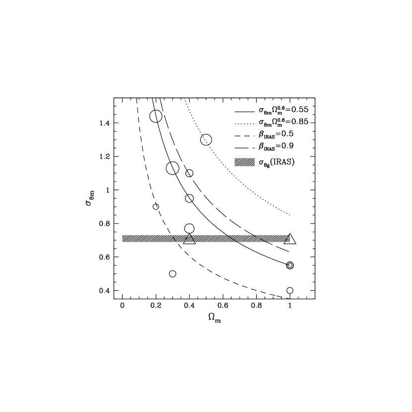
Figure 13: Points show the locations of the 15 models in the $\Omega_{m}-\sigma_{8m}$ plane, classified as Accepted (circles), or Rejected (triangles). The radius of the circles is proportional to $(10-\left<{\rm Rank}\right>)$, where $\left<{\rm Rank}\right>$ is the mean rank for the PSCz reconstruction of a model; larger circles represent more successful reconstructions. The lines show constraints in this plane derived from four different techniques: (1) $\sigma_{8m}\Omega_{m}^{0.6}=0.55$ from the abundance of clusters at $z=0$ (solid line), (2) $\sigma_{8m}\Omega_{m}^{0.6}=0.85$ from a maximum likelihood estimate of the mass power spectrum using peculiar velocity data (dotted line), (3) $\beta_{\rm IRAS}=0.5$ from the VELMOD analysis of the Mark III catalog of peculiar velocities and the IRAS 1.2 Jy galaxy redshift catalog (short dashed line), and (4) $\beta_{\rm IRAS}=0.9$ from the POTENT analysis of the Mark III catalog of peculiar velocities and the IRAS 1.2 Jy galaxy redshift catalog (long dashed line). The shaded region shows the observed fluctuation amplitude of the IRAS galaxy distribution, $\sigma_{8g}({\rm IRAS})=0.69\pm 0.04$.

Based on the ranks of the 15 models in Table 2, and their locations in Figure 13, we arrive at the following conclusions.

(1):

Our successful reconstructions of the PSCz catalog, at least for some plausible assumptions about the value of $\Omega_{m}$ and the bias between IRAS galaxies and mass, lends support to the hypothesis that LSS originated in the gravitational instability of small amplitude, Gaussian primordial mass density fluctuations. While this success does not, by itself, rule out non-Gaussian models for primordial fluctuations, it strengthens the viability of Gaussian models. Models whose initial conditions have substantially non-Gaussian PDFs generally predict quite different properties for LSS (Moscardini et al. (1991); Weinberg & Cole (1992)).

(2):

Unbiased models in which IRAS galaxies trace mass are rejected, for both $\Omega_{m}=0.4$ and $\Omega_{m}=1$. From Table 2 and the discussion in §5, it is clear that the models E1UNb1.0 and O4UNb1.0 are both clearly rejected by the reconstruction analysis of the PSCz catalog. Figure 11(a) shows that the model E1UNb1.0 fails in the manner expected if we reconstruct the redshift-space galaxy distribution in a low $\Omega_{m}$ universe using, erroneously, a high value of $\Omega_{m}$. The high velocity dispersion of clusters in an $\Omega_{m}=1$ model suppresses the small scale correlations in redshift space, while the large scale bulk flows, whose amplitude is proportional to $\Omega_{m}^{0.6}$, enhances the correlations on large scales. Therefore, the reconstructed $\xi(s)$ has a shallower slope compared to the true $\xi(s)$, although the rms fluctuations (in redshift space) of the two galaxy distributions are similar, by construction.

(3):

Of the five models with $\Omega_{m}=1$, E1THb1.3 is the only Accepted model that reconstructs the PSCz catalog as well as its own typical mock catalog. While the model E1UNb1.0 is clearly Rejected, the models E1PLb1.3 and E1PLb1.8 are Accepted because one mock catalog in each of these models is reconstructed worse than the PSCz catalog, and the model E1PLMDb1.3 is Accepted because there are two mock catalogs that are reconstructed worse than the PSCz catalog. Thus, although four of the five models with $\Omega_{m}=1$ are Accepted, most of them are only moderately successful in reconstructing the PSCz catalog.

(4):

In Figure 13, there are five models that lie on, or close to, the constraint $\beta_{\rm IRAS}=0.5$. Of these, the models O4UNb1.0 and O4SQEb1.0 are clearly rejected, the models E1Plb1.8 and L2PLb0.77 are Accepted because there is one mock catalog that is reconstructed worse than the PSCz catalog, while the model O3PLb1.4 is Accepted because there are two mock catalogs that are reconstructed worse than the PSCz catalog. All these models are at best only moderately successful in reconstructing the PSCz catalog. This leads us to conclude that the low-normalization constraint $\beta_{\rm IRAS}=0.5$ (corresponding to $\sigma_{8m}\Omega_{m}^{0.6}\approx 0.35$), inferred from the simplest interpretation of the VELMOD (Willick & Strauss (1998)) and redshift-space distortion (Cole et al. (1995)) analyses of the $1.2$Jy redshift survey, is only marginally successful in reconstructing the PSCz catalog. Here we have assumed that $b_{\delta}=b=\sigma_{8g}/\sigma_{8m}$ to convert an estimate of $\beta_{\rm IRAS}$ into a constraint on $\sigma_{8m}\Omega_{m}^{0.6}$. While this relation is valid in a deterministic, linear bias model, in the case of a more general biasing relation between galaxy and mass distributions, the relation between $b$ and $b_{\delta}$ also includes terms arising from the non-linearity and the stochasticity of the biasing relation (Dekel & Lahav (1999)). We are currently investigating the extent to which the estimates of $\beta_{\rm IRAS}$ using different techniques, including POTENT, VELMOD, and the anisotropy of the redshift-space power spectrum, are sensitive to the details of the biasing scheme (Berlind, Narayanan, & Weinberg, in preparation).

(5):

There are seven models including E1THb1.3, O2PLb0.5, O4MDb0.7, O4SAb0.9, L3PLb0.62, L4PLb0.64, and L5PLb0.54, in which the PSCz catalog is reconstructed better than at least three mock catalogs corresponding to that model. These models are the most successful in reconstructing the properties of the galaxy distribution in the PSCz catalog. Except for the model E1THb1.3, all these models have $\Omega_{m}<1$ and require that $\sigma_{8m}>\sigma_{8g}$ (hence $b<1$), i.e., that IRAS galaxies be antibiased with respect to the mass distribution on a scale of $8{h^{-1}\;{\rm Mpc}}$. However, we are unable to pin down the bias factor more precisely: the model O4SAb0.9, with a small antibias, and the model O2PLb0.5, with a large antibias, both reconstruct the PSCz catalog very well. Most of the successful models require that $\beta_{\rm IRAS}\geq 0.8$ (except the model O4SAb0.9, which requires $\beta_{\rm IRAS}\approx 0.7$)

(6):

The model O4SAb0.9, in which IRAS galaxies are related to the mass distribution according to the predictions of the semi-analytic galaxy formation model, reconstructs the PSCz catalog very well. This accurate reconstruction of the PSCz catalog is a non-trivial success of the semi-analytic model, since the models O4UNb1.0 and O4SQEb1.0, with quite similar values of $\Omega_{m}$ and $\sigma_{8m}$ but with different biasing relations, are both clearly rejected. This sensitivity of the reconstruction to the nature of the biasing relation demonstrates that the reconstruction analysis of a galaxy redshift survey can distinguish between different bias models, and not just between different values of the bias factor $b$.

Conclusions $(2)-(6)$ are based on reconstructing the PSCz catalog under the general assumptions that the primordial mass density fluctuations form a Gaussian random field and that the bias between IRAS galaxies and mass can be characterized by a local, monotonic function. While the assumption of Gaussian initial fluctuations enables us to constrain the nature of the biasing relation, we could also use reconstruction analysis in a complementary mode, i.e., to test the level of non-Gaussianity of the initial fluctuations, given our current state of knowledge of the galaxy formation process. In this regard, the successful reconstruction for a model (O4SAb0.9) based on a physically motivated theory of galaxy formation and cosmological parameter values supported by independent constraints supports the standard hypothesis that primordial fluctuations were not far from Gaussian.

There are several natural directions for extending this analysis using observational data. In this paper, we have compared the properties of the reconstruction to the input PSCz galaxy distribution in redshift space alone. However, every model reconstruction predicts both the real-space galaxy distribution and the fully non-linear peculiar velocity field at every point within the reconstruction volume. We can then compare the velocity field predicted for any model with the observed peculiar velocities of galaxies in, say, the Mark III catalog (Willick et al. 1997b ) or the SFI catalog (Giovanelli et al. (1997)). Such a comparison will be more accurate than a comparison involving the velocity field predicted using linear theory. The amplitude and the non-linear components of the velocity field serve as good diagnostics of the allowed values of $\Omega_{m}$ and $\sigma_{8m}$ (Narayanan & Weinberg (1998)). We can correct for inhomogeneous Malmquist bias when comparing the observed density and velocity fields by using the reconstructed line-of-sight density and velocity distributions to every galaxy. Alternatively, we can circumvent the effects of Malmquist bias by working directly in redshift space itself (Strauss & Willick (1995)).

In order to understand the galaxy formation process, it is necessary to study the relative bias between different types of galaxies as well as the absolute bias between the galaxy population as a whole and the underlying mass. For example, it is now well known that optical galaxies are more strongly clustered than IRAS galaxies (Lahav et al. (1990); Strauss et al. (1992); Saunders et al. (1992); Peacock & Dodds (1994); Willmer et al. (1998); Baker et al. (1998)). Reconstruction analysis of the galaxy distribution in the Optical Redshift Survey (Santiago et al. 1995, 1996), using a set of models similar to the ones discussed in this paper, will give us independent constraints on $\Omega_{m}$ and $\sigma_{8m}$ and enable us to test whether optical galaxies trace the underlying mass. Since the Optical Redshift Survey and PSCz probe similar regions of space, the initial conditions derived from reconstruction of the two data should be consistent with each other, and it should be possible to reproduce one catalog beginning with the initial conditions derived from the other by changing only the biasing model used to select galaxies from the evolved mass distribution.

Reconstruction analysis is thus a powerful tool to constrain the ranges of allowed values of cosmological parameters and the details of the galaxy formation process. For example, we can discriminate between models with low and high values of $\Omega_{m}$, and between models with different values of $\sigma_{8m}$ (hence, different values of $b$). However, if the cosmological parameters and the mass power spectrum can be determined precisely using other constraints, such as Type Ia supernovae, cosmic microwave background anisotropies, the Lyman-$\alpha$ forest, or weak lensing, then reconstruction analysis can focus on deriving the biasing relation between the different galaxy distributions and the underlying mass distribution. Knowledge of these relations will, in turn, provide strong tests of numerical and semi-analytic models for galaxy formation.

References

- Abell (1958) Abell, G. O. 1958, ApJS, 50, 241
- Babul & Postman (1990) Babul, A., & Postman, M. 1990, ApJ, 359, 280
- Bagla & Padmanabhan (1997) Bagla, J.S., & Padmanabhan, T. 1997, MNRAS, 286, 1023
- Baker et al. (1998) Baker, J.E., Davis, M., Strauss, M.A., Lahav, O., & Santiago, B.X 1998, ApJ, 508, 6
- Balian & Schaeffer (1989) Balian, R., & Schaeffer, R. A&A, 220, 1
- Bardeen et al. (1983) Bardeen, J.M., Steinhardt, P.J., & Turner, M.S. 1983, Phys Rev D, 28, 679
- Beacom et al. (1991) Beacom, J.F., Dominik, K.G., Melott, A.L., Perkins, S.P., & Shandarin, S.F. 1991, ApJ, 372, 351
- Benson et al. (1999) Benson, A.J., Cole, S., Frenk, C.S., Baugh, C.M., & Lacey, C.G 1999, MNRAS, submitted, (astro-ph/9903343)
- Bertschinger (1987) Bertschinger, E., 1987, ApJ, 323, L103
- Branchini et al. (1999) Branchini, E., et al. 1999, MNRAS, in press
- Brown & Peebles (1987) Brown, M.E., & Peebles, P.J.E., 1987, ApJ, 317, 588
- Canavezes et al. (1998) Canavezes, A., et al. 1998, MNRAS, 297, 777
- Cen & Ostriker (1992) Cen, R., & Ostriker, J. P. 1992, ApJ, 399, L113
- Cen & Ostriker (1993) Cen, R., & Ostriker, J. P. 1993, ApJ, 417, 415
- Cole et al. (1994) Cole, S., Aragon-Salamanca, A., Frenk, C.S., Navarro, J.F., & Zepf, S.E. 1994, MNRAS, 271, 781
- Cole et al. (1995) Cole, S., Fisher, K.B., & Weinberg, D.H 1995, MNRAS, 275 515
- Cole et al. (1997) Cole, S., Weinberg, D. H., Frenk, C. S., & Ratra, B. 1997, MNRAS, 289, 37
- Cole et al. (1998) Cole, S., Hatton, S., Weinberg, D. H., & Frenk, C. S. 1998, MNRAS, 300, 945 (CHWF98)
- Cole et al. (1999) Cole, S., Lacey, C., Baugh, C. & Frenk, C.S. 1999, MNRASsubmitted
- Couchman, H.M.P. (1991) Couchman, H. M. P. 1991, ApJ, 368, L23
- Croft & Gaztañaga (1997) Croft, R.A.C., & Gaztañaga, E. 1997, MNRAS, 285, 793
- Davis & Geller (1976) Davis, M., & Geller, M. J. 1976, ApJ, 208, 13
- Davis & Peebles (1983) Davis, M., & Peebles, P.J.E. 1983, ApJ, 267, 465
- Davis et al. (1996) Davis, M., Nusser, A., & Willick, J.A. 1996, ApJ, 473, 22
- Dekel & Lahav (1999) Dekel, A. & Lahav, O. 1999, ApJ, 520, 24
- de Lapparent, Geller & Huchra (1986) de Lapparent, V., Geller, M.J. & Huchra, J.P. 1986, ApJ, L1
- Dressler (1980) Dressler, A. 1980, ApJ236, 351
- Efstathiou et al. (1992) Efstathiou, G., Bond, J.R. & White, S.D.M, 1992, MNRAS, 258, 1P
- Einasto et al. (1994) Einasto, J., Saar, E., Einasto, M., Freudling, W., & Gramann, M. 1994, ApJ, 429, 465
- Eke et al. (1996) Eke, V.R, Cole, S., & Frenk, C.S. 1996, MNRAS, 282, 263
- Fisher et al. (1994) Fisher, K.B., Davis, M., Strauss, M.A., Yahil, A., & Huchra, J. 1994, MNRAS, 266, 50
- Fisher et al. (1995) Fisher, K.B., Huchra, J., Davis, M., Strauss, M.A., Yahil, A., & Schlegel, D. 1995, ApJS, 100, 69
- Freudling et al. (1999) Freudling, W., et al. 1999, ApJ, ApJ, 523, 1
- Gaztañaga et al. (1995) Gaztañaga, E., Croft, R.A.C., & Dalton, G.B 1995, MNRAS276, 336
- Gaztañaga & Baugh (1998) Gaztañaga, E., & Baugh, C.M 1998, MNRAS, 294, 229
- Giovanelli, Haynes & Chincarini (1986) Giovanelli, R., Haynes, M. P., & Chincarini, G. L. 1986, ApJ, 300, 77
- Giovanelli & Haynes (1989) Giovanelli, R., & Haynes, M.P., 1989, AJ, 97, 3
- Giovanelli et al. (1997) Giovanelli, R., Haynes, M.P., Herter, T., Vogt, N.P., Wegner, G., Salzer, J.J., da Costa, L.N., & Freudling, W. 1997, AJ, 113, 22
- Giraud (1986) Giraud, E. 1986, A&A, 170, 1
- (40) Gramann, M. 1993a, ApJ, 405, 449
- (41) Gramann, M. 1993b, ApJ, 405, L47
- Gramann et al. (1994) Gramann, M., Cen, R., & Gott, R.J. 1994, ApJ, 425, 382
- Guth & Pi (1982) Guth, A.H., & Pi, S.Y. 1982, Phys Rev Let, 49, 1110
- Guzzo et al. (1997) Guzzo, L., Strauss, M. A., Fisher, K. B., Giovanelli, R. & Haynes, M. P. 1997, ApJ, 489, 37
- Hamilton (1993) Hamilton, A.J.S. 1993, ApJ, 417, 19
- Hamilton (1998) Hamilton, A.J.S. 1998, in The Evolving Universe, ed. D. Hamilton, Kluwer Academic, p. 185
- Hawking (1982) Hawking, S.W. 1982, Physics Letters, 115, 295
- Hermit et al. (1996) Hermit, S., Santiago, B.X., Lahav, O., Strauss, M.A., Davis, M., Dressler, A. & Huchra, J. 1996, MNRAS, 283, 709
- Hockney & Eastwood (1981) Hockney, R. W., & Eastwood, J. W. 1981, Computer Simulations Using Particles, (New York: McGraw Hill)
- Hoffman & Ribak (1991) Hoffman, Y. & Ribak, E., 1991, ApJ, 380, L5
- Hubble (1936) Hubble, E.P. 1936, The Realm of the Nebulae (Oxford University Press: Oxford), 79
- Huchra & Geller (1982) Huchra, J. P., & Geller, M. J. 1982, ApJ, 257, 423
- Hudson (1993) Hudson, M.J. 1993, MNRAS, 265, 43
- Jenkins et al. (1998) Jenkins, A., et al. 1998, ApJ, 499, 20
- Kaiser (1987) Kaiser, N. 1987, MNRAS, 227, 1
- Kolatt et al. (1996) Kolatt, T., Dekel, A., Ganon, G., & Willick, J.A. 1996, ApJ, 458, 419
- Lahav et al. (1990) Lahav, O., Nemiroff, R.J., & Piran, Y. 1990, ApJ, 350, 119
- Lahav & Saslaw (1992) Lahav. O., & Saslaw, W.C. 1992, ApJ, 396, 430
- Lawrence et al. (1986) Lawrence, A., Walker, D., Rowan-Robinson, M., Leech, K.J., & Penston, M.V. 1986, MNRAS, 219, 687
- Little et al. (1991) Little, B., Weinberg, D.H, & Park, C. 1991, MNRAS, 253, 295
- Little & Weinberg (1994) Little, B., & Weinberg, D.H. 1994, MNRAS, 267, 605
- Loveday et al. (1995) Loveday, J., Maddox, S. J., Efstathiou, G., & Peterson, B. A. 1995, ApJ, 468, 442
- Lynden-Bell et al. (1989) Lynden-Bell, D., Lahav, O., & Burstein, D. 1989, MNRAS, 241, 325
- Maddox et al. (1990) Maddox, S.J.M., Efstathiou, G., Sutherland, W.J, & Loveday, J. 1990, MNRAS, 242,43
- Maddox et al. (1996) Maddox, S.J.M., Efstathiou, G., & Sutherland, W.J 1996, MNRAS, 283, 1227
- Meiksin & Davis (1986) Meiksin, A., & Davis, M. 1986, AJ, 91, 191
- Melott & Shandarin (1990) Melott, A.L., & Shandarin, S.F 1990, Nature, 346, 633
- Melott & Fry (1986) Melott, A.L., & Fry, J.N. 1986, ApJ, 305, 1
- Melott & Dominik (1993) Melott, A.L., & Dominik, K.G. 1993, ApJS, 86, 1
- Moore et al. (1994) Moore, B., Frenk, C.S., Efstathiou, G., & Saunders, W. 1994, MNRAS, 269, 742
- Moore et al. (1993) Moore, B., Frenk, C.S., & White, S.D.M. 1993, MNRAS, 261, 827
- Moscardini et al. (1991) Moscardini, L., Matarrese, S., Lucchin, F. & Messina, A. 1991, MNRAS, 248, 424
- Narayanan & Weinberg (1998) Narayanan, V.K, & Weinberg, D.H 1998, ApJ, 508, 440 (NW98)
- Narayanan & Croft (1999) Narayanan, V.K, & Croft, R.A.C. 1999, ApJ, 515, 471
- Nolthenius & White (1987) Nolthenius, R., & White, S.D.M 1987, MNRAS, 235, 505
- Nusser & Dekel (1992) Nusser, A., & Dekel, A. 1992, ApJ, 391, 443
- Nusser, Dekel, & Yahil (1995) Nusser, A., Dekel, A., & Yahil, A. 1995, ApJ, 449, 439
- Park, C. (1990) Park, C. 1990, PhD Thesis, Princeton University.
- Peacock & Dodds (1994) Peacock, J.A., & Dodds, S.J. 1994, MNRAS, 267, 1020
- Peebles (1980) Peebles, P.J.E. 1980, The Large Scale Structure of the Universe, (Princeton: Princeton Univ. Press)
- Postman & Geller (1984) Postman, M., & Geller, M.J. 1984, ApJ, 281, 95 (PG84)
- Ryden & Gramann (1991) Ryden, B., & Gramann, M. 1991, ApJ, 383, L33
- Sandage (1986) Sandage, A. 1986, ApJ, 301, 1
- Sandage & Tammann (1975) Sandage, A., & Tammann, G.A. 1975, ApJ, 196, 313
- Santiago et al. (1995) Santiago, B.X., Strauss, M.A., Lahav, O., Davis, M., Dressler, A., &
- Santiago et al. (1996) Santiago, B.X., Strauss, M.A., Lahav, O., Davis, M., Dressler, A., &
- Sargent & Turner (1977) Sargent, W. W., & Turner, E. L. 1977, ApJ, 212, L3
- Saunders et al. (1992) Saunders W., Rowan-Robinson, M., & Lawrence, A. 1992, MNRAS258, 134
- Saunders et al. (1995) Saunders W., Sutherland, W., Efstathiou, G., & Tadros, H. 1995, in Wide Field Spectroscopy and the Distant Universe, eds. S.J.Maddox & Aragón-Salamanca, A., (Singapore: World Scientific), p. 88
- Schlegel et al. (1994) Schlegel, D., Davis, M., Summers, F. & Holtzman, J.A 1994, 427, 527
- Sheth (1996) Sheth, R.K. MNRAS, 1996, 278, 101
- Sigad et al. (1998) Sigad, Y., Eldar, A., Dekel, A., Strauss, M. A., & Yahil, A. 1998, ApJ, 495, 516S
- Smoot et al. (1991) Smoot, G.F et al. 1991, ApJ, 371, L1
- Smoot et al. (1992) Smoot, G.F et al. 1992, ApJ, 396, L1
- Soda & Suto (1992) Soda, J., & Suto, Y. 1992, ApJ, 396, 379
- Soifer et al. (1984) Soifer, B.T. et al. 1984, ApJ, 278, L71
- Springel & White (1998) Springel, V., White, S.D.M. 1998, MNRAS, 298, 143
- Starobinsky (1982) Starobinsky, A. A. 1982, Phys Lett B, 117, 175
- Strauss et al. (1992) Strauss, M.A., Davis, M., Yahil, A., & Huchra, J.P. 1992, ApJ, 385, 421
- Strauss & Willick (1995) Strauss, M.A. & Willick, J.A., 1995, Physics Reports, 261, 271
- Tadros et al. (1998) Tadros, H., Efstathiou, G., & Dalton, G.B 1998, MNRAS, 296, 995
- van de Weygaert & Bertschinger (1996) van de Weygaert, R., & Bertschinger, E., 1996, MNRAS, 281, 84V
- Viana & Liddle (1996) Viana, P.T.P, & Liddle, A.R. 1996, MNRAS, 281, 323
- Vogeley et al. (1992) Vogeley, M.S., Park, C., Geller, M.J., & Huchra, J.P 1992, ApJ, 391, L5
- Weinberg (1989) Weinberg, D.H. 1989, PhD Thesis, Princeton University.
- Weinberg (1992) Weinberg, D.H. 1992, MNRAS, 254, 315
- Weinberg & Cole (1992) Weinberg, D.H., & Cole, S. 1992, MNRAS, 259, 652
- Weinberg, Gott & Melott (1987) Weinberg, D.H., Gott, R.J., & Melott, A.L., 1987, ApJ, 321, 2
- White (1979) White, S.D.M. 1979, MNRAS, 186, 145
- White et al. (1993) White, S.D.M., Efstathiou, G., & Frenk, C.S. 1993, MNRAS, 262, 1023
- Whitmore, Gilmore, & Jones (1993) Whitmore, B. C., Gilmore, D. M., & Jones, C. 1993, ApJ, 407, 489
- (112) Willick, J.A., Strauss, M.A., Dekel, A., & Kolatt, T. 1997a, ApJ, 486, 629
- (113) Willick, J.A., Courteau, S., Faber, S.M., Burstein, D., Dekel, A., & Strauss, M.A. 1997b, ApJS, 109, 333
- Willick & Strauss (1998) Willick, J. A., & Strauss, M. A. 1998, ApJ, 507, 64
- Willmer et al. (1998) Willmer, C. N. A., da Costa, L. N., & Pellegrini, P. S. 1998, AJ, 115, 869
- Yahil et al. (1991) Yahil, A., Strauss, M.A., Davis, M. & Huchra, J.P., 1991, ApJ, 372, 380
- Zel’dovich (1970) Zel’dovich, Ya. B. 1970 A&A, 5, 84
- Zwicky (1937) Zwicky, F. 1937, ApJ, 86, 217