Topology and geometry of the CfA2 redshift survey

Abstract

We analyse the redshift space topology and geometry of the nearby Universe by computing the Minkowski functionals of the Updated Zwicky Catalogue (UZC). The UZC contains the redshifts of almost 20,000 galaxies, is 96% complete to the limiting magnitude $m_{\rm Zw}=15.5$ and includes the Center for Astrophysics (CfA) Redshift Survey (CfA2). From the UZC we can extract volume limited samples reaching a depth of 70$h^{-1}{\rm Mpc}$ before sparse sampling dominates. We quantify the shape of the large–scale galaxy distribution by deriving measures of planarity and filamentarity from the Minkowski functionals. The nearby Universe shows a large degree of planarity and a small degree of filamentarity. This quantifies the sheet–like structure of the Great Wall which dominates the northern region (CfA2N) of the UZC. We compare these results with redshift space mock catalogues constructed from high resolution $N$–body simulations of two Cold Dark Matter models with either a decaying massive neutrino ($\tau$CDM) or a non–zero cosmological constant ($\Lambda$CDM). We use semi–analytic modelling to form and evolve galaxies in these dark matter–only simulations. We are thus able, for the first time, to compile redshift space mock catalogues which contain galaxies, along with their observable properties, rather than dark matter particles alone. In both models the large scale galaxy distribution is less coherent than the observed distribution, especially with regard to the large degree of planarity of the real survey. However, given the small volume of the region studied, this disagreement can still be a result of cosmic variance, as shown by the agreement between the $\Lambda$CDM model and the southern region of CfA2.

1 Introduction

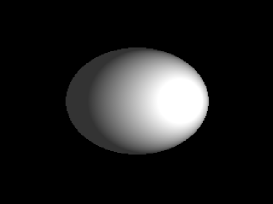
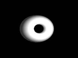
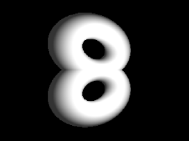
Figure 1: Simple structures with positive (egg, left panel), vanishing (loop, middle panel), and negative (double loop, right panel) Euler characteristic $V_{3}$.

Standard inflationary models (e.g. peacock:cosmological) predict that the large–scale structure of the present day Universe originates from primordial density perturbations amplified by gravitational instability. Under the influence of its own gravity, the initial Gaussian random field of the density fluctuations evolves into a strongly non–Gaussian density field. Therefore, in order to describe the observed galaxy distribution quantitatively, we need statistics beyond the traditional Fourier transform pair $P(k)$ and $\xi(r)$, the power spectrum and the two–point correlation function. In fact, these quantities only describe a Gaussian density field in a unique and complete way.

One possible approach to capturing higher–order features of the galaxy distribution involves geometrical descriptors. A number of these statistics have been suggested to date. Among others, recent morphological analyses of the nearby Universe have been performed through measuring the void probability function of the CfA2 catalogue [Vogeley et al.1994a], applying percolation techniques to the IRAS 1.2Jy catalogue [Yess et al.1997] and the Las Campanas Redshift Survey (LCRS) [Shandarin & Yess1998], or through various types of shape statistics, as the moment–of–inertia method suggested by babul:filament and applied by dave:filament to the CfA1 redshift survey and by sathyaprakash:filaments to the IRAS 1.2Jy catalogue. The most wide–spread technique is probably the genus statistics introduced by gott:sponge, which has been used on various IRAS catalogues [Moore et al.1992, Protogeros & Weinberg1997, Canavezes et al.1998, Springel et al.1998], on the CfA2 redshift survey [Vogeley et al.1994b] and, in a modified way, on the nearly two–dimensional LCRS [Colley1997]. With galaxy clusters, scales of several hundred $h^{-1}{\rm Mpc}$ have been probed using different morphological statistics [Coles et al.1998, Plionis et al.1992], including the Minkowski functionals [Kerscher et al.1997].

Among this plethora of methods, Minkowski functionals currently represent the most comprehensive description of the topological and geometric properties of a three–dimensional structure. Minkowski functionals include both the percolation analysis and the genus curve. Minkowski functionals can be applied both to density fields [Schmalzing & Buchert1997] and to discrete point sets [Mecke et al.1994], where the latter approach has the advantage of introducing just one single diagnostic parameter (see below for details), rather than, for example, a smoothing length and a threshold as in the genus statistics. Because Minkowski functionals are additive they are robust measures even for sparse samples. Minkowski functionals also discriminate different cosmological models efficiently [Schmalzing et al.1999a]. Finally, Minkowski functionals can be used to define a planarity ${\mathcal{P}}$ and a filamentarity ${\mathcal{F}}$ and thus quantify our intuition about the shape of a structure [Sahni et al.1998].

Here, we study the redshift space topology of the nearby Universe by analysing the Updated Zwicky Catalogue (UZC, falco:uzc) which contains the redshifts of almost 20,000 galaxies and is 96% complete in more than one fifth of the sky to the limiting Zwicky magnitude $m_{\text{Zw}}=15.5$. The UZC includes the CfA2 Redshift Survey [Huchra et al.1999, Huchra et al.1995, Huchra et al.1990, Geller & Huchra1989, Huchra et al.1983, de Lapparent et al.1986, Davis et al.1982]. In our analysis, we use the Minkowski functionals and their associated shape quantifiers planarity ${\mathcal{P}}$ and filamentarity ${\mathcal{F}}$ which we define in Appendix B. Recently, a similar analysis on the nearby Universe has been performed by using the LCRS [Bharadwaj et al.1999]. The main advantage of using the UZC over the LCRS is the geometry of the survey: the LCRS consists of six separated slices only 1$\aas@@fstack{\circ}$5 thick; thus, an analysis of the full three–dimensional structure cannot be performed. In fact, bharadwaj:evidence are unable to discriminate whether the “filaments” seen in the LCRS are actually sections of “sheets”. Because the UZC consists of two coherent regions covering $\sim 14$% and $\sim 7$% of the sky respectively without discontinuities, we can address this point here. In fact, geller:mapping were the first to address the two–dimensionality of the structures by identifying the “Great Wall” in the CfA2 redshift survey. On the other hand, with the UZC, we can only probe the topology of a volume 70$h^{-1}{\rm Mpc}$ deep, which is too small to be representative of the Universe.

We compare the UZC redshift space topology with mock galaxy redshift surveys extracted from $N$–body simulations of a Cold Dark Matter (CDM) model including galaxies modelled with semi–analytical techniques [Kauffmann et al.1999a]. Therefore the density bias, the distribution of galaxies relative to the dark matter, is taken self–consistently into account by including the physics of galaxy formation and evolution explicitly.

In Section 2 we review our analysis method. Section 3 briefly describes the properties of the UZC catalogue and presents the results of our topological analysis. We compare the northern region of the CfA2 redshift survey with the mock catalogues in Section 4. We summarise in Section 5. Two appendices provide important but gory details of Minkowski functional analysis.

2 Method

2.1 Minkowski functionals

	geometric quantity	$\mu$	$V_{\mu}$
$V$	volume	0	$V$
$A$	surface	1	$A/6$
$H$	mean curvature	2	$H/3\pi$
$\chi$	Euler characteristic	3	$\chi$

Table 1: Minkowski functionals $V_{\mu}$ expressed in terms of the corresponding geometric quantities.

Figure 2: Surface area and the integrated mean curvature, namely the Minkowski functionals $V_{1}$ and $V_{2}$, for spheroids of varying axis ratio. Prolate spheroids (“cigars”) are characterised by large surface area and comparatively small mean curvature, while the situation is reversed for oblate spheroids (“pancakes”).

Minkowski functionals are named after minkowski:volumen, in acknowledgment of his pioneering contributions to integral geometry (for an up–to–date overview of the theory see, for example, schneider:brunn). mecke:robust introduced the Minkowski functionals into cosmology as descriptors of the geometry and topology of a distribution of points. One appealing property of the Minkowski functionals is their uniqueness and completeness as morphological measures, which follows by the theorem of hadwiger:vorlesung on very general requirements. Furthermore, the four Minkowski functionals in three dimensions can be interpreted as well–known geometric quantities, as summarised in Table 1.

Figure 1 shows examples of bodies with different Euler characteristic $V_{3}$. The Euler characteristic is a purely topological quantity and measures the connectivity of a set. It is equal to the number of parts minus the number of holes. Hence the egg (left panel) has $V_{3}=1$, while the single (middle panel) and double loop (right panel) have $V_{3}=0$ and $V_{3}=-1$, respectively. The behaviour of the surface area $V_{1}$ and mean curvature $V_{2}$ is illustrated in Figure 2 on a simple family of spheroids, whose Minkowski functionals are known analytically [Hadwiger1955]. By varying the axis ratio of the spheroids while keeping the volume fixed, we obtain a curve in the $V_{1}$–$V_{2}$–plane. Values are given in units of the corresponding functionals of a sphere of the same volume, so we are indeed showing the effects of shape. A sphere would lie at the cusp at $(1,1)$. Prolate spheroids (“cigars”) are characterised by large surface area and comparatively small mean curvature, while the situation is reversed for oblate spheroids (“pancakes”).

We consider a volume–limited subsample from a galaxy catalogue as a set of points $\{{\bf x}_{i}\}$, where $i=1\ldots{N}$. Since the geometry of single points is trivial, we decorate each point with a ball $B$ of radius $r$, and measure the Minkowski functionals of the resulting union set, the so–called Boolean grain model [Wicksell1925]. In short, we construct the union set

$$A_{r}=\bigcup_{i=1}^{N}B_{{\bf x}_{i}}$$ (1)

and look upon the quantities $V_{\mu}\left(A_{r}\right)$ as functions of the ball radius $r$. By increasing the size of the balls, connections are established between points farther apart, until the survey volume is completely filled by the Boolean grain model. The radius can therefore be used as a diagnostic parameter.

2.2 Incomplete sky coverage and finite survey depth

Figure 3: The volume fraction of the reduced window as a function of the shrinking distance. The dashed line corresponds to full sky coverage of $4\pi$; the solid line is for the CfA2n window.

Currently, estimation of geometrical quantities such as Minkowski functionals relies on homogeneous sampling of the underlying point distribution. Galaxy catalogues, however, are usually magnitude–limited, and therefore intrinsically inhomogeneous. The standard solution is to use a series of volume–limited subsamples. However, even with volume–limited subsamples, care needs to be taken to obtain meaningful results that are not affected by the sample geometry. We summarise our approach here. An extensive description can be found in Appendix A.

For calculating the volume functional $v_{0}$, we use the unbiased estimator

$$v_{0}=\frac{V_{0}(A_{r}\cap{D}_{r})}{V_{0}(D_{r})},$$ (2)

where $D_{r}$ denotes the part of the volume, or window, $D$ that is farther than $r$ from the boundary. For all other Minkowski functionals, we use minus estimators constructed from partial Minkowski functionals. An unbiased estimator of the volume densities $v_{\mu}$ of the Minkowski functionals is obtained through

$$v_{\mu}=\frac{1}{|D_{2r}|}\sum_{i=1}^{N}\chi_{D_{2r}}({\bf x}_{i})V_{\mu}(A_{r};{\bf x}_{i})\qquad(\mu=1,2,3),$$ (3)

where $D_{2r}$ denotes the reduced sample window, and $\chi_{D_{2r}}$ is its characteristic function.

This approach works for arbitrary sky coverage, including the non–convex boundaries of the CfA2 survey. Moreover, at any radius, we use all available points, since points outside the reduced sample window still contribute as neighbours of points remaining inside. The only drawback of our approach, when compared to the method of schmalzing:minkowski, is that the window now shrinks by twice the radius. This fact considerably reduces the maximum allowed size of the Boolean ball.

We may quantify the loss of accuracy by the ratio $|D_{r}|/|D|$ between the volumes of the reduced and the original windows. For complete sky coverage, we have

$$\frac{|D_{r}|}{|D|}=\left(1-\frac{r}{R}\right)^{3}$$ (4)

where $R$ gives the depth of the volume–limited sample and $r$ is the distance to be kept from the boundary. If the sky coverage is not complete, this fraction decreases rapidly. This is illustrated in Figure 3, which compares the reduced window size for full sky coverage, and for the 10% sky coverage of the CfA2n window (defined in Section 4.1). Apparently, analysing the CfA2 catalogue with Minkowski functionals becomes impractical at radii above 10$h^{-1}{\rm Mpc}$. We set our maximum Boolean ball radius at 5$h^{-1}{\rm Mpc}$, so our results are not affected by this problem.

3 The Updated Zwicky Catalogue

We now briefly describe the properties of the Updated Zwicky Catalogue (UZC, Section 3.1). In Section 3.2 we compute its Minkowski functionals with the method based on the Boolean grain model.

3.1 Description

Figure 4: Cone diagram of the volume–limited subsample of 70$h^{-1}{\rm Mpc}$ depth we analyse here from the UZC. The larger and smaller cones correspond to the northern and southern region, respectively. The large dot marks the location of our galaxy and alludes to adams:hitchhiker.

falco:uzc provide new measurements of the positions and redshifts of most galaxies in the Zwicky Catalogue, which has been the basis for the CfA1 and CfA2 redshift surveys (see falco:uzc and references therein). The UZC represents a homogeneous and well calibrated redshift catalogue of almost 20,000 galaxies. Furthermore, the catalogue is now publicly available.

The UZC covers the northern celestial hemisphere which is not obscured by the Galactic disk; the redshift catalogue is $\sim 96\%$ complete to a limiting Zwicky magnitude $m_{\text{Zw}}=15.5$.

The CfA2 redshift surveys have been compiled over many years and this name has indicated progressively larger areas of the sky, as the surveys were reaching completion. The UZC contains all of the CfA2 survey analysed in the literature to April 1999. Following falco:uzc, we refer to the area with right ascension ranges $8{{}^{\rm h}}\leq\alpha_{1950}\leq 17{{}^{\rm h}}$ and $20{{}^{\rm h}}\leq\alpha_{1950}\leq 4{{}^{\rm h}}$ and declination range $-2\aas@@fstack{\circ}5\leq\delta_{1950}\leq 50\degr$ as the CfA2 region. The first right ascension range defines the CfA2N region containing 12,082 galaxies with measured redshift. The regions between 3^hand 4^hand between 20^hand 22^hare sparsely populated in the catalogue largely because of galactic obscuration. Therefore we restrict the CfA2S region to the 4,436 galaxy redshifts in the right ascension range $22{{}^{\rm h}}\leq\alpha_{1950}\leq 3{{}^{\rm h}}$. Both areas used in our analysis are more than 98% complete. Moreover the UZC contains some galaxies fainter than the magnitude limit. These galaxies are mainly in multiplets which were unresolved by Zwicky. They affect the properties of the galaxy distribution on very small scales but should leave our analysis unchanged. Note that the actual number of available redshifts in the UZC is currently increasing, as the catalogue is being updated.

Visual inspection shows well–defined structure in the CfA2 surveys, with large voids and sheet–like structures. Figure 4 shows a cone diagram of the volume–limited samples from CfA2N and CfA2S we analyse here. The dense feature close to the boundary of the northern part of the catalogue is the “Great Wall” (geller:mapping, see also Figure 6 of falco:uzc). In CfA2S, the apparent galaxy concentration is the Perseus–Pisces supercluster.

3.2 Topology and geometry

Figure 5: Minkowski functionals of CfA2N (solid line) and CfA2S (dashed line). All curves were calculated from volume–limited samples 70$h^{-1}{\rm Mpc}$ deep. Note that the CfA2N Minkowski functionals are systematically larger than the CfA2S ones, indicating larger clustering [Marzke et al.1995].

In our analysis, we use volume–limited samples 70$h^{-1}{\rm Mpc}$ deep. This provides a good compromise between object number (of all volume–limited subsamples, the 70$h^{-1}{\rm Mpc}$ one includes the highest number of objects) and depth (parts of the Great Wall are closer than 70$h^{-1}{\rm Mpc}$). Since the scaling behaviour of Minkowski functionals with the number density is not known in general, we take care to always analyse samples with the same number density of galaxies. From all volume–limited samples, we choose a set of slightly smaller random samples such that the number density corresponds to exactly 1,000 galaxies in the CfA2n volume (see Section 4.1 for a definition).

The results of our analysis of the UZC are shown in Figure 5. Instead of the Minkowski functionals $v_{\mu}$ themselves, we plot the quantities $1-{\overline{V}}_{\mu}/V_{\mu}(B)$. A thorough motivation of their use is given in Appendix B; most notably they are exactly equal to zero for a stationary Poisson process, i.e. a random distribution of points with spatially constant density. Generally speaking, values above zero reveal a clustered distribution of galaxies. Note, however, that the ${\overline{V}}_{\mu}$ can be written as an alternating series containing the hierarchy of correlation functions [Schmalzing et al.1999b], so clustering does not simply mean that the two–point function is positive. As an example, consider $1-{\overline{V}}_{0}/V_{0}(B)$. By Equation (13) this quantity increases monotonically with $1-v_{0}$, the void probability function [White1979]. Hence larger values in our plots indicate larger voids in the point distribution, which in turn means that points have to cluster more tightly.

Some of the functionals, most notably the volume $v_{0}$, indicate stronger clustering for CfA2N than for CfA2S. In fact, CfA2N contains more clusters than CfA2S and the Great Wall is more apparent than the Perseus–Pisces supercluster in CfA2S. The two–point correlation function already showed that the CfA2N clustering is peculiarly large when compared to other surveys [Marzke et al.1995, Diaferio et al.1999a].

We use a toy model to characterise the geometry of CfA2: we assume that galaxies are distributed in one–dimensional filaments, two–dimensional sheets or in a homogeneous field. We can compute the Minkowski functionals for this model analytically. Two coefficients, ${\mathcal{F}}$ and ${\mathcal{P}}$, give the relative contribution of filaments and sheets in the galaxy distribution (see Appendix B for details). Note, however, that this approach has the main shortcoming of assigning structures which are loosely clustered to the planarity component, because alternative assignments would yield considerably worse fits. Therefore, ${\mathcal{F}}$ and ${\mathcal{P}}$ yield the relative importance of the two structural components, but their exact values should be considered cautiously.

By fitting our toy model to the CfA2N Minkowski functional curves, we obtain ${\mathcal{F}}=0.12$ and ${\mathcal{P}}=0.67$ for the filamentarity and planarity contribution, respectively. The high degree of planarity is expected from the visual appearance of the Great Wall in the catalogue. For the CfA2S we find ${\mathcal{F}}=0.01$ and ${\mathcal{P}}=0.75$. The large value of ${\mathcal{P}}$ in both regions reflects the tendency of galaxies to be distributed in two–dimensional structures or in loose structures rather than in filaments. Moreover, the smaller size of the CfA2S region also tends to increase slightly the signal for planar and loose structures.

Because of its simplicity, our toy model provides a straightforward way of measuring planarity and filamentarity, but it is inadequate to model more complex realistic situations. We are planning some refinements in order to obtain results in better agreement with our intuitive interpretations of the galaxy distribution.

4 Mock galaxy redshift surveys

Figure 6: Cone diagrams of two mock catalogues. The upper and lower cones are a volume–limited subsample constructed from the CfALF $\Lambda$CDM model and the CfALF $\tau$CDM model, respectively. The observer galaxy is indicated by the large dot.

We compare the morphology of the CfA2n redshift survey with two variants of a CDM model. In Section 4.1 we briefly describe the simulations and how we model galaxy formation and evolution. Section 4.2 discusses how the luminosity limit of the galaxy sample, the shape of the sample volume and the peculiar velocity distortions in redshift space affect the Minkowski functionals. Section 4.3 contains the comparison of CfA2n with the mock galaxy redshift surveys.

4.1 Models

We consider two simulations from the GIF project [Kauffmann et al.1999a]: a CDM model with either $\Omega_{0}=1$ ($\tau$CDM) or $\Omega_{0}=0.3$ and $\Lambda=0.7$ ($\Lambda$CDM). The simulations contain $256^{3}$ dark matter particles each. The normalisation $\sigma_{8}$ of the power spectrum of the initial density perturbations was chosen to reproduce the present day abundance of rich galaxy clusters. Table 2 summarises the parameters of the models.

Table 2: GIF Simulations

model	$\Omega_{0}$	$\Omega_{\Lambda}$	$h$	$\sigma_{8}$	$m_{p}$	$L$
$\Lambda$CDM	0.3	0.7	0.7	0.90	1.4	141
$\tau$CDM	1.0	0.0	0.5	0.60	1.0	85

Parameters of the two GIF simulations [Kauffmann et al.1999a] used in this paper. The Hubble constant $h$, the particle mass $m_{p}$, and the comoving size $L$ of the simulation box are in units of $H_{0}=100{{\rm km}\,{\rm s}^{-1}}{\rm Mpc}^{-1}$, $10^{10}{h^{-1}M_{\odot}}$, and $h^{-1}{\rm Mpc}$, respectively.

The simulations were run with Hydra [Pearce & Couchman1997], the parallel version of the AP³M code [Couchman1991, Couchman et al.1995], kindly provided by jenkins:virgo.

kauffmann:clusteringI combine these high resolution $N$–body simulations with semi–analytic modelling to form and evolve galaxies within dark matter haloes: gas cooling, star formation, supernova feedback, stellar evolution and galaxy–galaxy merging are the relevant processes included. At any cosmological epoch, the observable properties of the galaxies, namely luminosity, colour, star formation rate, and stellar mass, are the result of the galaxy’s merging history, its interaction with the environment and the passive evolution of its stellar content.

The models predict photometric and clustering properties of galaxies at redshift $z=0$ [Kauffmann et al.1999a, Diaferio et al.1999a], and their evolution to high redshift [Kauffmann et al.1999b, Diaferio et al.1999b] which are in reasonable agreement with observations. Moreover, these analyses suggest further diagnostics for constraining the cosmological model and determining the relevance of the different galaxy formation processes.

These simulations represent the only models, available to date, where galaxies form and evolve in a self–consistent cosmological model and within a volume of the Universe sufficiently large for an analysis of the large scale galaxy distribution (see also pearce:simulation). In fact, diaferio:clusteringIII extract mock galaxy redshift surveys from the simulations at $z=0$ for a direct comparison with the CfA2N redshift survey, whose volume $\sim 7\times 10^{5}h^{-3}$Mpc³ is comparable to the volume of the simulation boxes. Specifically, they consider the area $8{{}^{\rm h}}\leq\alpha_{1950}\leq 17{{}^{\rm h}}$, $8\aas@@fstack{\circ}5\leq\delta_{1950}\leq 44\aas@@fstack{\circ}5$ which has a declination range smaller than CfA2N. We refer to this region as the CfA2n region. In order to resemble the CfA2n appearance in the mock catalogues as closely as possible, the mock redshift surveys were compiled by locating the observer home galaxy within the simulation box on a galaxy similar to the Milky Way at $\sim 70{h^{-1}{\rm Mpc}}$ away from a Coma–like massive cluster.

diaferio:clusteringIII analyse both the CfA2n and the mock redshift surveys with the same standard observational techniques. They show that the small scale clustering properties of galaxies, namely galaxy group properties, redshift space correlation function and pairwise velocities, are reproduced by both models independently of $\Omega_{0}$. Despite this success, a visual inspection of the mock redshift surveys shows remarkable differences in the large scale distribution of galaxies. Both models fail to produce structures as coherent and as sharply defined as in the CfA2n survey, although $\Lambda$CDM catalogues seem to be in better qualitative agreement with the data (see their Figures 5–8). Two examples of volume–limited subsamples constructed from these models are shown in Figure 6.

The $B$–band galaxy luminosity function predicted by the semi–analytical models is not a good fit to the CfA survey luminosity function [Marzke et al.1994]. To investigate the effect of the luminosity function on the small–scale clustering properties, diaferio:clusteringIII assign new luminosities to the galaxies in order to reproduce the CfA luminosity function exactly, while preserving the galaxies’ luminosity rank. We thus have two sets of mock catalogues, where the galaxies have luminosities according to the semi–analytical model luminosity function (SALF) or the CfA luminosity function (CfALF). We have analysed both the SALF and CfALF mock catalogues. Similarly to other measures related to the underlying mass distribution, the Minkowski functionals are basically independent of the luminosity function adopted. Throughout this analysis, we show results from the CfALF catalogues alone. Moreover, we consider ten mock catalogues for each simulation to assess the robustness of our results.

4.2 Luminosity, geometry and redshift space effect

Figure 7: Effect of luminosity and geometry on the Minkowski functionals of the CfALF $\Lambda$CDM model. The dashed and solid lines are for all galaxies in the simulation box brighter than $M_{\text{B}}=-18.7+5\log h$ and $M_{\text{B}}=-17.5+5\log h$ respectively. The shaded area indicates the $1\sigma$–spread over ten subsamples.

kauffmann:clusteringI show that the two–point correlation function is similar for galaxy samples with different magnitude limits. The Minkowski functionals are able to extract more information from the galaxy distribution. In fact, bright galaxies cluster stronger than faint ones. Figure 7 shows the Minkowski functionals for the $\Lambda$CDM simulation; $\tau$CDM yields very similar plots. In order to keep constant the statistical significance of different galaxy samples, we compute the Minkowski functionals only of subsamples containing the same number density of galaxies, and average over ten subsamples. The solid lines show the Minkowski functionals for galaxies brighter than $M_{B}=-17.5+5\log{h}$. The Minkowski functionals for galaxies brighter than $M_{B}=-18.7+5\log{h}$ are indicated by dashed lines. This absolute magnitude corresponds to an apparent magnitude $m_{B}=15.5$ at 70$h^{-1}{\rm Mpc}$. The difference between the two curves is significantly larger than the scatter between different subsamples from the same set of galaxies.

We have also checked that the Minkowski functionals computed with our procedure (Section 2.2) are insensitive to the shape of the sample volume. We do this by calculating the Minkowski functionals of the real space position of the galaxies averaged over the volume–limited subsamples extracted from the ten mock redshift surveys. The dashed lines in Figure 7 lie within the scatter of the resulting Minkowski functionals (shown as the dark shaded area in Figure 8). Since they come from volumes which have differing shape (periodic, rectangular box versus CfA2n volume ) but contain galaxies with roughly the same luminosity, we can deduce that the difference due to the sample geometry is negligible in comparison to the scatter between individual mock catalogues. Note that for mock catalogues, the scatter is much larger than for subsamples from the whole simulation box, simply because a mock catalogue contains fewer galaxies.

Figure 8: Minkowski functionals of the $\Lambda$CDM mock catalogues in real space (dark shaded area) and in redshift space (light shaded area). The shaded area indicates the r.m.s. spread over the ten mock catalogues.

Redshift space distortions tend to destroy structure on small scales, because groups and clusters in real space are diluted in redshift space by the finger–of–god effect. Figure 8 shows this difference in the $\Lambda$CDM model. The Minkowski functionals of the real and redshift space galaxy distributions almost coincide at larger values of the Boolean ball radius, because redshift space distortions become less relevant on large scale.

4.3 Comparison with the CfA2n

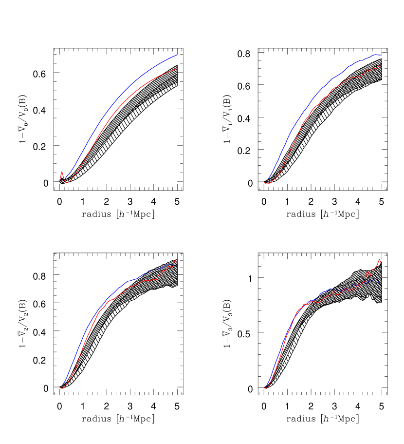
Figure 9: Structure in the CfA2n redshift survey, and in the mock catalogues extracted from the $\Lambda$CDM (dark shaded area) and the $\tau$CDM (light shaded area) models. The areas indicate the 1–$\sigma$ scatter over the ten mock catalogues constructed for each model. All curves are for volume–limited samples 70$h^{-1}{\rm Mpc}$ deep.

Figure 9 compares the morphological properties of CfA2n with the mock catalogues: neither of the two models is capable of reproducing the CfA2n properties. At Boolean ball radii $\sim 1-2{h^{-1}{\rm Mpc}}$, all the four Minkowski functionals of CfA2n are five times the r.m.s. above the average mock catalogue of the $\Lambda$CDM. Given the rather small number of ten realisations, we can conclude that the CfA2n clustering is not reproduced by the $\Lambda$CDM model at the 90% confidence level. The $\tau$CDM model shows an even smaller degree of clustering. At larger radii and for the mean curvature $v_{2}$ and Euler characteristic $v_{3}$, the disagreement between the models and observations is less dramatic, but also less significant, because the sample volume is filled by a considerably smaller number of Boolean balls. It is crucial to recall, however, that the scatter of quantities derived from the variance over all ten mock catalogues underestimates the sampling variance, because the mock surveys are constructed from the same small parent simulation.

The failure of the $\Lambda$CDM in reproducing the CfA2n Minkowski functionals is particularly interesting, because, on average, this model fits other observations reasonably well and in any case better than the $\tau$CDM model [Kauffmann et al.1999a, Kauffmann et al.1999b]. The Minkowski functionals confirm that $\Lambda$CDM should be preferred to $\tau$CDM.

It is worth noting that, because of the smaller degree of clustering of CfA2S when compared to CfA2N (see Figure 5), the difference between the CfA2S and the models is less pronounced, although still significant. The result is an example of the power of the Minkowski functionals analysis. In fact, diaferio:clusteringIII show that the two point correlation function of the mock catalogues agrees quite well with the CfA2S function. As expected, the Minkowski functionals are able to extract more information on the clustering properties of galaxies.

We can also perform the fitting procedure described in Appendix B to estimate the planarity and filamentarity of the structure contained in the mock catalogues. $\Lambda$CDM yields ${\mathcal{F}}=0.01$ and ${\mathcal{P}}=0.64$, while $\tau$CDM results in ${\mathcal{F}}=0.02$ and ${\mathcal{P}}=0.60$ for the average mock catalogues. As pointed out in Section 3.2, the large values of ${\mathcal{P}}$ compared to ${\mathcal{F}}$ indicate that the galaxies tend to be distributed in two–dimensional or loose structures rather than filaments. Compared to the values determined from the real CfA2N catalogue in Section 3.2 (${\mathcal{F}}=0.12$ and ${\mathcal{P}}=0.67$), ${\mathcal{P}}$ is $\sim 10\%$ smaller in the models than in CfA2N, again indicating a smaller degree of clustering.

We cannot exclude that the failure of the models in reproducing the Minkowski functionals of CfA2N is due to the small size of both the simulation box and the real survey. In fact, the initial power spectrum of the density perturbations does not contain Fourier components with wavelength larger than the box size. This prevents the development of large–scale non–Gaussian features such as the Great Wall. Moreover, as already indicated by an analysis of the IRAS 1.2Jy catalogue [Kerscher et al.1998], a volume–limited subsample 70$h^{-1}{\rm Mpc}$ deep is too small to be a fair sample of the Universe. Therefore, our analysis is likely to be dominated by local effects, which should average out when deeper catalogues are considered. This hypothesis could already be tested either with simulations of larger volumes (see e.g. doroshkevich:superlargescale), where one could estimate the cosmic variance, or with a constrained realisation [Mathis et al.1999], which should not suffer from the fair sample problem.

5 Conclusion

lapparent:slice and geller:mapping first pointed out that the large–scale galaxy distribution in the CfA2 redshift survey has a two–dimensional sheet–like structure rather than a one–dimensional filamentary appearance. Here we quantify this visual impression by analysing the redshift space topology and geometry of the UZC. By constructing a Boolean grain model of balls centred around the galaxies, we obtain unbiased estimates for the Minkowski functionals of the galaxy distribution. We then fit the Minkowski functionals to a toy model to extract quantitative information on the degree of filamentarity and planarity in CfA2. We find that filament– and sheet–like structures contribute 12% and 67% to the Minkowski functionals of CfA2N respectively, while the remainder comes from a homogeneous distribution of galaxies. Our results therefore strongly suggest that the filaments identified in the LCRS [Bharadwaj et al.1999] are actually sections of sheets.

Apparently, our simple model is inadequate in other realistic situations, such as CfA2S (the southern part of the UZC), where looser structures are present. However, the encouraging result we obtain with CfA2N indicates that it is worth pursuing this approach with some refinements. When deeper surveys as the Sloan Digital Sky Survey will be available, our approach can represent a valuable tool to quantify the topology of the galaxy distribution. Most notably, contrary to sahni:shapefinders or schmalzing:disentanglingI, the method presented here does not rely on shape measurements of isolated isodensity contours. Hence we can also obtain meaningful results in low to intermediate density environments, where objects in a smoothed field already percolate and are inaccessible to measurements.

We also compare CfA2n, a smaller volume of CfA2N, with mock redshift surveys extracted from a $\Lambda$CDM and a $\tau$CDM model. The models do not show the high degree of clustering of CfA2n. However, CfA2n seems to be quite a peculiar region of the Universe and the disagreement between the models and, for example, CfA2S is less dramatic. Moreover, the Minkowski functionals of the $\Lambda$CDM are closer to observations than the Minkowski functionals of $\tau$CDM. In conclusion, although our topological analysis confirms earlier results which indicate that overall $\Lambda$CDM is a better representation of the real Universe than $\tau$CDM, we show, at the same time, that $\Lambda$CDM is not yet a satisfactory model of the Universe.

vogeley:topology compare the genus statistics of CfA2 with a $\Lambda$CDM model. They find that this model is consistent with CfA2 on scales $\geq 10{h^{-1}{\rm Mpc}}$, but it fails to reproduce CfA2 on smaller scales. They use a simple bias scheme to identify galaxies and extract mock catalogues from $N$–body simulations. So the physics acting on small scales, which is missing from their simulations, might be responsible for the disagreement. Here, we used semi–analytic modelling to form and evolve galaxies in $N$–body simulations, but still the agreement between $\Lambda$CDM and CfA2 does not improve.

Note that our Boolean grain model approach follows a direction complementary to the genus statistics analysis generally used. The standard method introduced by gott:sponge employs a density field smoothed on varying scales. Increasing the smoothing kernel width successively erases structure on small scales [ter Haar Romeny et al.1991]. The analysis of vogeley:topology, for example, employs widths between 6$h^{-1}{\rm Mpc}$ and 20$h^{-1}{\rm Mpc}$ and addresses the issue of the Gaussianity of the distribution of the initial density perturbations. We adopt the Boolean grain model approach by mecke:robust and decorate each galaxy with a sphere of radius $r$ varying from zero to $5{h^{-1}{\rm Mpc}}$. This procedure captures the morphology of distinct structures on very large scales while preserving the small scale structure information.

Finally, the small volume of both the survey and our simulation boxes represents a severe limit to our analysis, because we are unable to quantify the effect of cosmic variance. In a forthcoming paper, we will use simulation boxes of 320$h^{-1}{\rm Mpc}$ and 480$h^{-1}{\rm Mpc}$ on a side to quantify these effects. We will also extract mock redshift surveys of the Sloan Digital Sky Survey [Gunn1995] and the 2dF survey [Maddox1998]. We will use a simple biasing scheme to locate galaxies (e.g. cole:mock), rather than the semi–analytic modelling we have used here. With these larger volumes, we should be able to use our topological approach for discriminating between cosmological models successfully.

Appendix A Partial Minkowski functionals

Throughout our article, we consider the Minkowski functionals of a Boolean grain model $A_{r}$ constructed by placing balls of radius $r$ around a set $\{{\bf x}_{i}\}$ of $N$ points contained in a spatial region $D$;

$$A_{r}=\bigcup_{i=1}^{N}B_{r}({\bf x}_{i}).$$ (5)

For comparing samples of different size, we may define volume densities $v_{\mu}$ of the Minkowski functionals of this objects by

$$v_{\mu}=\frac{1}{|D|}V_{\mu}(A_{r}),$$ (6)

if $D$ is a large box with periodic boundary conditions, and $|D|$ denotes its volume.

Unfortunately, for many practical applications, the sample volume is not a box and does not feature periodic boundaries. Therefore, one must use unbiased estimators for calculating the Minkowski functionals; such a method of removing the boundary effects given arbitrary sample geometries is provided through partial Minkowski functionals.

First of all, to take into account the boundary effects on the volume functional $v_{0}$, the sample window $D$ must be reduced by the radius $r$ to obtain an unbiased estimate. If $D_{r}$ denotes the set of all points that are farther than $r$ from the boundary of the sample window $D$, we have

$$v_{0}=\frac{V_{0}(A_{r}\cap{D}_{r})}{V_{0}(D_{r})}.$$ (7)

maurogordato:void introduced this estimator for calculating the void probability function of the CfA1 catalogue. An extension was made by schmalzing:minkowski to include all Minkowski functionals of a point set in a convex window.

While for a smooth body, all Minkowski functionals $v_{\mu}$, $\mu=1,2,3$ can be written as surface integrals, this is no longer possible for the Boolean grain model, which has edges and corners at intersections of two or more balls. Nevertheless the contributions of these non–regular surface to the Minkowski functionals may still be evaluated using a more general concept of surface integration that includes edges and corners [Federer1959, Schneider1993]. Following mecke:robust, we arrive at the so–called partition formula, which sorts contributions to the Minkowski functionals from the various types of boundary, i.e. surface points belonging to one, two or three balls. The partition formula states that

$$V_{\mu}(A_{r})=\\ \sum_{i=1}^{N}V_{\mu}^{(i)}(A_{r})+\frac{1}{2}\sum_{i,j=1}^{N}V_{\mu}^{(ij)}(A_{r})+\frac{1}{6}\sum_{i,j,k=1}^{N}V_{\mu}^{(ijk)}(A_{r}).$$ (8)

$V_{\mu}^{(i)}(A_{r})$ denotes the contribution from the uncovered surface of the ball around point ${\bf x}_{i}$, while $V_{\mu}^{(ij)}(A_{r})$ comes from the intersection line of balls $i$ and $j$, and $V_{\mu}^{(ijk)}(A_{r})$ is located at the corner made by the intersection of balls $i$, $j$ and $k$. Rearranging the summations, we have

$$V_{\mu}(A_{r})=\sum_{i=1}^{N}V_{\mu}(A_{r};{\bf x}_{i}),$$ (9)

where the partial Minkowski functional $V_{\mu}(A_{r};{\bf x}_{i})$ sums up contributions that include the point $i$ located at ${\bf x}_{i}$. Since an intersection, and hence a non–zero contribution, is only possible if all balls are less than $2r$ apart, the partial Minkowski functionals measure the local morphology in a well–defined neighbourhood, namely a ball of radius $2r$, around each point.

Equation (9) is already useful for the practical evaluation of Minkowski functionals for a set of points in a rectangular box with periodic boundary conditions. For detailed information, the reader is referred to the source code of the program that is available from the authors. Basically, one calculates all partial Minkowski functionals and sums them up to estimate the density through Equation (6), by

$$v_{\mu}=\frac{1}{|D|}\sum_{i=1}^{N}V_{\mu}(A_{r};{\bf x}_{i}).$$ (10)

Even for a complicated survey geometry, the global Minkowski functionals of the Boolean grain model can now be written as sums of the partial Minkowski functionals. Since only neighbours within $2r$ around a point contribute to its partial Minkowski functionals, we can simply restrict the summation to the part of the sample that is further than $2r$ from the boundary. Calling this shrunken window $D_{2r}$, we have

$$v_{\mu}=\frac{1}{|D_{2r}|}\sum_{i=1}^{N}\chi_{D_{2r}}({\bf x}_{i})V_{\mu}(A_{r};{\bf x}_{i}),$$ (11)

where

$$\chi_{D_{2r}}({\bf x})=\left\{\begin{array}[]{c}1\text{ if }{\bf x}\in D_{2r}\\ 0\text{ if }{\bf x}\not\in D_{2r}\end{array}\right.$$ (12)

is its characteristic function. In the language of spatial statistics, this quantity is a minus estimator for the volume densities of the Minkowski functionals. Minus estimators especially for the two–point correlation function are already known in cosmology; they have been used for example by coleman:fractal, and thoroughly investigated by kerscher:twopoint.

One should keep in mind that minus estimators provide unbiased estimates only if applied to a sample from a stationary point process. Hence we always use volume–limited subsamples from catalogues when carrying out our analysis.

Appendix B Definition of filamentarity and planarity through a toy model

Figure 10: The Minkowski functionals of CfA2N (solid line) compared with the best fit of our toy model (dotted line).

Consider a random mixture of $N$ bodies with different Minkowski functionals. The average Minkowski functionals of the resulting union are given by [Mecke1994]

$$\begin{split}v_{0}&=1-{\rm e}^{-\rho{\overline{V}}_{0}}\\ v_{1}&={\rm e}^{-\rho{\overline{V}}_{0}}\rho{\overline{V}}_{1}\\ v_{2}&={\rm e}^{-\rho{\overline{V}}_{0}}\left(\rho{\overline{V}}_{2}-\frac{3\pi}{8}\rho^{2}{\overline{V}}_{1}^{2}\right)\\ v_{3}&={\rm e}^{-\rho{\overline{V}}_{0}}\left(\rho{\overline{V}}_{3}-\frac{9}{2}\rho^{2}{\overline{V}}_{1}{\overline{V}}_{2}+\frac{9\pi}{16}\rho^{3}{\overline{V}}_{1}^{3}\right)\end{split}$$ (13)

where ${\overline{V}}_{\mu}$ is the number weighted average over the isolated Minkowski functionals of all different bodies.

Although the Boolean grain model used in our analysis places identical balls around all points, we may use the formula above for calculating analytically the Minkowski functionals of a simple toy model. In fact, we can take into account the inhomogeneous distribution of identical balls by considering them as randomly distributed objects with Minkowski functionals characteristic of their respective environment.

Let us assume that points are located in one–dimensional filaments, in two–dimensional sheets, or in a homogeneous field. If each of these types of structure were isolated from the rest, we could calculate the Minkowski functionals per single point analytically [Schmalzing1996]. For the average point in the filament, sheet and field, respectively, we have

$$\begin{split}\frac{{\overline{V}}_{0}^{(\text{fil})}}{V_{0}(B)}&=\tfrac{3}{4}\frac{x+{\rm e}^{-2x}}{x^{2}}-\tfrac{3}{8}\frac{1-{\rm e}^{-2x}}{x^{3}},\\ \frac{{\overline{V}}_{1}^{(\text{fil})}}{V_{1}(B)}&=\tfrac{1}{2}\frac{1-{\rm e}^{-2x}}{x},\\ \frac{{\overline{V}}_{2}^{(\text{fil})}}{V_{2}(B)}&=\tfrac{1}{2}\frac{1-{\rm e}^{-2x}}{x}-x\int_{0}^{1}\!{{\rm d}t}{\rm e}^{-2xt}\sqrt{1-t^{2}}\arcsin{t},\\ \frac{{\overline{V}}_{3}^{(\text{fil})}}{V_{3}(B)}&=e^{-2x},\end{split}$$ (14)

$$\begin{split}\frac{{\overline{V}}_{0}^{(\text{sheet})}}{V_{0}(B)}&=\tfrac{3}{2\pi}\frac{1}{x^{2}}-\tfrac{3}{4\pi}\frac{{\rm e}^{-{\pi}x^{2}}\Psi(\sqrt{\pi}x)}{x^{3}},\\ \frac{{\overline{V}}_{1}^{(\text{sheet})}}{V_{1}(B)}&=\tfrac{1}{2}\frac{{\rm e}^{-{\pi}x^{2}}\Psi(\sqrt{\pi}x)}{x},\\ \frac{{\overline{V}}_{2}^{(\text{sheet})}}{V_{2}(B)}&=\tfrac{1}{2}\frac{{\rm e}^{-{\pi}x^{2}}\Psi(\sqrt{\pi}x)}{x}-\tfrac{\pi}{2}x^{2}{\rm e}^{-{\pi}x^{2}}\\ &\quad\times\int_{0}^{1}\!{{\rm d}t}\,\exp(\frac{\pi}{2}x^{2}t^{2})\,I_{0}(\frac{\pi}{2}x^{2}t^{2})\,t^{2}\,\arcsin{t},\\ \frac{{\overline{V}}_{3}^{(\text{sheet})}}{V_{3}(B)}&=e^{-{\pi}x^{2}}(1-{\pi}x^{2}),\end{split}$$ (15)

$$\frac{{\overline{V}}_{\mu}^{(\text{field})}}{V_{\mu}(B)}=1,\qquad(\mu=0,\dots,3)$$ (16)

where we have normalised the functionals by dividing by the values for an isolated ball of the same radius, and $x=r/d$ denotes the radius divided by the mean separation of the points on the filament or sheet.

If we further assume that those idealised structures are mixed randomly to form the point distribution we wish to study, the Minkowski functionals $v_{\mu}$ are given by Equation (13), where the ${\overline{V}}_{\mu}$ are a weighted average over the three types of idealised structure. We can therefore calculate the $v_{\mu}$ numerically, extract the ${\overline{V}}_{\mu}$, and perform a linear fit to obtain the percentage for each type of structure in the mixture. By using the quantities $1-{\overline{V}}_{\mu}/V_{\mu}(B)$, which are exactly zero for field galaxies, we obtain

$$1-\frac{{\overline{V}}_{\mu}}{V_{\mu}(B)}={\mathcal{F}}\left(1-\frac{{\overline{V}}_{\mu}^{(\text{fil})}}{V_{\mu}(B)}\right)+{\mathcal{P}}\left(1-\frac{{\overline{V}}_{\mu}^{(\text{sheet})}}{V_{\mu}(B)}\right)$$ (17)

for the toy model. We fix the free parameters ${\mathcal{F}}$ and ${\mathcal{P}}$ by minimizing the $\chi^{2}$ of all four Minkowski functional profiles at the same time. This procedure yields two numbers for ${\mathcal{F}}$ and ${\mathcal{P}}$; we interpret them as measures of filamentarity and planarity in the point distribution.

The standard method of linear fitting solves the normal equations [Press et al.1987], and also gives an error for our measurements, usually of the order of 0.01. As an example, Figure 10 compares the Minkowski functionals of the CfA2N sample and the best–fitting toy model. Refinements of the fitting procedure, such as a Principal Component Analysis [Kendall1980] are conceivable, but appear inappropriate in view of the vast simplifications and resulting systematic problems of the toy model. The assumption that galaxies arrange in infinitely thin filaments and sheets is of course a strong simplification. Nevertheless, this simplified model already allows us to put a quantitative measurement on our intuitive impression of the local Universe.

References

- [\citefmtAdams1986] Adams D., The hitch hiker’s guide to the galaxy: A trilogy in four parts. William Heinemann Ltd., London, 1986
- [\citefmtBabul & Starkman1992] Babul A., Starkman G. D., 1992, ApJ, 401, 28–39
- [\citefmtBharadwaj et al.1999] Bharadwaj S., Sahni V., Sathyaprakash B. S., Shandarin S. F., Yess C., 1999, ApJ, submitted, astro-ph/9904406
- [\citefmtCanavezes et al.1998] Canavezes A., Springel V., Oliver S. J., Rowan-Robinson M., Keeble O., White S. D. M., Saunders W., Efstathiou G., Frenk C., McMahon R. G., Maddox S., Sutherland W., Tadros H., 1998, MNRAS, 297, 777–793
- [\citefmtCole et al.1998] Cole S., Hatton S., Weinberg D. H., Frenk C. S., 1998, MNRAS, 300, 945–966
- [\citefmtColeman & Pietronero1992] Coleman P. H., Pietronero L., 1992, Physics Rep., 213, 311–389
- [\citefmtColes et al.1998] Coles P., Pearson R. C., Borgani S., Plionis M., Moscardini L., 1998, MNRAS, 294, 245–258
- [\citefmtColley1997] Colley W. N., 1997, ApJ, 489, 471–475
- [\citefmtCouchman et al.1995] Couchman H. M. P., Thomas P. A., Pearce F. R., 1995, ApJ, 452, 797–813
- [\citefmtCouchman1991] Couchman H. M. P., 1991, ApJ, 368, L23–L26
- [\citefmtDavé et al.1996] Davé R., Hellinger D., Nolthenius R., Primack J., Klypin A., 1996, MNRAS, 284, 607–626
- [\citefmtDavis et al.1982] Davis M., Huchra J. P., Latham D. W., Tonry J., 1982, ApJ, 253, 423–445
- [\citefmtde Lapparent et al.1986] de Lapparent V., Geller M. J., Huchra J. P., 1986, ApJ, 302, L1–L5
- [\citefmtDiaferio et al.1999a] Diaferio A., Kauffmann G., Colberg J. M., White S. D. M., 1999, MNRAS, 307, 537–552
- [\citefmtDiaferio et al.1999b] Diaferio A., Kauffmann G., White S. D. M., 1999, MNRAS, in preparation
- [\citefmtDoroshkevich et al.1999] Doroshkevich A. G., Müller V., Retzlaff J., Turchaninov V., 1999, MNRAS, 306, 575–591
- [\citefmtFalco et al.1999] Falco E. E., Kurtz M. J., Geller M. J., Huchra J. P., Peters J., Berlind P., Mink D. J., Tokarz S. P., Elwell B., 1999, Publications of the Astronomical Society of the Pacific, 111, 438–452
- [\citefmtFederer1959] Federer H., 1959, Trans. Amer. Math. Soc., 93, 418–491
- [\citefmtGeller & Huchra1989] Geller M. J., Huchra J. P., 1989, Science, 246, 897–903
- [\citefmtGott III et al.1986] Gott III J. R., Melott A. L., Dickinson M., 1986, ApJ, 306, 341–357
- [\citefmtGunn1995] Gunn J. E., 1995, Bull. American Astron. Soc., 186, no. 44.05, 875
- [\citefmtHadwiger1955] Hadwiger H., Altes und Neues über konvexe Körper. Birkhäuser, Basel, 1955
- [\citefmtHadwiger1957] Hadwiger H., Vorlesungen über Inhalt, Oberfläche und Isoperimetrie. Springer Verlag, Berlin, 1957
- [\citefmtHuchra et al.1983] Huchra J. P., Davis M., Latham D., Tonry J., 1983, ApJS, 52, 89–119
- [\citefmtHuchra et al.1990] Huchra J. P., Geller M. J., de Lapparent V., Corwin Jr. H. G., 1990, ApJS, 72, 433–470
- [\citefmtHuchra et al.1995] Huchra J. P., Geller M. J., Corwin Jr. H. G., 1995, ApJS, 99, 391
- [\citefmtHuchra et al.1999] Huchra J. P., Vogeley M., Geller M. J., 1999, ApJS, 121, 287–368
- [\citefmtJenkins et al.1997] Jenkins A., Frenk C. S., Pearce F. R., Thomas P. A., Hutching R., Colberg J. M., White S. D. M., Couchman H. M. P., Peacock J. A., Efstathiou G. P., Nelson A. H., in: Dark and Visible Matter in Galaxies (Sesto Pusteria) (Persic M., Salucci P., eds.), Vol. 117, ASP Conference Series, 1997, p. 348
- [\citefmtKauffmann et al.1999a] Kauffmann G., Colberg J. M., Diaferio A., White S. D. M., 1999, MNRAS, 303, 188–206
- [\citefmtKauffmann et al.1999b] Kauffmann G., Colberg J. M., Diaferio A., White S. D. M., 1999, MNRAS, 307, 529–536
- [\citefmtKendall1980] Kendall M. G., Multivariate analysis, 2 ed., Griffin, London, 1980
- [\citefmtKerscher et al.1997] Kerscher M., Schmalzing J., Retzlaff J., Borgani S., Buchert T., Gottlöber S., Müller V., Plionis M., Wagner H., 1997, MNRAS, 284, 73–84
- [\citefmtKerscher et al.1998] Kerscher M., Schmalzing J., Buchert T., Wagner H., 1998, A&A, 333, 1–12
- [\citefmtKerscher1999] Kerscher M., 1999, A&A, 343, 333–347
- [\citefmtMaddox1998] Maddox S., in: Proc. Large Scale Structure: Tracks and Traces, Potsdam, Germany, Sept. 15–19, 1997 (Singapore) (Müller V., Gottlöber S., Mücket J. P., Wambsgans J., eds.), World Scientific, 1998, astro-ph/9711015
- [\citefmtMarzke et al.1994] Marzke R. O., Huchra J. P., Geller M. J., 1994, ApJ, 428, 43
- [\citefmtMarzke et al.1995] Marzke R. O., Geller M. J., da Costa L. N., Huchra J. P., 1995, AJ, 110, 477–501
- [\citefmtMathis et al.1999] Mathis et al. H., in preparation (the German Israeli Foundation collaboration), 1999
- [\citefmtMaurogordato & Lachièze–Rey1987] Maurogordato S., Lachièze–Rey M., 1987, ApJ, 320, 13–25
- [\citefmtMecke et al.1994] Mecke K. R., Buchert T., Wagner H., 1994, A&A, 288, 697–704
- [\citefmtMecke1994] Mecke K. R., Integralgeometrie in der Statistischen Physik: Perkolation, komplexe Flüssigkeiten und die Struktur des Universums. Harri Deutsch, Thun & Frankfurt/Main, 1994
- [\citefmtMinkowski1903] Minkowski H., 1903, Mathematische Annalen, 57, 447–495, in German
- [\citefmtMoore et al.1992] Moore B., Frenk C. S., Weinberg D. H., Saunders W., Lawrence A., Ellis R. S., Kaiser N., Efstathiou G., Rowan-Robinson M., 1992, MNRAS, 256, 477–499
- [\citefmtPeacock1999] Peacock J. A., Cosmological physics. Cambridge University Press, Cambridge, 1999
- [\citefmtPearce & Couchman1997] Pearce F. R., Couchman H. M. P., 1997, New Astronomy, 2, 411–427
- [\citefmtPearce et al.1999] Pearce F. R., Jenkins A., Frenk C. S., Colberg J. M., White S. D. M., Thomas P. A., Couchman H. M. P., Peacock J. A., Efstathiou G., 1999, ApJ, 521, 99L–102L
- [\citefmtPlatzöder1995] Platzöder M., Diplomarbeit, Ludwig–Maximilians–Universität München, 1995
- [\citefmtPlionis et al.1992] Plionis M., Valdarnini R., Jing Y.-P., 1992, ApJ, 398, 12–32
- [\citefmtPress et al.1987] Press W. H., Flannery B. P., Teukolsky S. A., Vetterling W. T., Numerical recipes in C. Cambridge University Press, Cambridge, 1987
- [\citefmtProtogeros & Weinberg1997] Protogeros Z. A. M., Weinberg D. H., 1997, ApJ, 489, 457
- [\citefmtSahni et al.1998] Sahni V., Sathyaprakash B. S., Shandarin S. F., 1998, ApJ, 495, L5–L8
- [\citefmtSathyaprakash et al.1998] Sathyaprakash B. S., Sahni V., Shandarin S. F., Fisher K. B., 1998, ApJ, 507, L109–L112
- [\citefmtSchmalzing & Buchert1997] Schmalzing J., Buchert T., 1997, ApJ, 482, L1–L4
- [\citefmtSchmalzing et al.1996] Schmalzing J., Kerscher M., Buchert T., in: Proceedings of the international school of physics Enrico Fermi. Course CXXXII: Dark matter in the Universe (Varenna sul Lago di Como) (Bonometto S., Primack J., Provenzale A., eds.), Società Italiana di Fisica, 1996, pp. 281–291
- [\citefmtSchmalzing et al.1999a] Schmalzing J., Buchert T., Melott A., Sahni V., Sathyaprakash B. S., Shandarin S., 1999, ApJ, in press, astro-ph/9904384
- [\citefmtSchmalzing et al.1999b] Schmalzing J., Gottlöber S., Kravtsov A., Klypin A., 1999, MNRAS, in press, astro-ph/9906475
- [\citefmtSchmalzing1996] Schmalzing J., Diplomarbeit, Ludwig–Maximilians–Universität München, 1996, in German, English excerpts available
- [\citefmtSchneider1993] Schneider R., Convex bodies: the Brunn–Minkowski theory. Cambridge University Press, Cambridge, 1993
- [\citefmtShandarin & Yess1998] Shandarin S. F., Yess C., 1998, ApJ, 505, 12
- [\citefmtSpringel et al.1998] Springel V., White S. D. M., Colberg J. M., Couchman H. M. P., Efstathiou G. P., Frenk C. S., Jenkins A. R., Pearce F. R., Nelson A. H., Peacock J. A., Thomas P. A., 1998, MNRAS, 298, 1169–1188
- [\citefmtter Haar Romeny et al.1991] ter Haar Romeny B. M., Florack L. M. J., Koenderink J. J., Viergever M. A., in: Lecture Notes in Computer Science, Vol. 511, Springer Verlag, Berlin, 1991, pp. 239–255
- [\citefmtVogeley et al.1994a] Vogeley M. S., Geller M. J., Park C., Huchra J. P., 1994, AJ, 108, 745–758
- [\citefmtVogeley et al.1994b] Vogeley M. S., Park C., Geller M. J., Huchra J. P., Gott III J. R., 1994, ApJ, 420, 525
- [\citefmtWhite1979] White S. D. M., 1979, MNRAS, 186, 145–154
- [\citefmtWicksell1925] Wicksell S. D., 1925, Biometrika, 17, 84–99
- [\citefmtYess et al.1997] Yess C., Shandarin S. F., Fisher K. B., 1997, ApJ, 474, 553–560